Download as PDF, PPTX

![Copyright © Arkus Financial Services - 2014
Risk-based Governance Solutions
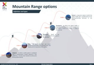
Altiplano Options
Al·ti·pla·no [al-tuh-plah-noh; for 1 also Spanish ahl-tee-plah-naw]
1.A plateau region in South America, situated in the Andes of Argentina, Bolivia and Peru.
2.Financial instrument in which a vanilla option is combined with a compensatory coupon payment if the underlying security never reaches its strike price during a given period.](https://image.slidesharecdn.com/mountain-range-options-141124090640-conversion-gate01/85/Mountain-Range-Options-5-320.jpg)
![Copyright © Arkus Financial Services - 2014
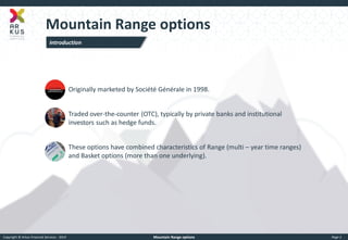
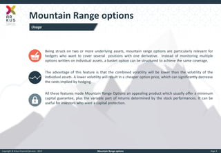
Mountain Range options
Page 8
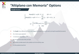
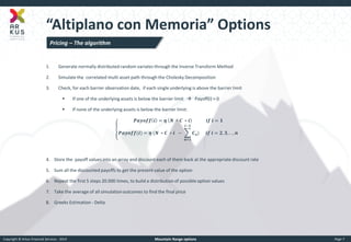
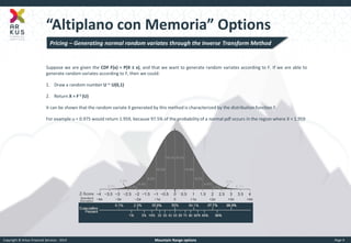
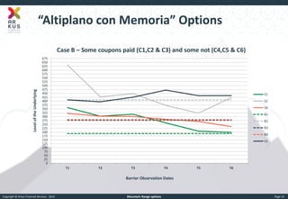
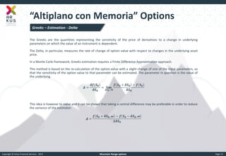
“Altiplano con Memoria” Options
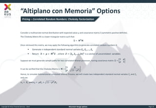
Consider an integral on the unit interval [0,1]:
푰= 품풙풅풙 ퟏ ퟎ
We may think of this integral as the expected value E[g(U)], where U is a uniform random variable on the interval (0,1) and estimate the expected value - a number – by a sample mean (which is a random variable).
The only thing we have to do is generating a sequence Ui of independent random samples from the uniform distribution and then evaluate the sample mean: 푰풎= ퟏ 풎 품(푼풊) 풎 풊=ퟏ
The strong law of large numbers implies that, with probability 1, 풍풊풎 풎 → + ∞ 푰풎=푰
Pricing: the idea behind Monte Carlo Integration](https://image.slidesharecdn.com/mountain-range-options-141124090640-conversion-gate01/85/Mountain-Range-Options-8-320.jpg)


Mountain Range options are basket options that combine characteristics of range options and multi-asset basket options. They are structured on two or more underlying assets and allow hedgers to cover multiple positions with one derivative. Monte Carlo simulation is commonly used to price Mountain Range options since a closed-form solution is not possible due to the complexity of estimating correlations between many underlyings. Greeks such as Delta can also be estimated using finite difference approximations in the Monte Carlo framework.


![Senior Project [Hien Truong, 4204745]](https://cdn.slidesharecdn.com/ss_thumbnails/a82856d9-6fc7-4bef-9d6b-c3ea4bbadfc0-150720053419-lva1-app6892-thumbnail.jpg?width=640&height=640&fit=bounds)