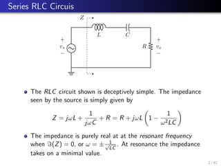
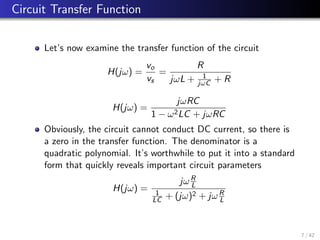
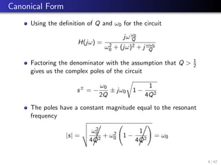
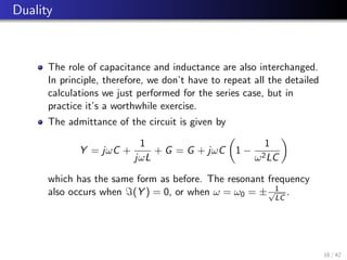
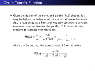
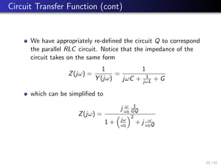
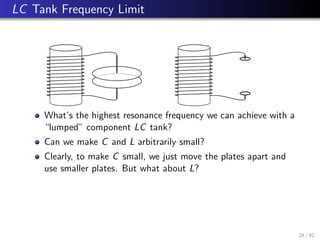
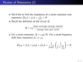
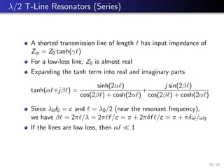
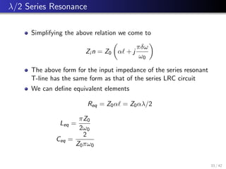
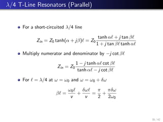
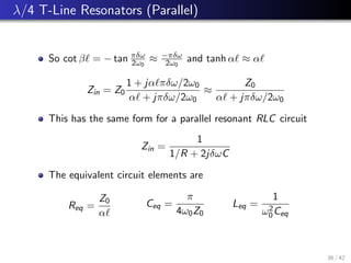
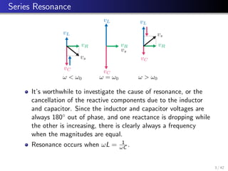
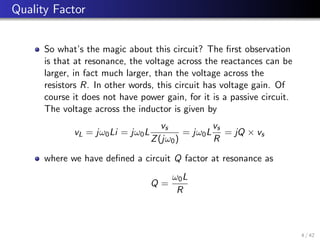
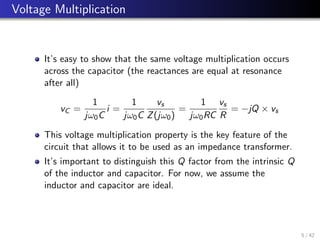
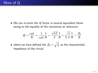
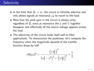
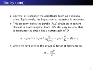
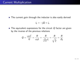
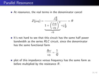
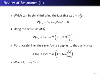
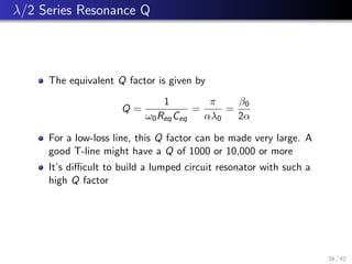
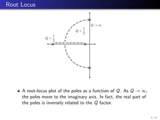
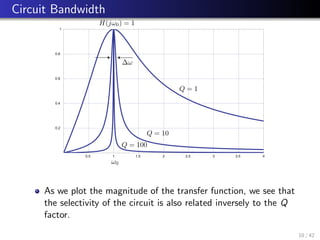
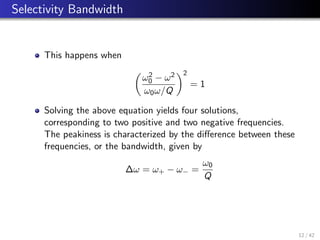
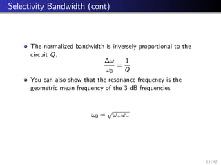
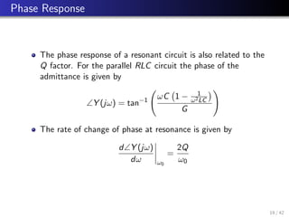
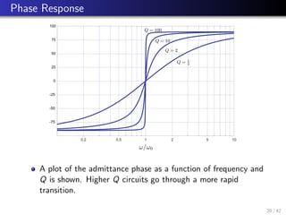
This document summarizes key concepts about RLC circuits: 1. RLC circuits can exhibit resonance where the impedance/admittance is minimized. This occurs at the resonant frequency defined by ω0 = 1/√LC. 2. At resonance, the reactive components (inductance and capacitance) cancel out. The voltage/current is multiplied by the quality factor Q. 3. Higher Q circuits have narrower bandwidth and are more selectively tuned to the resonant frequency. The bandwidth is inversely proportional to Q.

1. Berkeley
Review of Resonance
Prof. Ali M. Niknejad
U.C. Berkeley
Copyright c 2016 by Ali M. Niknejad
February 6, 2016
1 / 42

2. Series RLC Circuis
Z
L
R
C
+
vs
−
+
vo
−
The RLC circuit shown is deceptively simple. The impedance
seen by the source is simply given by
Z = jωL +
1
jωC
+ R = R + jωL
1 −
1
ω2LC
The impedance is purely real at at the resonant frequency
when =(Z) = 0, or ω = ± 1
√
LC
. At resonance the impedance
takes on a minimal value.
2 / 42

3. Series Resonance
vR
vC
vL
vs
ω ω0 ω = ω0
vR
vC
vL
vs
ω ω0
vR
vC
vL
vs
It’s worthwhile to investigate the cause of resonance, or the
cancellation of the reactive components due to the inductor
and capacitor. Since the inductor and capacitor voltages are
always 180◦ out of phase, and one reactance is dropping while
the other is increasing, there is clearly always a frequency
when the magnitudes are equal.
Resonance occurs when ωL = 1
ωC .
3 / 42

4. Quality Factor
So what’s the magic about this circuit? The first observation
is that at resonance, the voltage across the reactances can be
larger, in fact much larger, than the voltage across the
resistors R. In other words, this circuit has voltage gain. Of
course it does not have power gain, for it is a passive circuit.
The voltage across the inductor is given by
vL = jω0Li = jω0L
vs
Z(jω0)
= jω0L
vs
R
= jQ × vs
where we have defined a circuit Q factor at resonance as
Q =
ω0L
R
4 / 42

5. Voltage Multiplication
It’s easy to show that the same voltage multiplication occurs
across the capacitor (the reactances are equal at resonance
after all)
vC =
1
jω0C
i =
1
jω0C
vs
Z(jω0)
=
1
jω0RC
vs
R
= −jQ × vs
This voltage multiplication property is the key feature of the
circuit that allows it to be used as an impedance transformer.
It’s important to distinguish this Q factor from the intrinsic Q
of the inductor and capacitor. For now, we assume the
inductor and capacitor are ideal.
5 / 42

6. More of Q
We can re-write the Q factor in several equivalent forms
owing to the equality of the reactances at resonance
Q =
ω0L
R
=
1
ω0C
1
R
=
√
LC
C
1
R
=
r
L
C
1
R
=
Z0
R
where we have defined the Z0 =
q
L
C as the characteristic
impedance of the circuit.
6 / 42

7. Circuit Transfer Function
Let’s now examine the transfer function of the circuit
H(jω) =
vo
vs
=
R
jωL + 1
jωC + R
H(jω) =
jωRC
1 − ω2LC + jωRC
Obviously, the circuit cannot conduct DC current, so there is
a zero in the transfer function. The denominator is a
quadratic polynomial. It’s worthwhile to put it into a standard
form that quickly reveals important circuit parameters
H(jω) =
jωR
L
1
LC + (jω)2 + jωR
L
7 / 42

8. Canonical Form
Using the definition of Q and ω0 for the circuit
H(jω) =
jωω0
Q
ω2
0 + (jω)2 + j ωω0
Q
Factoring the denominator with the assumption that Q 1
2
gives us the complex poles of the circuit
s±
= −
ω0
2Q
± jω0
r
1 −
1
4Q2
The poles have a constant magnitude equal to the resonant
frequency
|s| =
v
u
u
t ω2
0
4Q2
,
+ ω2
0 1 −
1
4Q2
,!
= ω0
8 / 42

9. Root Locus
Q → ∞
Q
1
2
Q
1
2
!
!
!
!
!
!
!!!!
!
!
!
!
!
!
!!!!
!!!
A root-locus plot of the poles as a function of Q. As Q → ∞,
the poles move to the imaginary axis. In fact, the real part of
the poles is inversely related to the Q factor.
9 / 42

10. Circuit Bandwidth
0.5 1 1.5 2 2.5 3 3.5 4
0.2
0.4
0.6
0.8
1
Q = 1
Q = 10
Q = 100
H(jω0) = 1
∆ω
ω0
As we plot the magnitude of the transfer function, we see that
the selectivity of the circuit is also related inversely to the Q
factor.
10 / 42

11. Selectivity
In the limit that Q → ∞, the circuit is infinitely selective and
only allows signals at resonance ω0 to travel to the load.
Note that the peak gain in the circuit is always unity,
regardless of Q, since at resonance the L and C together
disappear and effectively all the source voltage appears across
the load.
The selectivity of the circuit lends itself well to filter
applications. To characterize the peakiness, let’s compute the
frequency when the magnitude squared of the transfer
function drops by half
|H(jω)|2
=
ωω0
Q
2
ω2
0 − ω2
2
+
ωω0
Q
2
=
1
2
11 / 42

12. Selectivity Bandwidth
This happens when
ω2
0 − ω2
ω0ω/Q
2
= 1
Solving the above equation yields four solutions,
corresponding to two positive and two negative frequencies.
The peakiness is characterized by the difference between these
frequencies, or the bandwidth, given by
∆ω = ω+ − ω− =
ω0
Q
12 / 42

13. Selectivity Bandwidth (cont)
The normalized bandwidth is inversely proportional to the
circuit Q.
∆ω
ω0
=
1
Q
You can also show that the resonance frequency is the
geometric mean frequency of the 3 dB frequencies
ω0 =
√
ω+ω−
13 / 42

14. Parallel RLC Circuits
14 / 42

15. Parallel RLC
Y
L R
C
is
io
The parallel RLC circuit is the dual of the series circuit. By
“dual” we mean that the role of voltage and currents are
interchanged.
Hence the circuit is most naturally probed with a current
source is. In other words, the circuit has current gain as
opposed to voltage gain, and the admittance minimizes at
resonance as opposed to the impedance.
15 / 42

16. Duality
The role of capacitance and inductance are also interchanged.
In principle, therefore, we don’t have to repeat all the detailed
calculations we just performed for the series case, but in
practice it’s a worthwhile exercise.
The admittance of the circuit is given by
Y = jωC +
1
jωL
+ G = G + jωC
1 −
1
ω2LC
which has the same form as before. The resonant frequency
also occurs when =(Y ) = 0, or when ω = ω0 = ± 1
√
LC
.
16 / 42

17. Duality (cont)
Likewise, at resonance the admittance takes on a minimal
value. Equivalently, the impedance at resonance is maximum.
This property makes the parallel RLC circuit an important
element in tuned amplifier loads. It’s also easy to show that
at resonance the circuit has a current gain of Q
iC = jω0Cvo = jω0C
is
Y (jω0)
= jω0C
is
G
= jQ × is
where we have defined the circuit Q factor at resonance by
Q =
ω0C
G
17 / 42

18. Current Multiplication
The current gain through the inductor is also easily derived
iL = −jQ × is
The equivalent expressions for the circuit Q factor are given
by the inverse of the previous relations
Q =
ω0C
G
=
R
ω0L
=
R
1
√
LC
L
=
R
q
L
C
=
R
Z0
18 / 42

19. Phase Response
The phase response of a resonant circuit is also related to the
Q factor. For the parallel RLC circuit the phase of the
admittance is given by
∠Y (jω) = tan−1 ωC 1 − 1
ω2LC
G
!
The rate of change of phase at resonance is given by
d∠Y (jω)
dω ω0
=
2Q
ω0
19 / 42

20. Phase Response
0.2 0.5 1 2 5 10
-75
-50
-25
0
25
50
75
100
ω/ω0
Q = 100
Q = 10
Q = 2
Q = 1
2
A plot of the admittance phase as a function of frequency and
Q is shown. Higher Q circuits go through a more rapid
transition.
20 / 42

21. Circuit Transfer Function
Given the duality of the series and parallel RLC circuits, it’s
easy to deduce the behavior of the circuit. Whereas the series
RLC circuit acted as a filter and was only sensitive to voltages
near resonance ω0, likewise the parallel RLC circuit is only
sensitive to currents near resonance
H(jω) =
io
is
=
voG
voY (jω)
=
G
jωC + 1
jωL + G
which can be put into the same canonical form as before
H(jω) =
jωω0
Q
ω2
0 + (jω)2 + j ωω0
Q
21 / 42

22. Circuit Transfer Function (cont)
We have appropriately re-defined the circuit Q to correspond
the parallel RLC circuit. Notice that the impedance of the
circuit takes on the same form
Z(jω) =
1
Y (jω)
=
1
jωC + 1
jωL + G
which can be simplified to
Z(jω) =
j ω
ω0
1
GQ
1 +
jω
ω0
2
+ j ω
ω0Q
22 / 42

23. Parallel Resonance
At resonance, the real terms in the denominator cancel
Z(jω0) =
j R
Q
1 +
jω0
ω0
2
| {z }
=0
+j 1
Q
= R
It’s not hard to see that this circuit has the same half power
bandwidth as the series RLC circuit, since the denominator
has the same functional form
∆ω
ω0
=
1
Q
plot of this impedance versus frequency has the same form as
before multiplied by the resistance R.
23 / 42

24. LC Tank Frequency Limit
What’s the highest resonance frequency we can achieve with a
“lumped” component LC tank?
Can we make C and L arbitrarily small?
Clearly, to make C small, we just move the plates apart and
use smaller plates. But what about L?
24 / 42

25. Small Capacitor → Bigger Inductor
“inductor”
“inductor”
As shown above, the smallest “inductor” has zero turns, or
it’s just straight wire connected to the capacitor.
Since inductance is defined for a loop, the capacitor is actually
now part of the inductor and defines the inductance of the
circuit.
To make the inductance smaller requires that we increase the
capacitor (bring plates closer).
25 / 42

26. Feynman’s Can
Given a fixed plate spacing and size, we can also be clever and
keep adding inductors in parallel to reduce the inductance.
In the limit, we end up with a “can”!
High frequency resonators are built this way from the outset,
rather than from lumped components.
26 / 42

27. Shorted Line Impedance
.25 .5 .75 1.0 1.25
-7.5
-5
-2.5
0
2. 5
5
7. 5
10
jX(z)
z
λ
Recall the behavior of a shorted line when its length is a
quarter wavelength
Notice that the line is exactly λ/4 at a particular frequency. If
we change the frequency, the line becomes either inductive or
capacitive
Also, if the line has loss, we might expect that the line cannot
be a true open circuit, but a high impedance.
27 / 42

28. Lossy Transmission Line Impedance
Using the same methods to calculate the impedance for the
low-loss line, we arrive at the following line voltage/current
v(z) = v+
e−γz
(1 + ρLe2γz
) = v+
e−γz
(1 + ρL(z))
i(z) =
v+
Z0
e−γz
(1 − ρL(z))
Where ρL(z) is the complex reflection coefficient at position z
and the load reflection coefficient is unaltered from before
The input impedance is therefore
Zin(z) = Z0
e−γz + ρLeγz
e−γz − ρLeγz
28 / 42

29. Lossy T-Line Impedance (cont)
Substituting the value of ρL we arrive at a similar equation
(now a hyperbolic tangent)
Zin(−`) = Z0
ZL + Z0 tanh(γ`)
Z0 + ZL tanh(γ`)
For a short line, if γδ` 1, we may safely assume that
Zin(−δ`) = Z0 tanh(γδ`) ≈ Z0γδ`
Recall that Z0γ =
p
Z0/Y 0
√
Z0Y 0
As expected, input impedance is therefore the series
impedance of the line (where R = R0δ` and L = L0δ`)
Zin(−δ`) = Z0
δ` = R + jωL
29 / 42

30. Review of Resonance (I)
We’d like to find the impedance of a series resonator near
resonance Z(ω) = jωL + 1
jωC + R
Recall the definition of the circuit Q
Q = ω0
time average energy stored
energy lost per cycle
For a series resonator, Q = ω0L/R. For a small frequency
shift from resonance δω ω0
Z(ω0 + δω) = jω0L + jδωL +
1
jω0C
1
1 + δω
ω0
!
+ R
30 / 42

31. Review of Resonance (II)
Which can be simplified using the fact that ω0L = 1
ω0C
Z(ω0 + δω) = j2δωL + R
Using the definition of Q
Z(ω0 + δω) = R
1 + j2Q
δω
ω0
For a parallel line, the same formula applies to the admittance
Y (ω0 + δω) = G
1 + j2Q
δω
ω0
Where Q = ω0C/G
31 / 42

32. λ/2 T-Line Resonators (Series)
A shorted transmission line of length ` has input impedance of
Zin = Z0 tanh(γ`)
For a low-loss line, Z0 is almost real
Expanding the tanh term into real and imaginary parts
tanh(α`+jβ`) =
sinh(2α`)
cos(2β`) + cosh(2α`)
+
j sin(2β`)
cos(2β`) + cosh(2α`)
Since λ0f0 = c and ` = λ0/2 (near the resonant frequency),
we have β` = 2π`/λ = 2π`f /c = π + 2πδf `/c = π + πδω/ω0
If the lines are low loss, then α` 1
32 / 42

33. λ/2 Series Resonance
Simplifying the above relation we come to
Zi n = Z0
α` + j
πδω
ω0
The above form for the input impedance of the series resonant
T-line has the same form as that of the series LRC circuit
We can define equivalent elements
Req = Z0α` = Z0αλ/2
Leq =
πZ0
2ω0
Ceq =
2
Z0πω0
33 / 42

34. λ/2 Series Resonance Q
The equivalent Q factor is given by
Q =
1
ω0ReqCeq
=
π
αλ0
=
β0
2α
For a low-loss line, this Q factor can be made very large. A
good T-line might have a Q of 1000 or 10,000 or more
It’s difficult to build a lumped circuit resonator with such a
high Q factor
34 / 42

35. λ/4 T-Line Resonators (Parallel)
For a short-circuited λ/4 line
Zin = Z0 tanh(α + jβ)` = Z0
tanh α` + j tan β`
1 + j tan β` tanh α`
Multiply numerator and denominator by −j cot β`
Zin = Z0
1 − j tanh α` cot β`
tanh α` − j cot β`
For ` = λ/4 at ω = ω0 and ω = ω0 + δω
β` =
ω0`
v
+
δω`
v
=
π
2
+
πδω
2ω0
35 / 42

36. λ/4 T-Line Resonators (Parallel)
So cot β` = − tan πδω
2ω0
≈ −πδω
2ω0
and tanh α` ≈ α`
Zin = Z0
1 + jα`πδω/2ω0
α` + jπδω/2ω0
≈
Z0
α` + jπδω/2ω0
This has the same form for a parallel resonant RLC circuit
Zin =
1
1/R + 2jδωC
The equivalent circuit elements are
Req =
Z0
α`
Ceq =
π
4ω0Z0
Leq =
1
ω2
0Ceq
36 / 42

37. λ/4 T-Line Resonators Q Factor
The quality factor is thus
Q = ω0RC =
π
4α`
=
β
2α
37 / 42

38. Crystal Resonator
C0
L1 C1 R1
R2
R3
L2 C2
L3 C3
t
quartz
Quartz crystal is a piezoelectric material. An electric field
causes a mechanical displacement and vice versa. Thus it is a
electromechanical transducer.
The equivalent circuit contains series LCR circuits that
represent resonant modes of the XTAL. The capacitor C0 is a
physical capacitor that results from the parallel plate
capacitance due to the leads.
38 / 42

39. Fundamental Resonant Mode
Acoustic waves through the crystal have phase velocity
v = 3 × 103 m/s. For a thickness t = 1 mm, the delay time
through the XTAL is given by
τ = t/v = (10−3 m)/(3 × 103 m/s) = 1/3 µs.
This corresponds to a fundamental resonant frequency
f0 = 1/τ = v/t = 3 MHz = 1
2π
√
L1C1
.
The quality factor is extremely high, with Q ∼ 3 × 106 (in
vacuum) and about Q = 1 × 106 (air). This is much higher
than can be acheived with electrical circuit elements
(inductors, capacitors, transmission lines, etc). This high Q
factor leads to good frequency stability (low phase noise).
39 / 42

40. MEMS Resonators
The highest frequency, though, is limited by the thickness of
the material. For t ≈ 15 µm, the frequency is about 200 MHz.
MEMS resonators have been demonstrated up to ∼ GHz
frequencies. MEMS resonators are an active research area.
Integrated MEMS resonators are fabricated from polysilicon
beams (forks), disks, and other mechanical structures. These
resonators are electrostatically induced structures.
40 / 42

41. Example XTAL
C0
L1
C1
R1
Some typical numbers for a
fundamental mode resonator are
C0 = 3 pF, L1 = 0.25 H, C1 = 40 fF,
R1 = 50 Ω, and f0 = 1.6 MHz. Note
that the values of L1 and C1 are
modeling parameters and not physical
inductance/capacitance. The value of
L is large in order to reflect the high
quality factor.
The quality factor is given by
Q =
ωL1
R1
= 50 × 103
=
1
ωR1C1
41 / 42

42. Series and Parallel Mode
C0
L1 C1 R1
C0
L1 R1
low resistance high resistance
Due to the external physical capacitor, there are two resonant
modes between a series branch and the capacitor. In the
series mode ωs, the LCR is a low impedance (“short”). But
beyond this frequency, the LCR is an equivalent inductor that
resonates with the external capacitance to produce a parallel
resonant circuit at frequency ωp ωs.
42 / 42