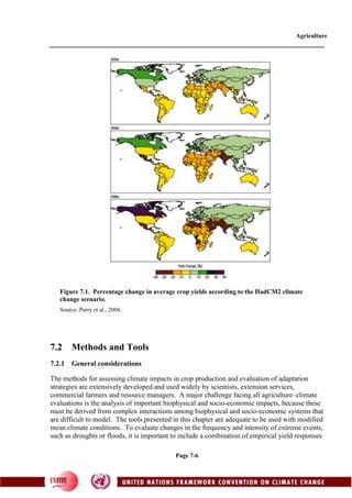
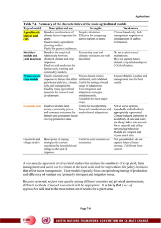
Page 7-1
https://www.youtube.com/watch?v=kFpAavw0lMs
7. Agriculture
7.1 Overview
7.1.1 Context of National Communications
Sustainable development includes social, economic and environmental dimensions. Climate
change modifies all these dimensions and therefore alters the potential development pathways.
In particular, the effects of climate change on agriculture will determine the future of food
security and ultimately influence the inequitable North–South divide.
According to the IPCC TAR (McCarthy et al., 2001), climate change is already happening and
will continue to happen even if global GHG emissions are curtailed. Many studies document
the implications of climate change for agriculture and pose a reasonable concern that climate
change is a threat to sustainable development, especially in countries not included in Annex I to
the Convention. Identifying which regions and populations are at greatest risk from climate
change (i.e., are most vulnerable) can help in setting priorities for adaptation. This chapter
focuses on the methods for making these assessments, and includes examples of applications in
developing countries and an overview of existing knowledge on the subject. The merits of each
approach vary according to the level of impact being studied, and approaches may frequently be
mutually supportive. For example, simple agroclimatic indices often provide the necessary
information on how crops respond to varying rainfall and temperature in wide geographical
areas; crop-specific models are used to test alternative management that can in turn be used as a
component of an economic model that analyses regional vulnerability or national adaptation
strategies. Therefore, a mix of approaches is often most productive.
7.1.2 Effects of current climate variability
Climate is an essential component of the natural capital. In many regions of the world, such as
Africa, Southern and Central America, and South and South-East Asia, climates are extremely
variable from year to year, and recurrent drought and flood problems often affect entire
countries over multi-year periods. These often result in serious social problems. For example,
the persistent drying trend in parts of Africa over the past decades has affected food production,
including freshwater fisheries, industrial and domestic water supplies, and hydropower
generation (Benson and Clay, 1998, 2000).
Agriculture is strongly dependent on water resources and climatic conditions, particularly in the
regions of the world that are particularly sensitive to climatic hazards, such as Africa, South and
Central America, and Asia. Some countries in these regions, where economic and social
situations are often unstable, are extremely vulnerable to changes in environmental factors. It is
especially the case in countries where technological buffering to droughts and floods is less
advanced, and where the main physical factors affecting production (soils, terrain and climate)
are less suited to farming. Crop production is consequently extremely sensitive to large year-
Agriculture
Page 7-2
to-year weather fluctuations. Crop diseases or pest infestations are also weather dependent and
tend to cause more damage in countries with lower technological levels.
7.1.3 Drivers of agricultural response to climate change
Estimation of future agricultural responses to climate change is usually based on scenarios. It is
crucial to understand that there is large uncertainty in the climate scenarios. The scenarios are
essential for evaluating possible future conditions, but they do not necessarily describe the
conditions that will actually occur. Nevertheless, conditions similar to the scenarios are
possible, and as such they should be used to explore possible adaptive measures.
Agriculture is a complex sector involving different driving parameters (environmental,
economic and social). It is now well recognized that crop production is very sensitive to
climate change (McCarthy et al., 2001), with different effects according to region. The IPCC
analysis of climate change impacts (TAR) estimates a general reduction of potential crop yields
and a decrease in water availability for agriculture and populations in many parts of the
developing world (Table 7.1).
The main drivers of agricultural responses to climate change are biophysical effects (Table 7.2)
and socio-economic factors (Table 7.3). Crop production is affected biophysically by changing
meteorological variables, including rising temperatures, changing precipitation regimes and
increasing levels of atmospheric carbon dioxide. Biophysical effects of climate change on
agricultural production depend on the region and the agricultural system, and the effects vary
through time.
Socio-economic factors influence responses to changes in crop productivity, with price changes
and shifts in comparative advantage. The final response depends on the adaptation strategies in
each region and agricultural system. The combination of biophysical and socio-economic
effects can result in:
 Changes in the mix of crops grown, and hence in the type of farming and rural land use
 Changes in production, farm income, and rural employment
 Changes in rural income, contribution to national GDP, and agricultural export earnings.
Table 7.1. Climate change and related factors relevant to agricultural production and
food security
Climate factor Direction of change
Consequences and factors that interact with
agricultural production and food security
Sea level rise Increase Sea level intrusion in coastal (agricultural) areas and
salinization of water supply
Precipitation
intensity/run-off
Intensified hydrological cycle, so
generally increases, but with
regional variations
Changed patterns of erosion and accretion; changed
storm impacts; changed occurrence of storm flooding
and storm damage, water logging, increase in pests
Heat stress Increases in heat waves Damage to grain formation, increase in some pests
Drought Poorly known, but significant
increased temporal and spatial
variability expected
Crop failure, yield decrease; competition for water
Atmospheric CO2 Increase Increased crop productivity but also increased weed
productivity and therefore competition with crops
Agriculture
Page 7-3
Source: Data and information from Parry et al. (1998a, 2004), McCarthy et al. (2001).
Agriculture
Page 7-4
Table 7.2. Characterization of agronomic impacts, adaptive capacity and sector outcomes
Biophysical
impact
Uncertainty
level
Expected intensity
of negative effects
Adaptive
capacity
Socio-economic and other
secondary impacts
Changes in crop
growth conditions
Medium High for some
crops and regions
Moderate
to high
Changes in optimal farming systems;
relocation of farm processing industry;
increased economic risk; loss of rural
income; pollution due to nutrient
leaching; biodiversity decrease
Changes in
optimal conditions
for livestock
production
High Medium High for
intensive
production
systems
Changes in optimal farming systems;
loss of rural income
Changes in
precipitation and
the availability of
water resources
Medium
to low
High for
developing
countries
Moderate Increased demand for irrigation;
decreased yield of crops; increased risk
of soil salinization; increased water
shortage; loss of rural income
Changes in
agricultural pests
High to
very high
Medium Moderate
to high
Pollution due to increased use of
pesticides; decreased yield and quality of
crops; increased economic risk; loss of
rural income
Changes in soil
fertility and
erosion
Medium High for
developing
countries
Moderate Pollution by nutrient leaching;
biodiversity decrease; decreased yield of
crops; land abandonment; increased risk
of desertification; loss of rural income
Table 7.3. Characterization of aggregated farming system impacts, adaptive capacity and
sector outcomes
Socio-economic
impact
Uncertainty
level
Expected intensity
of negative effects
Autonomous
adaptation (private
coping capacity) Other impacts
Changes in
optimal farming
systems
High High for areas where
current optimal
farming systems are
extensive
Moderate Changes in crop and livestock
production activities; relocation of
farm processing industry; loss of
rural income; pollution due to
nutrient leaching; biodiversity
decrease
Relocation of
farm processing
industry
High High for some food
industries requiring
large infrastructure
or local labour
Moderate Loss of rural income; loss of
cultural heritage
Increased
(economic) risk
Medium High for crops
cultivated near their
climatic limits
Low Loss of rural income
Loss of rural
income and
cultural heritage
High (Not characterized) Moderate Land abandonment; increased risk
of desertification; welfare decrease
in rural societies; migration to
urban areas; biodiversity decrease
Agriculture
Page 7-5
7.1.4 Previous studies
Several hundred studies on climate change as it relates to agriculture have been completed.
They provide a first indication of the impact types to expect, and thus the most effective
analysis methods to implement. Potential impacts on world food supply have been estimated
for several climate change and socio-economic scenarios (Figure 7.1). Some regions may enjoy
improved agricultural production, whereas others will suffer from yield losses, and so a
reorganization of agricultural production areas may be required. In any given region, crops are
expected to be affected differently, leading to the need for adaptation in related support
industries and markets, farm-level strategies and rural development schemes.
Although Figure 7.1 shows that global production appears stable (Parry et al., 2004 provide
additional quantitative data), regional differences in crop production are likely to grow through
time, leading to a significant polarization of effects with substantial increases in prices and risk
of hunger in the poorer nations. The most serious effects are at the margins – in vulnerable
regions and among vulnerable groups. Individuals particularly vulnerable to environmental
change are those with relatively high exposures to changes, high sensitivity to changes, low
coping and adaptive capacities, and low resilience and recovery potential. Adaptation is
necessary, but adaptation has limits (technological, biotechnological, political, cultural).
Agriculture
Page 7-6
7.2 Methods and Tools
7.2.1 General considerations
The methods for assessing climate impacts in crop production and evaluation of adaptation
strategies are extensively developed and used widely by scientists, extension services,
commercial farmers and resource managers. A major challenge facing all agriculture–climate
evaluations is the analysis of important biophysical and socio-economic impacts, because these
must be derived from complex interactions among biophysical and socio-economic systems that
are difficult to model. The tools presented in this chapter are adequate to be used with modified
mean climate conditions. To evaluate changes in the frequency and intensity of extreme events,
such as droughts or floods, it is important to include a combination of empirical yield responses
Figure 7.1. Percentage change in average crop yields according to the HadCM2 climate
change scenario.
Source: Parry et al., 2004.
Agriculture
Page 7-7
based on statistical data and modelling approaches. In all cases, the challenge in interpreting
the results originates in the use of uncertain climate change scenarios.
A number of approaches to the assessment of the impacts of climate change on agriculture have
been developed from the many studies conducted to date. Approaches used to assess
biophysical impacts include:
 Agroclimatic indices and GIS
 Statistical models and yield functions
 Process-based models.
In addition, different tools can be used to examine the socio-economic impacts of climate
change. A relatively simple economic forecasting tool, such as that developed by the United
States Country Studies Program (Benioff et al., 1996), is often useful. More complex
approaches, such as economic regression models, microeconomic and macroeconomic models,
farm models, and household and village models, can also be used.
Each of these methods yields information on different types of impacts (Table 7.4). For
example, simple agroclimatic indices can be used to analyse large-area shifts of cropping zones,
whereas process-based crop growth models should be used to analyse changes in crop yields.
Effects on income, livelihoods and employment are assessed using economic and social forms
of analysis.
In addition, studies can be undertaken using a regional approach or a site-specific approach. In
a regional approach, several existing simple tools can be applied and tested under a range of
conditions in a given region and the results visualized on maps. This simple regional approach
is essential for integrating climate change, crop production, water demand indices and socio-
economic indices on a regional scale, thus providing a first-order evaluating tool to analyse
possible adaptation strategies.
Agriculture
Page 7-8
Table 7.4. Summary of the characteristics of the main agricultural models
Type of model Description and use Strengths Weaknesses
Agroclimatic
indices and
GIS
Based on combinations of
climate factors important for
crops.
Used in many agricultural
planning studies.
Useful for general audiences.
Simple calculation.
Effective for comparing
across regions or crops.
Climate based only, lack
management responses or
consideration of carbon
fertilization.
Statistical
models and
yield functions
Based on the empirical
relationship between
observed climate and crop
responses.
Used in yield prediction for
famine early warning and
commodity markets.
Present-day crop and
climatic variations are well
described.
Do not explain causal
mechanisms.
May not capture future
climate–crop relationships or
CO2 fertilization.
Process-based
crop models
Used to calculate crop
responses to factors that affect
growth and yield (i.e., climate,
soils, and management).
Used by many agricultural
scientists for research and
development.
Process based, widely
calibrated, and validated.
Useful for testing a broad
range of adaptations.
Test mitigation and
adaptation strategies
simultaneously.
Available for most major
crops.
Require detailed weather and
management data for best
results.
Economic tools Used to calculate land
values, commodity prices,
and economic outcomes for
farmers and consumers based
on crop production data.
Useful for incorporating
financial considerations and
market-based adaptations.
Not all social systems,
households and individuals
appropriately represented.
Climate-induced alterations in
availability of land and water
not always taken into account.
Focus on profit and utility-
maximizing behaviour.
Models are complex and
require much data.
Household and
village models
Description of coping
strategies for current
conditions by household and
village as the unit of
response.
Useful in semi commercial
economies.
Not generalizable; do not
capture future climate
stresses, if different from
current.
A site-specific approach involves local studies that analyse the sensitivity of crop yield, farm
management and water use to climate at the local scale and the implications for policy decisions
that affect water management. Crop models typically focus on optimizing timing of production
and efficiency of nutrient use (primarily nitrogen) and irrigation water.
Because economic sectors vary greatly among different countries and physical environments,
different methods of impact assessment will be appropriate. It is likely that a mix of
approaches will lead to the most robust set of results for a given area.
Agriculture
Page 7-9
7.2.2 Limitations and sources of uncertainty
Climate change scenarios. Climate change scenarios are derived from GCMs driven by
changes in the atmospheric composition of GHG, derived from different storylines in socio-
economic scenarios (SRES, see below). A main challenge is, how to interpret the results
derived from the climate scenarios. In all regions, uncertainties with respect to the magnitude
of the expected changes result in uncertainties in the agricultural evaluations. For example, in
some regions projections of rainfall, a key variable for crop production, may be positive or
negative depending on the climate scenario used. The uncertainty derived from the climate
model is related to the limitation of current models to represent all atmospheric processes and
interactions of the climate system. The limitations associated with projecting socio-economic
development pathways represent an additional source of uncertainty.
Climate variability. Regional climates naturally fluctuate about the long-term mean. For
example, rainfall variability occurs with regard to timing and quantity, affecting agriculture
each year. It is clear that changes have occurred in the past and will continue to occur, and
climate change modifies these variability patterns, for example, resulting in more droughts and
floods. Nevertheless, there are many uncertainties, especially about rainfall scenarios for the
future.
Agricultural models. Agricultural models contain many simple, empirically derived
relationships that do not completely represent actual plant processes. When models are
adequately tested against observed data (calibration and validation process), the results
represent agricultural output under current climate conditions. Nevertheless, the simplifications
of the crop models are a source of uncertainty of the results. For example, agricultural models
in general assume that weeds, diseases and insect pests are controlled; that there are no problem
soil conditions, such as high salinity or acidity; and that there are no catastrophic weather
events, such as heavy storms. The agricultural models simulate the current range of agricultural
technologies available around the world; they do not include potential improvements in such
technology, but can be used to test the effects of some potential improvements, such as
improved varieties and irrigation schedules. A range of agricultural models is used widely by
scientists, technical extension services, commercial farmers and resource managers to evaluate
agricultural alternatives in a given location under different conditions (i.e., drought years,
changes in policy regarding application of agrochemicals, changes in water input, among other
conditions).
Effects of CO2 on crops. CO2 is a component of plant photosynthesis and therefore influences
biomass production. It also regulates the opening of plant stomata and therefore affects plant
transpiration. As a result, in theory, plants growing in increased CO2 conditions will produce
more biomass and will consume less water. Experiments in greenhouses confirm this;
nevertheless because of the multiple interactions of physiological processes, actual changes are
smaller than the theoretical ones. In field conditions, the changes are even smaller. Most of the
crop models used for climate change evaluations include an option to simulate the effects of
CO2 increase on crop yield and water use (see Rosenzweig and Iglesias, 1998). It is difficult to
validate the crop model results because there are only a very limited number of these
experiments worldwide, raising uncertainty about the simulated results.
Issues of scale. Scaling up the vulnerability and adaptation results to a regional level is, as in
most scaling exercises, not an easy task. Ideally, one might use information from farms that are
Agriculture
Page 7-10
representative of agriculture in the region, and the degree of their representativeness would
need to be established. More frequently, regional assessments have relied on the input provided
by regional planners and economists as to regional-scale effects, based on local data supplied to
them and discussed by a full range of stakeholders.
Socio-economic projections. The limitations of projecting socio-economic changes affect not
only the SRES scenarios but also the potential adaptive capacity of the system. For example,
uncertainty about the population changes (density, distribution, migration), GDP, and
technology determines and limits the potential adaptation strategies that can be employed.
7.2.3 Combining climate change scenarios with agricultural tools and models
Given the uncertainties of the scenarios (magnitude of change and sometimes direction of
change), a good approach is to use several possible scenarios as inputs for the agricultural
models. In addition, using sensitivity scenarios combined with agricultural models (for
example, changes in temperature up to +3o
C and changes in precipitation from –30% to +30%)
provides an idea of the tolerable thresholds of change for a particular system.
One method shown to be effective for generating climate change scenarios is to study the
changes in the last few decades and then project those changes into the near future. For
example, divide the long-term climate database of one region (or sites) and divide them into
two periods: for example 1930–1960 and 1970–2000. Then study the statistical properties of
each one of those two datasets (means, but also frequency, of dry spells, of storms, probability
of subsequent days with rainfall, etc.). This can be done with “weather generators”. The last
step is to continue (project) the trend observed in all these statistical parameters and create a
synthetic scenario for the near future (e.g., 10–20 years). This method has the advantage that it
is based in observed changes. Of course the projections may be as bad as (or worse than) the
results using the conventional method of GCMs.
Finally, an interesting approach is to use a scenario that occurs within the natural climate
variability of the region, such as a drought scenario. It is essential that the agricultural
evaluations include and test more than one possible scenario and analyse the sensitivity of the
response in the context of the current trends of climate. The use of more than one scenario and
approach results in a span of outcomes, which gives a pertinent notion of uncertainty.
7.2.4 Agroclimatic indices and GIS
Simple agroclimatic indices combined with GIS have been used to provide an initial evaluation
of both global agricultural climate change impacts and shifts in agriculturally suitable areas in
particular regions. The agroclimatic indices are based on simple relationships of crop
suitability or potential to climate (e.g., identifying the temperature thresholds of a given crop or
using accumulated temperature over the growing season to predict crop yields; e.g., Holden,
2001). This type of empirically derived coefficient is especially useful for broad-scale mapping
of areas of potential impact.
When combined with a spatially comprehensive database of climate, crops and GIS, simple
agroclimatic indices are an inexpensive and rapid way of mapping altered crop potential for
quite large areas. Applying agroclimatic indices in Africa (Badini et al., 1997) has provided an
Agriculture
Page 7-11
understanding of the relationships between the weather, soils and agricultural production
systems and the complexities associated with their variability. Carter and Saarikko (1996)
describe basic methods for agroclimatic spatial analysis.
7.2.5 Statistical models and yield functions
Complex multivariate models attempt to provide a statistical explanation of observed
phenomena by accounting for the most important factors (e.g., predicting crop yields on the
basis of temperature, rainfall, sowing date and fertilizer application). A possible weakness in
their use for examining the impacts of future climate change, however, is their limited ability to
predict effects of climatic events that lie outside the range of present-day variability. Their use
has also been criticized because they are based on statistical relationships between factors rather
than on an understanding of the important causal mechanisms.
Multiple regression models have been developed to represent process-based yield responses to
these environmental and management variables. Yield functions have been used to evaluate the
sensitivity and adaptation to climate, e.g., in China (Rosenzweig et al., 1999) and globally (Parry et
al., 2004).
7.2.6 Process-based crop models
Process-based models use simplified functions to express the interactions between crop growth and
the major environmental factors that affect crops (i.e., climate, soils and management), and many
have been used in climate impact assessments. Most were developed as tools in agricultural
management, particularly for providing information on the optimal amounts of input (such as
fertilizers, pesticides and irrigation) and their optimal timing. Dynamic crop models are now
available for most of the major crops. In each case, the aim is to predict the response of a given
crop to specific climate, soil and management factors governing production.
The ICASA/IBSNAT dynamic crop growth models (International Consortium for Application of
Systems Approaches to Agriculture – International Benchmark Sites Network for Agrotechnology
Transfer) are structured as a decision support system to facilitate simulations of crop responses to
management (DSSAT). The ICASA/IBSNAT models have been used widely for evaluating
climate impacts in agriculture at different levels ranging from individual sites to wide geographic
areas (see Rosenzweig and Iglesias, 1994, 1998, for a full description of the method). This type of
model structure is particularly useful in evaluating the adaptation of agricultural management to
climate change. The DSSAT software includes all ICASA/IBSNAT models with an interface that
allows output analysis.
The WOFOST model suite is generic and includes model parameters for certain crops (Supit et al.,
1994; Boogaard et al., 1998). There are several versions of the models, which are under
continuous development at the University of Wageningen.
The EPIC model (Erosion Productivity Impact Calculator; Sharpley and Williams, 1990)
incorporates simplified crop growth functions that respond to climate, environment and
management; it has been used in some climate impact assessments.
Agriculture
Page 7-12
CROPWAT is an empirical irrigation management model developed by the FAO to calculate
regional crop water and irrigation requirements from climatic and crop data (CROPWAT, 1995,
2004). Net irrigation demand (balance between the crop evapotranspiration and the water
available for the crop) can be calculated for more than 1,000 sites around the world included in
the FAOClim database (FAO, 2004). The model can be adjusted to include irrigation efficiency
for each region.
Table 7.5 summarizes the main crop models that have been used for evaluating impacts and
adaptation to climate change. Rosenzweig and Iglesias (1998) provide more complete guidelines
for using crop models in adaptation studies.
Table 7.5. Crop models
Crop Model
Crop specific ICASA/IBSANT crop-specific models included in the DSSAT software
(including all CERES and GRO models listed under each crop)
Generic WOFOST provides a family of generic models with specific parameters
for maize, wheat, sugar beet and more
General model EPIC
Water irrigation
requirements for all crops
CROPWAT
Alfalfa ALSIM, ALFALFA
Barley CERES-Barley
Cotton GOSSYM, COTCROP, COTTAM
Dry beans BEANGRO
Maize CERES-Maize, CORNF, SIMAIZ, CORNMOD, VT-Maize, GAPS,
CUPID
Peanuts PNUTGRO
Pearl millet CERES-Millet, RESCAP
Potatoes SUBSTOR
Rice CERES-Rice, RICEMOD
Sorghum CERES-Sorghum, SORGF, SORKAM, RESCAP
Soybeans SOYGRO, GLYCIM, REALSOY, SOYMOD
Sugarcane CANEMOD
Wheat CERES-Wheat, TAMW, SIMTAG, AFRCWHEAT, NWHEAT,
SIRIUS, SOILN-Wheat
Agriculture
Page 7-13
Box 7.1 provides more information on DSSAT as an example of a crop-specific family of
models, and Box 7.2 provides more information on WOFOST as an example of a generic
model.
Box 7.1. Description of the DSSAT crop models.
Description: The DSSAT models use simplified functions to predict the growth of crops as influenced by the
major factors that affect yields, i.e., genetics, climate (daily solar radiation, maximum and minimum
temperatures, and precipitation), soils, and management. Models are available for many crops (see Table
7.5); these have been validated over a wide range of environments and are not specific to any particular
location or soil type. Modelled processes include phenological development, growth of vegetative and
reproductive plant parts, extension growth of leaves and stems, senescence of leaves, biomass production and
partitioning among plant parts, and root system dynamics. The models include subroutines to simulate the
soil and crop water balance and the nitrogen balance.
Variables: The primary variable influencing each phase of plant development is temperature. Potential dry
matter production is a function of intercepted radiation; the interception by the canopy is determined by leaf
area. The dry matter allocation to different parts of the plant (grain, leaves, stem, roots, etc.) is determined by
phenological stage and degree of water stress. Final grain yield is the product of plant population, kernels per
plant, and kernel weight. To account for the effect of elevated carbon dioxide on stomatal closure and
increased leaf area index, a ratio of transpiration under elevated CO2 conditions to that under ambient
conditions is added.
Inputs
Type of data Requirements Source of data
Current climate Daily maximum and minimum
temperatures and solar radiation
for at least a 20-year period
National meteorological or research
institutions. Daily data may be simulated
from monthly averages when not
available
Modified climate (climate
change scenarios)
Modified daily maximum and
minimum temperatures,
precipitation, and solar radiation
for a period of the same length as
the current climate
National meteorological or research
institutions
Crop management Crop variety, sowing date and
density, fertilizer and irrigation
inputs (dates and amounts)
Agricultural research institutions
Soils Soil albedo and drainage, and a
description of the different layers
of the soil profile (texture, water
holding capacity, organic matter
and nitrogen)
Agricultural or hydrological research
institutions
Economics (optional) Cost of labour and price of unit
production
Agricultural statistics
Outputs: Variables in the summary output file are the main phenological events, yield, and yield components.
For more information: Rosenzweig and Iglesias, 1994, 1998.
Agriculture
Page 7-14
Box 7.2. Description of WOFOST.
Description: WOFOST originated in the framework of an interdisciplinary study on potential world food
production by the Centre for World Food Studies (CWFS) in cooperation with the Wageningen Agricultural
University. Related models are the successive SUCROS models (Simple and Universal CROP Growth
Simulator), ARID CROP, Spring wheat, MACROS, and ORYZA1. WOFOST version 6.0 is a mechanistic
model that explains crop growth on the basis of photosynthesis and respiration, and how these processes are
affected by environmental conditions. The crop growth model is generic and includes model parameters for
wheat, grain maize, barley, rice, sugar beet, potato, field bean, soybean, oilseed rape and sunflower.
Inputs: Meteorological data (rain, temperature, wind speed, global radiation, air humidity) are needed as
input. Other input data include volumetric soil moisture content at various suction levels and other data on
saturated and unsaturated water flow. Also, data on site-specific soil and crop management are required. The
time step for simulation is one day. WOFOST 6.0 includes an option to use average (monthly) weather data.
Daily rainfall data are generated using a built-in mathematical generator.
Outputs: The model describes crop growth as biomass accumulation in combination with phenological
development.
For more information: Supit et al., 1994; Boogaard et al., 1998.
7.2.7 Calibration and validation of the crop models
Crop models are tools for assessing vulnerability and adaptation to climate change: stakeholder;
participation is essential. A mandatory first step is that technical stakeholders assemble field
agricultural data for calibration and validation of the crop models. Then regional stakeholders
evaluate the representativeness of the agricultural model results for spatial upscaling of the
model results.
In all agricultural models, the procedure involves adjusting coefficients that describe crop
characteristics and response to environmental conditions. Table 7.6 summarizes the steps
involved in calibrating and validating the agricultural models, with specific references relevant
to the DSSAT models as an example. In the DSSAT models, the coefficients that need to be
adjusted are included in a file of “genetic coefficients” that conceptually represent each crop
variety. A file with genetic coefficients for each crop for the most commonly used varieties,
adjusted based on numerous previous and referenced field experiments, is included in the
software. These coefficients are only a starting point and should be further adjusted in the
calibration process to represent crop growth and development of the selected variety under the
climate and management conditions of the particular area. The few genetic coefficients that
describe each variety attempt to represent only the phenology or time of developmental phases
(e.g., juvenile stage, flowering, physiological maturity) and the accumulation of dry mater in
the different organs (e.g., roots, vegetative parts and grain). The few coefficients do not attempt
to represent the very large number of characteristics of each crop variety, such as response to
pests and diseases.
Agriculture
Page 7-15
Table 7.6. Summary of steps for calibrating and validating crop models
Step Concept/procedure Example
1. Calibrate crop
phenology
The crop developmental stage
determines how the biomass is
accumulated and to which organ of
the plant growth is directed.
Adjust the simulated dates on
flowering and physiological maturity
to field data.
In the CERES-Maize model this is described by
the coefficients P1 (thermal time from seedling
emergence to the end of the juvenile phase); P2
(extent to which development is delayed for each
hour increase in photoperiod); and P5 (thermal
time from silking to physiological maturity).
By adjusting these coefficients the development
of the crop can be adjusted to the development in
the field.
2. Calibrate
grain production
The adequate rate and quantity of
biomass accumulation determines
final crop productivity.
Adjust the simulated grain yield to
field data.
In the CERES-Maize model this is described by
the coefficients G2 (maximum possible number
of kernels per plant) and G3 (kernel filling rate
during the linear grain filling stage and under
optimum conditions).
3. Validate the
calibrated model
Ensure that the adjustment of crop
model results with one experimental
field dataset to represent a wider
agricultural area.
Test if the simulated crop flowering
and maturity dates and grain yield
represent farmers’ results.
Well-calibrated models should always simulate
correctly the dates of crop maturity. Simulated
yields may be higher than the ones observed on
farms, but they should represent the geographic
variation of farm yields arising from different
soils or management conditions.
7.2.8 Economic tools
Economic models are designed to estimate the potential impacts of climate change on production,
consumption, income, GDP, employment and farm value. These may be only partial indicators of
social welfare, however. Not all social systems, households, and individuals (for example,
smallholder farmers) may be appropriately represented in models that are based on producer and
consumer theory. Many of the economic models used in impact analyses to date do not account
for the climate-induced alterations in the availability of land and water for irrigation, although such
important considerations can be included. Studies and models based on market-oriented
economies assume profit and utility maximizing behaviour.
Several types of economic approaches have been used for agricultural impact assessment. The
most useful of these are simple economic forecasting approaches (e.g., Benioff et al., 1996), which
are forecasts based on a structured framework of available economic (production, consumption
and governing policies) and agricultural (production techniques and alternative crops) information.
These are generally simple techniques that can be used in most climate impact studies.
The following approaches can also be used, although they are relatively complicated and may be
difficult, time consuming or expensive to apply.
Economic cross-sectional models. One form of economic analysis is the use of spatial analogues,
that is, cropping patterns in areas with climates similar to what may occur under climate change.
This Ricardian approach has been used in a number of applications (e.g., Mendelsohn et al., 1994,
Agriculture
Page 7-16
1999). Economic models can be based on statistical relationships between climate variables and
economic indicators. An advantage of the approach is that farmer adaptation to local climate
conditions is implicitly considered. Among the disadvantages are that food prices and domestic
farm output prices are considered constant, and that key factors that determine agricultural
production, such as water availability and carbon fertilization, are not generally considered.
Microeconomic models (farm level). Microeconomic models are based on the goal of maximizing
economic returns from inputs. They are designed to simulate the decision-making process of a
representative farmer regarding methods of production and allocation of land, labour, existing
infrastructure and new capital. These farm models have most often been developed as tools for
rural planning and agricultural extension, simulating the effects of changes in inputs (e.g.,
fertilizers, irrigation, credit, management skills) on farm strategy (e.g., cropping mix,
employment). They tend to be optimizing economic models using linear programming and require
quite specific data and advanced analytic skills. Many take a range of farm types representing
those existing in a region and, for each of these types, simulate the mix of crops and inputs that
would maximize farm income under given conditions. These conditions can be varied (variation
of weather, prices of crops and fertilizers) and the appropriate farm response can be modelled.
Changes in climate, instead of variations in weather, can be input, and the farm-level response in
output and income is then simulated.
Household and village models. In semi commercial economies it may be more appropriate to
focus on the household or village as the unit of response. Here the objective may be to secure a
minimum level of income rather than to maximize income, and the focus of analysis should be on
the strategies developed to reduce the negative effects of crop yield changes rather than increase
the positive ones. Frequently referred to as coping strategies, these have been analysed in
particular detail in the context of risk of hunger (often relating to drought). As with farm models,
those climate impact assessments that have included successful analyses on responses at the
household and village level have tended to borrow from existing studies, adapting them to consider
changes in climate rather than variations in weather. For specific examples of their use in climate
impact assessment in Kenya and India, see Akong’a et al. cited in Parry et al. (1998a) and Jodha
cited in Gadgil et al. (1988). For a more general discussion, see Downing (1991).
Macroeconomic models. Macroeconomic models can be of a regional, national or global
agricultural economy. For climate change purposes, the models allocate domestic and foreign
consumption and regional production based on given perturbations of crop production, water
supply and demand for irrigation derived from biophysical techniques. Population growth and
improvements in technology are set exogenously. These models measure the potential magnitude
of climate change impacts on the economic welfare of both producers and consumers of
agricultural goods. The predicted changes in production and prices from agricultural sector
models can then be used in general equilibrium models of the larger economy. Adams et al.
(1990) and Fischer et al. (2002) provide key examples of the use of macroeconomic models.
7.3 Information on Datasets
Which data are available or not will frequently affect the type of climate impact assessment that
is made, particularly if time and funds are limited. Studies of the impacts of climate change on
agriculture require a quantitative description of the exposure unit and the current (baseline)
agricultural conditions in the study area. Data are also needed for projecting future (reference
Agriculture
Page 7-17
case) conditions in the absence of climate change (e.g., projected increases in agricultural
technology or fertilizer use). Although specific data requirements will vary with the scope of
the study and the method selected (this is discussed in more detail later), the groups of data
generally required and possible data sources are outlined in Table 7.7.
7.4 Integrated Assessments
One common feature of the different approaches to climate impact assessment is that they all
have a geographical dimension. Climate and its impacts vary over space, and this pattern of
variation is likely to change as the climate changes. These aspects are of crucial importance for
policy makers operating at the regional, national or international scale because changes in
resource patterns may affect regional equity, with consequent implications for planning. Thus,
the geographical analysis of climatic changes and their impacts, where results are presented as
maps, has received growing attention in recent years. This trend has been paralleled by the
rapid development of computer-based GIS, which can be used to store, analyse, merge and
depict spatial information. As computer power improves, the feasibility of conducting detailed
modelling studies at a regional scale has been enhanced. The main constraint is on the
availability of detailed data over large areas, but sophisticated statistical interpolation
techniques and the application of stochastic weather generators to provide artificial
climatological data at a high time resolution may offer partial solutions. An example of a GIS-
integrated assessment tool for agricultural vulnerability and assessment is the FAO AEZ model
(FAO, 1996, 2002).
Agriculture
Page 7-18
Table 7.7. Summary of the datasets required and possible sources
Dataset Possible sources Comments
Experimental crop
phenology and yield
At the local level, experimental
agricultural and extension services of most
agricultural universities or ministries of
agriculture
Necessary to calibrate the agricultural
models; two years of data is acceptable;
associated data on crop management is
required
Yields for the crops to
be studied
At the local level, extension services of
most ministries of agriculture
Time series required to evaluate natural
yield variability
Climate data Meteorological institutes; international
organizations (e.g., FAO; National
Oceanic and Atmospheric Administration)
Time series required to evaluate natural
climate variability and to develop
scenarios
Soil characteristics Ministry of agriculture; international
organizations (e.g., FAO)
Include soil depth and texture to evaluate
soil water holding capacity
Production (both
regional and national
statistics)
At the regional level, agricultural
yearbooks of the ministries of agriculture;
international organizations
Time series required to evaluate natural
production variability
Crop management At the local and regional levels, extension
services of the ministries of agriculture;
international organizations; stakeholder
consultation
Include crop sowing dates, crop varieties,
labour, fertilizer and irrigation inputs
Land use Maps or digital images from the ministries
of agriculture or the environment; satellite
data from international organizations
Geographically explicit data necessary to
enable spatial extrapolation from sample
sites across the study area
General socio-economic
data
Ministry of agriculture; international
organizations; stakeholder consultation
Include the contribution of sample sites’
agricultural production to total output of
the study area, percentage of working
labour in the agricultural sector
Other Stakeholder consultation Additional data may be needed for
specific studies (for example, water
irrigation requirements, rates of soil
degradation and erosion)
7.5 Adaptation
7.5.1 The choices for agricultural adaptation
Historically, agriculture has shown a considerable ability to adapt to changing conditions,
whether from alterations in resource availability, technology or economics. Many adaptations
occur autonomously and without the need for conscious response by farmers and agricultural
planners. It is likely, however, at least, in some parts of the world and especially in developing
countries, that the rate and magnitude of climate change will exceed that of normal change in
agriculture and that specific technologies and management styles will need to be adopted to
avoid the most serious effects. As far as possible, the response adjustments need to be
identified along with their costs and benefits. There is much to be gained from evaluating the
capability that exists in currently available technology and the potential capability that can
developed in the future.
Although most adaptation to climate change will ultimately be characterized by responses at the
farm level, encouragement of response by policy affects the speed and extent of adoption. Most
Agriculture
Page 7-19
major adaptations require 10 to 20 years to implement. Two broad types of adaptation are
considered here: farm-based adaptation and policy adaptation. Farm-based adaptation includes
changes in crops or crop management. Table 7.8 outlines examples of farm-based adaptation
measures that can be evaluated with the tools mentioned in this handbook. All measures may
contribute to adaptation to climate change, but in many cases they may have other negative
effects, such as environmental damage. Policy based adaptation creates synergy with the
farmers’ responses, particularly in countries where education of the rural population is limited.
Research to test the robustness of alternative farming strategies and development of new crop
varieties are also among the policy based measures with a potential for being effective.
Table 7.8. Farm-based adaptation measures, actions to implement them, and potential
results
Measure Action Potential result
Choice of crop Use of drought or heat
resistant varieties
Reduced risk of yield loss and reduced irrigation requirements
Use of pest resistant
varieties
Reduced crop loss when climate conditions are favourable for
increased weeds and pests
Use of quicker (or
slower) maturing
varieties
Ensures maturation in growing season shortened by reduced
moisture or thermal resources; maximization of yields under
longer growing seasons
Altering mix of crops Reduced production variability
Tillage and time
of operations
Change planting date Match altered precipitation patterns
Terracing, ridging Increased moisture availability to plants
Land levelling Spread of water and increase in infiltration
Reduced tillage Reduced loss of soil organic matter, reduced soil erosion and
reduced loss of nutrients
Deep ploughing Break up of impervious layers or hardpan to increase infiltration
Change fallow and
mulching practices
Retained moisture and organic matter
Alter cultivations Reduced weed infestation
Switch seasons for
cropping
Avoid effects of increased summer drought (e.g., by switching
from spring to winter crops)
Agriculture
Page 7-20
Table 7.8. Farm-based adaptation measures, actions to implement them, and potential
results (cont.)
Measure Action Potential result
Crop husbandry Alter row and plant
spacing
Increase root extension to soil water
Intercropping Reduce yield variability, maximize use of moisture
Irrigation and
water harvesting
Introduce new irrigation
schemes to dryland areas
Avoid losses due to drought
Improve irrigation
efficiency
Avoid moisture stress
Water harvesting Increase moisture availability
Input of
agrochemicals
Vary amounts of fertilizer
application
Increase nitrogen to improve yield if more water is available; or
decrease nitrogen to minimize input costs
Alter time of application Match applications to (e.g.) altered pattern of precipitation
Vary amount of chemical
control
Avoid pest, weed and disease damage
7.5.2 Adaptation of vulnerable areas
The adaptation capacity of the agriculture sector in developing countries is challenged in
particular, because climate change comes in conjunction with high development pressure,
increasing populations, water management that is already using most of the available water
resources, and agricultural systems that are often not adapted (anymore) to local conditions.
Evidence of limits to adaptation of socio-economic and agricultural systems has been seen in
many regions in the recent past. For example, water management schemes were not able to
cope with sustained droughts or floods in the late 1990s and early 2000s in many countries,
causing severe damage to agriculture and to vulnerable populations. Effective measures to cope
with long-term drought and water scarcity are limited and difficult to implement because of the
variety of the stakeholders involved and the lack of adequate means to negotiate new policies.
Box 7.3 contains an example of how agricultural adaptation in Zimbabwe can be assessed.
Agriculture
Page 7-21
Box 7.3. Vulnerability and adaptation of maize production to climate change in
Zimbabwe.
1. Define problem. Maize is the
primary food crop in Zimbabwe,
occupies about half of the total
agricultural cropland, and is
grown by all the farming sectors
(about two-thirds by communal
farmers and one-third by
commercial farmers).
2. Assess biophysical and socio-
economic impacts. All scenarios
considered cause decreases in
maize production.
3. Assess adjustments and
adaptation strategies.
Stakeholders proposed increased
agricultural inputs and
technology as strategies to
decrease the risk of production
under current and future climate.
Source: Muchena, 1994.

MODELS.doc

  • 1.
    Page 7-1 https://www.youtube.com/watch?v=kFpAavw0lMs 7. Agriculture 7.1Overview 7.1.1 Context of National Communications Sustainable development includes social, economic and environmental dimensions. Climate change modifies all these dimensions and therefore alters the potential development pathways. In particular, the effects of climate change on agriculture will determine the future of food security and ultimately influence the inequitable North–South divide. According to the IPCC TAR (McCarthy et al., 2001), climate change is already happening and will continue to happen even if global GHG emissions are curtailed. Many studies document the implications of climate change for agriculture and pose a reasonable concern that climate change is a threat to sustainable development, especially in countries not included in Annex I to the Convention. Identifying which regions and populations are at greatest risk from climate change (i.e., are most vulnerable) can help in setting priorities for adaptation. This chapter focuses on the methods for making these assessments, and includes examples of applications in developing countries and an overview of existing knowledge on the subject. The merits of each approach vary according to the level of impact being studied, and approaches may frequently be mutually supportive. For example, simple agroclimatic indices often provide the necessary information on how crops respond to varying rainfall and temperature in wide geographical areas; crop-specific models are used to test alternative management that can in turn be used as a component of an economic model that analyses regional vulnerability or national adaptation strategies. Therefore, a mix of approaches is often most productive. 7.1.2 Effects of current climate variability Climate is an essential component of the natural capital. In many regions of the world, such as Africa, Southern and Central America, and South and South-East Asia, climates are extremely variable from year to year, and recurrent drought and flood problems often affect entire countries over multi-year periods. These often result in serious social problems. For example, the persistent drying trend in parts of Africa over the past decades has affected food production, including freshwater fisheries, industrial and domestic water supplies, and hydropower generation (Benson and Clay, 1998, 2000). Agriculture is strongly dependent on water resources and climatic conditions, particularly in the regions of the world that are particularly sensitive to climatic hazards, such as Africa, South and Central America, and Asia. Some countries in these regions, where economic and social situations are often unstable, are extremely vulnerable to changes in environmental factors. It is especially the case in countries where technological buffering to droughts and floods is less advanced, and where the main physical factors affecting production (soils, terrain and climate) are less suited to farming. Crop production is consequently extremely sensitive to large year-
  • 2.
    Agriculture Page 7-2 to-year weatherfluctuations. Crop diseases or pest infestations are also weather dependent and tend to cause more damage in countries with lower technological levels. 7.1.3 Drivers of agricultural response to climate change Estimation of future agricultural responses to climate change is usually based on scenarios. It is crucial to understand that there is large uncertainty in the climate scenarios. The scenarios are essential for evaluating possible future conditions, but they do not necessarily describe the conditions that will actually occur. Nevertheless, conditions similar to the scenarios are possible, and as such they should be used to explore possible adaptive measures. Agriculture is a complex sector involving different driving parameters (environmental, economic and social). It is now well recognized that crop production is very sensitive to climate change (McCarthy et al., 2001), with different effects according to region. The IPCC analysis of climate change impacts (TAR) estimates a general reduction of potential crop yields and a decrease in water availability for agriculture and populations in many parts of the developing world (Table 7.1). The main drivers of agricultural responses to climate change are biophysical effects (Table 7.2) and socio-economic factors (Table 7.3). Crop production is affected biophysically by changing meteorological variables, including rising temperatures, changing precipitation regimes and increasing levels of atmospheric carbon dioxide. Biophysical effects of climate change on agricultural production depend on the region and the agricultural system, and the effects vary through time. Socio-economic factors influence responses to changes in crop productivity, with price changes and shifts in comparative advantage. The final response depends on the adaptation strategies in each region and agricultural system. The combination of biophysical and socio-economic effects can result in:  Changes in the mix of crops grown, and hence in the type of farming and rural land use  Changes in production, farm income, and rural employment  Changes in rural income, contribution to national GDP, and agricultural export earnings. Table 7.1. Climate change and related factors relevant to agricultural production and food security Climate factor Direction of change Consequences and factors that interact with agricultural production and food security Sea level rise Increase Sea level intrusion in coastal (agricultural) areas and salinization of water supply Precipitation intensity/run-off Intensified hydrological cycle, so generally increases, but with regional variations Changed patterns of erosion and accretion; changed storm impacts; changed occurrence of storm flooding and storm damage, water logging, increase in pests Heat stress Increases in heat waves Damage to grain formation, increase in some pests Drought Poorly known, but significant increased temporal and spatial variability expected Crop failure, yield decrease; competition for water Atmospheric CO2 Increase Increased crop productivity but also increased weed productivity and therefore competition with crops
  • 3.
    Agriculture Page 7-3 Source: Dataand information from Parry et al. (1998a, 2004), McCarthy et al. (2001).
  • 4.
    Agriculture Page 7-4 Table 7.2.Characterization of agronomic impacts, adaptive capacity and sector outcomes Biophysical impact Uncertainty level Expected intensity of negative effects Adaptive capacity Socio-economic and other secondary impacts Changes in crop growth conditions Medium High for some crops and regions Moderate to high Changes in optimal farming systems; relocation of farm processing industry; increased economic risk; loss of rural income; pollution due to nutrient leaching; biodiversity decrease Changes in optimal conditions for livestock production High Medium High for intensive production systems Changes in optimal farming systems; loss of rural income Changes in precipitation and the availability of water resources Medium to low High for developing countries Moderate Increased demand for irrigation; decreased yield of crops; increased risk of soil salinization; increased water shortage; loss of rural income Changes in agricultural pests High to very high Medium Moderate to high Pollution due to increased use of pesticides; decreased yield and quality of crops; increased economic risk; loss of rural income Changes in soil fertility and erosion Medium High for developing countries Moderate Pollution by nutrient leaching; biodiversity decrease; decreased yield of crops; land abandonment; increased risk of desertification; loss of rural income Table 7.3. Characterization of aggregated farming system impacts, adaptive capacity and sector outcomes Socio-economic impact Uncertainty level Expected intensity of negative effects Autonomous adaptation (private coping capacity) Other impacts Changes in optimal farming systems High High for areas where current optimal farming systems are extensive Moderate Changes in crop and livestock production activities; relocation of farm processing industry; loss of rural income; pollution due to nutrient leaching; biodiversity decrease Relocation of farm processing industry High High for some food industries requiring large infrastructure or local labour Moderate Loss of rural income; loss of cultural heritage Increased (economic) risk Medium High for crops cultivated near their climatic limits Low Loss of rural income Loss of rural income and cultural heritage High (Not characterized) Moderate Land abandonment; increased risk of desertification; welfare decrease in rural societies; migration to urban areas; biodiversity decrease
  • 5.
    Agriculture Page 7-5 7.1.4 Previousstudies Several hundred studies on climate change as it relates to agriculture have been completed. They provide a first indication of the impact types to expect, and thus the most effective analysis methods to implement. Potential impacts on world food supply have been estimated for several climate change and socio-economic scenarios (Figure 7.1). Some regions may enjoy improved agricultural production, whereas others will suffer from yield losses, and so a reorganization of agricultural production areas may be required. In any given region, crops are expected to be affected differently, leading to the need for adaptation in related support industries and markets, farm-level strategies and rural development schemes. Although Figure 7.1 shows that global production appears stable (Parry et al., 2004 provide additional quantitative data), regional differences in crop production are likely to grow through time, leading to a significant polarization of effects with substantial increases in prices and risk of hunger in the poorer nations. The most serious effects are at the margins – in vulnerable regions and among vulnerable groups. Individuals particularly vulnerable to environmental change are those with relatively high exposures to changes, high sensitivity to changes, low coping and adaptive capacities, and low resilience and recovery potential. Adaptation is necessary, but adaptation has limits (technological, biotechnological, political, cultural).
  • 6.
    Agriculture Page 7-6 7.2 Methodsand Tools 7.2.1 General considerations The methods for assessing climate impacts in crop production and evaluation of adaptation strategies are extensively developed and used widely by scientists, extension services, commercial farmers and resource managers. A major challenge facing all agriculture–climate evaluations is the analysis of important biophysical and socio-economic impacts, because these must be derived from complex interactions among biophysical and socio-economic systems that are difficult to model. The tools presented in this chapter are adequate to be used with modified mean climate conditions. To evaluate changes in the frequency and intensity of extreme events, such as droughts or floods, it is important to include a combination of empirical yield responses Figure 7.1. Percentage change in average crop yields according to the HadCM2 climate change scenario. Source: Parry et al., 2004.
  • 7.
    Agriculture Page 7-7 based onstatistical data and modelling approaches. In all cases, the challenge in interpreting the results originates in the use of uncertain climate change scenarios. A number of approaches to the assessment of the impacts of climate change on agriculture have been developed from the many studies conducted to date. Approaches used to assess biophysical impacts include:  Agroclimatic indices and GIS  Statistical models and yield functions  Process-based models. In addition, different tools can be used to examine the socio-economic impacts of climate change. A relatively simple economic forecasting tool, such as that developed by the United States Country Studies Program (Benioff et al., 1996), is often useful. More complex approaches, such as economic regression models, microeconomic and macroeconomic models, farm models, and household and village models, can also be used. Each of these methods yields information on different types of impacts (Table 7.4). For example, simple agroclimatic indices can be used to analyse large-area shifts of cropping zones, whereas process-based crop growth models should be used to analyse changes in crop yields. Effects on income, livelihoods and employment are assessed using economic and social forms of analysis. In addition, studies can be undertaken using a regional approach or a site-specific approach. In a regional approach, several existing simple tools can be applied and tested under a range of conditions in a given region and the results visualized on maps. This simple regional approach is essential for integrating climate change, crop production, water demand indices and socio- economic indices on a regional scale, thus providing a first-order evaluating tool to analyse possible adaptation strategies.
  • 8.
    Agriculture Page 7-8 Table 7.4.Summary of the characteristics of the main agricultural models Type of model Description and use Strengths Weaknesses Agroclimatic indices and GIS Based on combinations of climate factors important for crops. Used in many agricultural planning studies. Useful for general audiences. Simple calculation. Effective for comparing across regions or crops. Climate based only, lack management responses or consideration of carbon fertilization. Statistical models and yield functions Based on the empirical relationship between observed climate and crop responses. Used in yield prediction for famine early warning and commodity markets. Present-day crop and climatic variations are well described. Do not explain causal mechanisms. May not capture future climate–crop relationships or CO2 fertilization. Process-based crop models Used to calculate crop responses to factors that affect growth and yield (i.e., climate, soils, and management). Used by many agricultural scientists for research and development. Process based, widely calibrated, and validated. Useful for testing a broad range of adaptations. Test mitigation and adaptation strategies simultaneously. Available for most major crops. Require detailed weather and management data for best results. Economic tools Used to calculate land values, commodity prices, and economic outcomes for farmers and consumers based on crop production data. Useful for incorporating financial considerations and market-based adaptations. Not all social systems, households and individuals appropriately represented. Climate-induced alterations in availability of land and water not always taken into account. Focus on profit and utility- maximizing behaviour. Models are complex and require much data. Household and village models Description of coping strategies for current conditions by household and village as the unit of response. Useful in semi commercial economies. Not generalizable; do not capture future climate stresses, if different from current. A site-specific approach involves local studies that analyse the sensitivity of crop yield, farm management and water use to climate at the local scale and the implications for policy decisions that affect water management. Crop models typically focus on optimizing timing of production and efficiency of nutrient use (primarily nitrogen) and irrigation water. Because economic sectors vary greatly among different countries and physical environments, different methods of impact assessment will be appropriate. It is likely that a mix of approaches will lead to the most robust set of results for a given area.
  • 9.
    Agriculture Page 7-9 7.2.2 Limitationsand sources of uncertainty Climate change scenarios. Climate change scenarios are derived from GCMs driven by changes in the atmospheric composition of GHG, derived from different storylines in socio- economic scenarios (SRES, see below). A main challenge is, how to interpret the results derived from the climate scenarios. In all regions, uncertainties with respect to the magnitude of the expected changes result in uncertainties in the agricultural evaluations. For example, in some regions projections of rainfall, a key variable for crop production, may be positive or negative depending on the climate scenario used. The uncertainty derived from the climate model is related to the limitation of current models to represent all atmospheric processes and interactions of the climate system. The limitations associated with projecting socio-economic development pathways represent an additional source of uncertainty. Climate variability. Regional climates naturally fluctuate about the long-term mean. For example, rainfall variability occurs with regard to timing and quantity, affecting agriculture each year. It is clear that changes have occurred in the past and will continue to occur, and climate change modifies these variability patterns, for example, resulting in more droughts and floods. Nevertheless, there are many uncertainties, especially about rainfall scenarios for the future. Agricultural models. Agricultural models contain many simple, empirically derived relationships that do not completely represent actual plant processes. When models are adequately tested against observed data (calibration and validation process), the results represent agricultural output under current climate conditions. Nevertheless, the simplifications of the crop models are a source of uncertainty of the results. For example, agricultural models in general assume that weeds, diseases and insect pests are controlled; that there are no problem soil conditions, such as high salinity or acidity; and that there are no catastrophic weather events, such as heavy storms. The agricultural models simulate the current range of agricultural technologies available around the world; they do not include potential improvements in such technology, but can be used to test the effects of some potential improvements, such as improved varieties and irrigation schedules. A range of agricultural models is used widely by scientists, technical extension services, commercial farmers and resource managers to evaluate agricultural alternatives in a given location under different conditions (i.e., drought years, changes in policy regarding application of agrochemicals, changes in water input, among other conditions). Effects of CO2 on crops. CO2 is a component of plant photosynthesis and therefore influences biomass production. It also regulates the opening of plant stomata and therefore affects plant transpiration. As a result, in theory, plants growing in increased CO2 conditions will produce more biomass and will consume less water. Experiments in greenhouses confirm this; nevertheless because of the multiple interactions of physiological processes, actual changes are smaller than the theoretical ones. In field conditions, the changes are even smaller. Most of the crop models used for climate change evaluations include an option to simulate the effects of CO2 increase on crop yield and water use (see Rosenzweig and Iglesias, 1998). It is difficult to validate the crop model results because there are only a very limited number of these experiments worldwide, raising uncertainty about the simulated results. Issues of scale. Scaling up the vulnerability and adaptation results to a regional level is, as in most scaling exercises, not an easy task. Ideally, one might use information from farms that are
  • 10.
    Agriculture Page 7-10 representative ofagriculture in the region, and the degree of their representativeness would need to be established. More frequently, regional assessments have relied on the input provided by regional planners and economists as to regional-scale effects, based on local data supplied to them and discussed by a full range of stakeholders. Socio-economic projections. The limitations of projecting socio-economic changes affect not only the SRES scenarios but also the potential adaptive capacity of the system. For example, uncertainty about the population changes (density, distribution, migration), GDP, and technology determines and limits the potential adaptation strategies that can be employed. 7.2.3 Combining climate change scenarios with agricultural tools and models Given the uncertainties of the scenarios (magnitude of change and sometimes direction of change), a good approach is to use several possible scenarios as inputs for the agricultural models. In addition, using sensitivity scenarios combined with agricultural models (for example, changes in temperature up to +3o C and changes in precipitation from –30% to +30%) provides an idea of the tolerable thresholds of change for a particular system. One method shown to be effective for generating climate change scenarios is to study the changes in the last few decades and then project those changes into the near future. For example, divide the long-term climate database of one region (or sites) and divide them into two periods: for example 1930–1960 and 1970–2000. Then study the statistical properties of each one of those two datasets (means, but also frequency, of dry spells, of storms, probability of subsequent days with rainfall, etc.). This can be done with “weather generators”. The last step is to continue (project) the trend observed in all these statistical parameters and create a synthetic scenario for the near future (e.g., 10–20 years). This method has the advantage that it is based in observed changes. Of course the projections may be as bad as (or worse than) the results using the conventional method of GCMs. Finally, an interesting approach is to use a scenario that occurs within the natural climate variability of the region, such as a drought scenario. It is essential that the agricultural evaluations include and test more than one possible scenario and analyse the sensitivity of the response in the context of the current trends of climate. The use of more than one scenario and approach results in a span of outcomes, which gives a pertinent notion of uncertainty. 7.2.4 Agroclimatic indices and GIS Simple agroclimatic indices combined with GIS have been used to provide an initial evaluation of both global agricultural climate change impacts and shifts in agriculturally suitable areas in particular regions. The agroclimatic indices are based on simple relationships of crop suitability or potential to climate (e.g., identifying the temperature thresholds of a given crop or using accumulated temperature over the growing season to predict crop yields; e.g., Holden, 2001). This type of empirically derived coefficient is especially useful for broad-scale mapping of areas of potential impact. When combined with a spatially comprehensive database of climate, crops and GIS, simple agroclimatic indices are an inexpensive and rapid way of mapping altered crop potential for quite large areas. Applying agroclimatic indices in Africa (Badini et al., 1997) has provided an
  • 11.
    Agriculture Page 7-11 understanding ofthe relationships between the weather, soils and agricultural production systems and the complexities associated with their variability. Carter and Saarikko (1996) describe basic methods for agroclimatic spatial analysis. 7.2.5 Statistical models and yield functions Complex multivariate models attempt to provide a statistical explanation of observed phenomena by accounting for the most important factors (e.g., predicting crop yields on the basis of temperature, rainfall, sowing date and fertilizer application). A possible weakness in their use for examining the impacts of future climate change, however, is their limited ability to predict effects of climatic events that lie outside the range of present-day variability. Their use has also been criticized because they are based on statistical relationships between factors rather than on an understanding of the important causal mechanisms. Multiple regression models have been developed to represent process-based yield responses to these environmental and management variables. Yield functions have been used to evaluate the sensitivity and adaptation to climate, e.g., in China (Rosenzweig et al., 1999) and globally (Parry et al., 2004). 7.2.6 Process-based crop models Process-based models use simplified functions to express the interactions between crop growth and the major environmental factors that affect crops (i.e., climate, soils and management), and many have been used in climate impact assessments. Most were developed as tools in agricultural management, particularly for providing information on the optimal amounts of input (such as fertilizers, pesticides and irrigation) and their optimal timing. Dynamic crop models are now available for most of the major crops. In each case, the aim is to predict the response of a given crop to specific climate, soil and management factors governing production. The ICASA/IBSNAT dynamic crop growth models (International Consortium for Application of Systems Approaches to Agriculture – International Benchmark Sites Network for Agrotechnology Transfer) are structured as a decision support system to facilitate simulations of crop responses to management (DSSAT). The ICASA/IBSNAT models have been used widely for evaluating climate impacts in agriculture at different levels ranging from individual sites to wide geographic areas (see Rosenzweig and Iglesias, 1994, 1998, for a full description of the method). This type of model structure is particularly useful in evaluating the adaptation of agricultural management to climate change. The DSSAT software includes all ICASA/IBSNAT models with an interface that allows output analysis. The WOFOST model suite is generic and includes model parameters for certain crops (Supit et al., 1994; Boogaard et al., 1998). There are several versions of the models, which are under continuous development at the University of Wageningen. The EPIC model (Erosion Productivity Impact Calculator; Sharpley and Williams, 1990) incorporates simplified crop growth functions that respond to climate, environment and management; it has been used in some climate impact assessments.
  • 12.
    Agriculture Page 7-12 CROPWAT isan empirical irrigation management model developed by the FAO to calculate regional crop water and irrigation requirements from climatic and crop data (CROPWAT, 1995, 2004). Net irrigation demand (balance between the crop evapotranspiration and the water available for the crop) can be calculated for more than 1,000 sites around the world included in the FAOClim database (FAO, 2004). The model can be adjusted to include irrigation efficiency for each region. Table 7.5 summarizes the main crop models that have been used for evaluating impacts and adaptation to climate change. Rosenzweig and Iglesias (1998) provide more complete guidelines for using crop models in adaptation studies. Table 7.5. Crop models Crop Model Crop specific ICASA/IBSANT crop-specific models included in the DSSAT software (including all CERES and GRO models listed under each crop) Generic WOFOST provides a family of generic models with specific parameters for maize, wheat, sugar beet and more General model EPIC Water irrigation requirements for all crops CROPWAT Alfalfa ALSIM, ALFALFA Barley CERES-Barley Cotton GOSSYM, COTCROP, COTTAM Dry beans BEANGRO Maize CERES-Maize, CORNF, SIMAIZ, CORNMOD, VT-Maize, GAPS, CUPID Peanuts PNUTGRO Pearl millet CERES-Millet, RESCAP Potatoes SUBSTOR Rice CERES-Rice, RICEMOD Sorghum CERES-Sorghum, SORGF, SORKAM, RESCAP Soybeans SOYGRO, GLYCIM, REALSOY, SOYMOD Sugarcane CANEMOD Wheat CERES-Wheat, TAMW, SIMTAG, AFRCWHEAT, NWHEAT, SIRIUS, SOILN-Wheat
  • 13.
    Agriculture Page 7-13 Box 7.1provides more information on DSSAT as an example of a crop-specific family of models, and Box 7.2 provides more information on WOFOST as an example of a generic model. Box 7.1. Description of the DSSAT crop models. Description: The DSSAT models use simplified functions to predict the growth of crops as influenced by the major factors that affect yields, i.e., genetics, climate (daily solar radiation, maximum and minimum temperatures, and precipitation), soils, and management. Models are available for many crops (see Table 7.5); these have been validated over a wide range of environments and are not specific to any particular location or soil type. Modelled processes include phenological development, growth of vegetative and reproductive plant parts, extension growth of leaves and stems, senescence of leaves, biomass production and partitioning among plant parts, and root system dynamics. The models include subroutines to simulate the soil and crop water balance and the nitrogen balance. Variables: The primary variable influencing each phase of plant development is temperature. Potential dry matter production is a function of intercepted radiation; the interception by the canopy is determined by leaf area. The dry matter allocation to different parts of the plant (grain, leaves, stem, roots, etc.) is determined by phenological stage and degree of water stress. Final grain yield is the product of plant population, kernels per plant, and kernel weight. To account for the effect of elevated carbon dioxide on stomatal closure and increased leaf area index, a ratio of transpiration under elevated CO2 conditions to that under ambient conditions is added. Inputs Type of data Requirements Source of data Current climate Daily maximum and minimum temperatures and solar radiation for at least a 20-year period National meteorological or research institutions. Daily data may be simulated from monthly averages when not available Modified climate (climate change scenarios) Modified daily maximum and minimum temperatures, precipitation, and solar radiation for a period of the same length as the current climate National meteorological or research institutions Crop management Crop variety, sowing date and density, fertilizer and irrigation inputs (dates and amounts) Agricultural research institutions Soils Soil albedo and drainage, and a description of the different layers of the soil profile (texture, water holding capacity, organic matter and nitrogen) Agricultural or hydrological research institutions Economics (optional) Cost of labour and price of unit production Agricultural statistics Outputs: Variables in the summary output file are the main phenological events, yield, and yield components. For more information: Rosenzweig and Iglesias, 1994, 1998.
  • 14.
    Agriculture Page 7-14 Box 7.2.Description of WOFOST. Description: WOFOST originated in the framework of an interdisciplinary study on potential world food production by the Centre for World Food Studies (CWFS) in cooperation with the Wageningen Agricultural University. Related models are the successive SUCROS models (Simple and Universal CROP Growth Simulator), ARID CROP, Spring wheat, MACROS, and ORYZA1. WOFOST version 6.0 is a mechanistic model that explains crop growth on the basis of photosynthesis and respiration, and how these processes are affected by environmental conditions. The crop growth model is generic and includes model parameters for wheat, grain maize, barley, rice, sugar beet, potato, field bean, soybean, oilseed rape and sunflower. Inputs: Meteorological data (rain, temperature, wind speed, global radiation, air humidity) are needed as input. Other input data include volumetric soil moisture content at various suction levels and other data on saturated and unsaturated water flow. Also, data on site-specific soil and crop management are required. The time step for simulation is one day. WOFOST 6.0 includes an option to use average (monthly) weather data. Daily rainfall data are generated using a built-in mathematical generator. Outputs: The model describes crop growth as biomass accumulation in combination with phenological development. For more information: Supit et al., 1994; Boogaard et al., 1998. 7.2.7 Calibration and validation of the crop models Crop models are tools for assessing vulnerability and adaptation to climate change: stakeholder; participation is essential. A mandatory first step is that technical stakeholders assemble field agricultural data for calibration and validation of the crop models. Then regional stakeholders evaluate the representativeness of the agricultural model results for spatial upscaling of the model results. In all agricultural models, the procedure involves adjusting coefficients that describe crop characteristics and response to environmental conditions. Table 7.6 summarizes the steps involved in calibrating and validating the agricultural models, with specific references relevant to the DSSAT models as an example. In the DSSAT models, the coefficients that need to be adjusted are included in a file of “genetic coefficients” that conceptually represent each crop variety. A file with genetic coefficients for each crop for the most commonly used varieties, adjusted based on numerous previous and referenced field experiments, is included in the software. These coefficients are only a starting point and should be further adjusted in the calibration process to represent crop growth and development of the selected variety under the climate and management conditions of the particular area. The few genetic coefficients that describe each variety attempt to represent only the phenology or time of developmental phases (e.g., juvenile stage, flowering, physiological maturity) and the accumulation of dry mater in the different organs (e.g., roots, vegetative parts and grain). The few coefficients do not attempt to represent the very large number of characteristics of each crop variety, such as response to pests and diseases.
  • 15.
    Agriculture Page 7-15 Table 7.6.Summary of steps for calibrating and validating crop models Step Concept/procedure Example 1. Calibrate crop phenology The crop developmental stage determines how the biomass is accumulated and to which organ of the plant growth is directed. Adjust the simulated dates on flowering and physiological maturity to field data. In the CERES-Maize model this is described by the coefficients P1 (thermal time from seedling emergence to the end of the juvenile phase); P2 (extent to which development is delayed for each hour increase in photoperiod); and P5 (thermal time from silking to physiological maturity). By adjusting these coefficients the development of the crop can be adjusted to the development in the field. 2. Calibrate grain production The adequate rate and quantity of biomass accumulation determines final crop productivity. Adjust the simulated grain yield to field data. In the CERES-Maize model this is described by the coefficients G2 (maximum possible number of kernels per plant) and G3 (kernel filling rate during the linear grain filling stage and under optimum conditions). 3. Validate the calibrated model Ensure that the adjustment of crop model results with one experimental field dataset to represent a wider agricultural area. Test if the simulated crop flowering and maturity dates and grain yield represent farmers’ results. Well-calibrated models should always simulate correctly the dates of crop maturity. Simulated yields may be higher than the ones observed on farms, but they should represent the geographic variation of farm yields arising from different soils or management conditions. 7.2.8 Economic tools Economic models are designed to estimate the potential impacts of climate change on production, consumption, income, GDP, employment and farm value. These may be only partial indicators of social welfare, however. Not all social systems, households, and individuals (for example, smallholder farmers) may be appropriately represented in models that are based on producer and consumer theory. Many of the economic models used in impact analyses to date do not account for the climate-induced alterations in the availability of land and water for irrigation, although such important considerations can be included. Studies and models based on market-oriented economies assume profit and utility maximizing behaviour. Several types of economic approaches have been used for agricultural impact assessment. The most useful of these are simple economic forecasting approaches (e.g., Benioff et al., 1996), which are forecasts based on a structured framework of available economic (production, consumption and governing policies) and agricultural (production techniques and alternative crops) information. These are generally simple techniques that can be used in most climate impact studies. The following approaches can also be used, although they are relatively complicated and may be difficult, time consuming or expensive to apply. Economic cross-sectional models. One form of economic analysis is the use of spatial analogues, that is, cropping patterns in areas with climates similar to what may occur under climate change. This Ricardian approach has been used in a number of applications (e.g., Mendelsohn et al., 1994,
  • 16.
    Agriculture Page 7-16 1999). Economicmodels can be based on statistical relationships between climate variables and economic indicators. An advantage of the approach is that farmer adaptation to local climate conditions is implicitly considered. Among the disadvantages are that food prices and domestic farm output prices are considered constant, and that key factors that determine agricultural production, such as water availability and carbon fertilization, are not generally considered. Microeconomic models (farm level). Microeconomic models are based on the goal of maximizing economic returns from inputs. They are designed to simulate the decision-making process of a representative farmer regarding methods of production and allocation of land, labour, existing infrastructure and new capital. These farm models have most often been developed as tools for rural planning and agricultural extension, simulating the effects of changes in inputs (e.g., fertilizers, irrigation, credit, management skills) on farm strategy (e.g., cropping mix, employment). They tend to be optimizing economic models using linear programming and require quite specific data and advanced analytic skills. Many take a range of farm types representing those existing in a region and, for each of these types, simulate the mix of crops and inputs that would maximize farm income under given conditions. These conditions can be varied (variation of weather, prices of crops and fertilizers) and the appropriate farm response can be modelled. Changes in climate, instead of variations in weather, can be input, and the farm-level response in output and income is then simulated. Household and village models. In semi commercial economies it may be more appropriate to focus on the household or village as the unit of response. Here the objective may be to secure a minimum level of income rather than to maximize income, and the focus of analysis should be on the strategies developed to reduce the negative effects of crop yield changes rather than increase the positive ones. Frequently referred to as coping strategies, these have been analysed in particular detail in the context of risk of hunger (often relating to drought). As with farm models, those climate impact assessments that have included successful analyses on responses at the household and village level have tended to borrow from existing studies, adapting them to consider changes in climate rather than variations in weather. For specific examples of their use in climate impact assessment in Kenya and India, see Akong’a et al. cited in Parry et al. (1998a) and Jodha cited in Gadgil et al. (1988). For a more general discussion, see Downing (1991). Macroeconomic models. Macroeconomic models can be of a regional, national or global agricultural economy. For climate change purposes, the models allocate domestic and foreign consumption and regional production based on given perturbations of crop production, water supply and demand for irrigation derived from biophysical techniques. Population growth and improvements in technology are set exogenously. These models measure the potential magnitude of climate change impacts on the economic welfare of both producers and consumers of agricultural goods. The predicted changes in production and prices from agricultural sector models can then be used in general equilibrium models of the larger economy. Adams et al. (1990) and Fischer et al. (2002) provide key examples of the use of macroeconomic models. 7.3 Information on Datasets Which data are available or not will frequently affect the type of climate impact assessment that is made, particularly if time and funds are limited. Studies of the impacts of climate change on agriculture require a quantitative description of the exposure unit and the current (baseline) agricultural conditions in the study area. Data are also needed for projecting future (reference
  • 17.
    Agriculture Page 7-17 case) conditionsin the absence of climate change (e.g., projected increases in agricultural technology or fertilizer use). Although specific data requirements will vary with the scope of the study and the method selected (this is discussed in more detail later), the groups of data generally required and possible data sources are outlined in Table 7.7. 7.4 Integrated Assessments One common feature of the different approaches to climate impact assessment is that they all have a geographical dimension. Climate and its impacts vary over space, and this pattern of variation is likely to change as the climate changes. These aspects are of crucial importance for policy makers operating at the regional, national or international scale because changes in resource patterns may affect regional equity, with consequent implications for planning. Thus, the geographical analysis of climatic changes and their impacts, where results are presented as maps, has received growing attention in recent years. This trend has been paralleled by the rapid development of computer-based GIS, which can be used to store, analyse, merge and depict spatial information. As computer power improves, the feasibility of conducting detailed modelling studies at a regional scale has been enhanced. The main constraint is on the availability of detailed data over large areas, but sophisticated statistical interpolation techniques and the application of stochastic weather generators to provide artificial climatological data at a high time resolution may offer partial solutions. An example of a GIS- integrated assessment tool for agricultural vulnerability and assessment is the FAO AEZ model (FAO, 1996, 2002).
  • 18.
    Agriculture Page 7-18 Table 7.7.Summary of the datasets required and possible sources Dataset Possible sources Comments Experimental crop phenology and yield At the local level, experimental agricultural and extension services of most agricultural universities or ministries of agriculture Necessary to calibrate the agricultural models; two years of data is acceptable; associated data on crop management is required Yields for the crops to be studied At the local level, extension services of most ministries of agriculture Time series required to evaluate natural yield variability Climate data Meteorological institutes; international organizations (e.g., FAO; National Oceanic and Atmospheric Administration) Time series required to evaluate natural climate variability and to develop scenarios Soil characteristics Ministry of agriculture; international organizations (e.g., FAO) Include soil depth and texture to evaluate soil water holding capacity Production (both regional and national statistics) At the regional level, agricultural yearbooks of the ministries of agriculture; international organizations Time series required to evaluate natural production variability Crop management At the local and regional levels, extension services of the ministries of agriculture; international organizations; stakeholder consultation Include crop sowing dates, crop varieties, labour, fertilizer and irrigation inputs Land use Maps or digital images from the ministries of agriculture or the environment; satellite data from international organizations Geographically explicit data necessary to enable spatial extrapolation from sample sites across the study area General socio-economic data Ministry of agriculture; international organizations; stakeholder consultation Include the contribution of sample sites’ agricultural production to total output of the study area, percentage of working labour in the agricultural sector Other Stakeholder consultation Additional data may be needed for specific studies (for example, water irrigation requirements, rates of soil degradation and erosion) 7.5 Adaptation 7.5.1 The choices for agricultural adaptation Historically, agriculture has shown a considerable ability to adapt to changing conditions, whether from alterations in resource availability, technology or economics. Many adaptations occur autonomously and without the need for conscious response by farmers and agricultural planners. It is likely, however, at least, in some parts of the world and especially in developing countries, that the rate and magnitude of climate change will exceed that of normal change in agriculture and that specific technologies and management styles will need to be adopted to avoid the most serious effects. As far as possible, the response adjustments need to be identified along with their costs and benefits. There is much to be gained from evaluating the capability that exists in currently available technology and the potential capability that can developed in the future. Although most adaptation to climate change will ultimately be characterized by responses at the farm level, encouragement of response by policy affects the speed and extent of adoption. Most
  • 19.
    Agriculture Page 7-19 major adaptationsrequire 10 to 20 years to implement. Two broad types of adaptation are considered here: farm-based adaptation and policy adaptation. Farm-based adaptation includes changes in crops or crop management. Table 7.8 outlines examples of farm-based adaptation measures that can be evaluated with the tools mentioned in this handbook. All measures may contribute to adaptation to climate change, but in many cases they may have other negative effects, such as environmental damage. Policy based adaptation creates synergy with the farmers’ responses, particularly in countries where education of the rural population is limited. Research to test the robustness of alternative farming strategies and development of new crop varieties are also among the policy based measures with a potential for being effective. Table 7.8. Farm-based adaptation measures, actions to implement them, and potential results Measure Action Potential result Choice of crop Use of drought or heat resistant varieties Reduced risk of yield loss and reduced irrigation requirements Use of pest resistant varieties Reduced crop loss when climate conditions are favourable for increased weeds and pests Use of quicker (or slower) maturing varieties Ensures maturation in growing season shortened by reduced moisture or thermal resources; maximization of yields under longer growing seasons Altering mix of crops Reduced production variability Tillage and time of operations Change planting date Match altered precipitation patterns Terracing, ridging Increased moisture availability to plants Land levelling Spread of water and increase in infiltration Reduced tillage Reduced loss of soil organic matter, reduced soil erosion and reduced loss of nutrients Deep ploughing Break up of impervious layers or hardpan to increase infiltration Change fallow and mulching practices Retained moisture and organic matter Alter cultivations Reduced weed infestation Switch seasons for cropping Avoid effects of increased summer drought (e.g., by switching from spring to winter crops)
  • 20.
    Agriculture Page 7-20 Table 7.8.Farm-based adaptation measures, actions to implement them, and potential results (cont.) Measure Action Potential result Crop husbandry Alter row and plant spacing Increase root extension to soil water Intercropping Reduce yield variability, maximize use of moisture Irrigation and water harvesting Introduce new irrigation schemes to dryland areas Avoid losses due to drought Improve irrigation efficiency Avoid moisture stress Water harvesting Increase moisture availability Input of agrochemicals Vary amounts of fertilizer application Increase nitrogen to improve yield if more water is available; or decrease nitrogen to minimize input costs Alter time of application Match applications to (e.g.) altered pattern of precipitation Vary amount of chemical control Avoid pest, weed and disease damage 7.5.2 Adaptation of vulnerable areas The adaptation capacity of the agriculture sector in developing countries is challenged in particular, because climate change comes in conjunction with high development pressure, increasing populations, water management that is already using most of the available water resources, and agricultural systems that are often not adapted (anymore) to local conditions. Evidence of limits to adaptation of socio-economic and agricultural systems has been seen in many regions in the recent past. For example, water management schemes were not able to cope with sustained droughts or floods in the late 1990s and early 2000s in many countries, causing severe damage to agriculture and to vulnerable populations. Effective measures to cope with long-term drought and water scarcity are limited and difficult to implement because of the variety of the stakeholders involved and the lack of adequate means to negotiate new policies. Box 7.3 contains an example of how agricultural adaptation in Zimbabwe can be assessed.
  • 21.
    Agriculture Page 7-21 Box 7.3.Vulnerability and adaptation of maize production to climate change in Zimbabwe. 1. Define problem. Maize is the primary food crop in Zimbabwe, occupies about half of the total agricultural cropland, and is grown by all the farming sectors (about two-thirds by communal farmers and one-third by commercial farmers). 2. Assess biophysical and socio- economic impacts. All scenarios considered cause decreases in maize production. 3. Assess adjustments and adaptation strategies. Stakeholders proposed increased agricultural inputs and technology as strategies to decrease the risk of production under current and future climate. Source: Muchena, 1994.