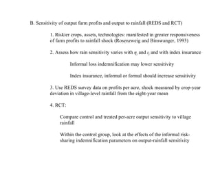
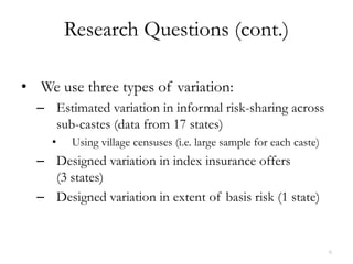
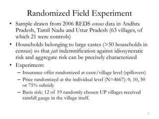
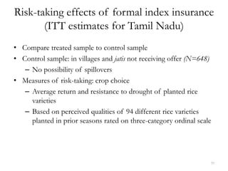
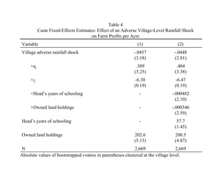
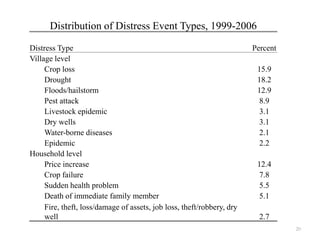
1) The document describes a field experiment that randomized offers of index insurance to agricultural households in India to study the interaction between formal insurance and informal risk-sharing networks. 2) It finds that the presence of strong informal risk-sharing networks through castes/jatis reduces demand for formal insurance, and that basis risk, where payouts do not perfectly correlate with losses, also reduces demand. 3) However, informal and formal insurance can be complements when basis risk is high, as both provide partial coverage against different risks. The study uses detailed survey and rainfall data on castes/jatis to characterize their risk-sharing practices.

1. Selling Formal Insurance to the
Informally Insured
A. Mushfiq Mobarak
Mark Rosenzweig
Yale University

2. Background
• Formal insurance markets largely absent where they
are needed
– 75% of the world’s poor engaged in agriculture
– 90% of variation in Indian agricultural production
caused by variation in rainfall
– 90% of Indians not covered by formal insurance
• Informal risk sharing networks are important
– Protects against idiosyncratic risk and perhaps aggregate
risk
– But risk-sharing is incomplete (Townsend 1994). Lower
risk-taking by farmers than we would want
– Informal risk-sharing can drive out formal insurance,
given moral hazard (Arnott and Stiglitz, 1991)
2

3. Index Insurance
• Low Incidence of Formal Crop Insurance
– Demand: Income/liquidity constraints, Trust/fraud
– Supply: High overhead costs (moral hazard, adverse
selection)
• Index-based insurance
– Payment schemes based on an exogenous publicly
observable index, such as local rainfall
– Mitigates moral hazard and adverse selection
• Arnott and Stiglitz (1991) analysis not directly relevant
– Eliminates the need for in-field assessments
– But basis risk (Clarke 2011)
– Observe low demand (Cole et al 2009, Gine and Yang
2009)
3

4. Setting and Approach
• We design a simple index insurance contract for the
Agricultural Insurance Company of India
• We randomize insurance offers to 5100 cultivators and
wage laborers across three states in India
– Wage laborers face less basis risk than cultivators
• The sub-caste (jati) is the identifiable risk-sharing network
that people are born into.
– Jatis can span districts or even states (permits aggregate risk
sharing of village rainfall shocks)
• We make offers to jatis for whom we have rich, detailed
histories of both aggregate and idiosyncratic shocks and
responsiveness to shocks.
• We randomly allocate rainfall stations to some villages.
4

5. Research Questions
1. Demand for Insurance:
– How does the presence of risk-sharing networks
affect the demand for index insurance?
2. Interaction between Index Insurance with Basis
Risk and Informal Risk Sharing:
– How important is basis risk in affecting index
insurance take-up?
3. Risk Taking:
– How does formal index insurance affect risk-taking
(in the presence of informal risk sharing)?
5

6. Research Questions (cont.)
• We use three types of variation:
– Estimated variation in informal risk-sharing across
sub-castes (data from 17 states)
• Using village censuses (i.e. large sample for each caste)
– Designed variation in index insurance offers
(3 states)
– Designed variation in extent of basis risk (1 state)
6

7. Outline
• Theory
– Index insurance with basis risk embedded in a model of
cooperative risk sharing (Arnott-Stiglitz 1991 and Clarke 2011)
– Demand for index insurance (with basis risk) by network
• (Historical) Survey Data
– Characterize jatis in terms of indemnification of
idiosyncratic and aggregate losses
– Effect of informal insurance on risk-taking
• Field Experiment
– Demand for formal insurance by different jatis
– Effect of formal index insurance on risk-taking
7

8. A-S Model of Informal Risk-sharing
• Game with two identical, cooperative partners and full
information
• Each member faces an independent adverse event with
probability P, which causes a loss d
• P can be lowered by investing in a risk-mitigating
technology e, but that also lowers w: P(e)’<0, w(e)<0.
• If a farmer incurs a loss he receives a payment δ from his
partner if the partner does not incur a loss. Thus, he also
pays out δ if his partner incurs a loss and he does not.
• Each partner chooses e and δ to maximize:
E(U) = U0(1- P)2 + U1P2 + (1 - P)P(U2 + U3),
where U0 = U(w) , U1 = U(w - d), U2 = U(w - δ), U3 = U(w - d + δ).
• Arnott-Stiglitz result: informal insurance could decrease risk taking.
8

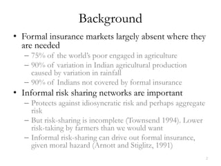
9. FOC:
e: P'[-2(1 - P)U0 + 2PU1 + (1 - 2P)(U2 + U3)] =
-w'[U0'(1- P)2 + U1'P2 + (1 - P)P(U2' + U3 ')
δ: (-U2' + U3')P(1 - P) = 0
So, optimal δ, δ*, is
δ* = d /2 where -U2' + U3 = 0 (A-S result)
9

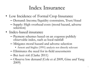
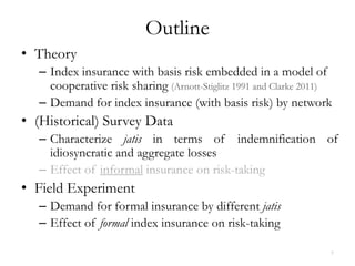
10. Aggregate Risk and Index Insurance
Now introduce a new aggregate risk and index insurance (No basis risk)
Probability that an adverse event causes losses for all participants = q
Loss from aggregate shock = L Index insurance payout = i
Actuarially-fair index insurance premium = qi
Assume q and P are independent. P is now idiosyncratic risk
E(U) = q [U0(1 - P)2 + U1P2 + (1 - P)P(U2 + U3)]
+ (1-q) [u0(1 - P)2 + u1P2 + (1 - P)P(u2 + u3)]
where U0 = U(w - L + (1 – q)i), U1 = U(w - d - L+ (1 - q)i),
U2 = U(w - δ - L + (1 -q)i), U3 = U(w - d - L + δ + (1 - q)i),
u0 = u(w - qi) , u1 = U(w - d - qi),
u2 = u(w - δ - qi), u3 = u(w - d + δ - qi)

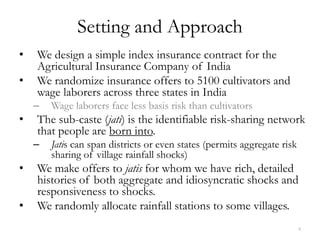
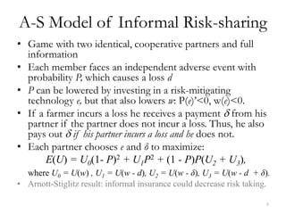
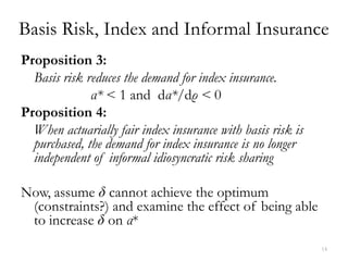
11. Proposition 2:
If there is no basis risk and index insurance is actuarially fair,
the partners will choose full index insurance. The demand for
index insurance is independent of δ.
The FOC’s for δ and i:
δ: q(-U2’+ U3’)P(1-P)+(1-q)(-u2’+u3’)P(1-P) = 0
i: q(1-q){[U0’(1-P)2+U1’P2+(U2’+U3’)P(1-P)]
+ [u0’(1-P)2+u1’P2+ (u2’+u3’)P(1-P]}=0
Thus
δ * = d/2 Optimal private individual insurance remains the same
i* = L Full index insurance (if actuarially fair) is optimal
So aggregate risk or index insurance does not affect optimal informal payout
Informal individual insurance does not crowd out index
insurance – in the absence of basis risk
Intuition: index insurance and informal risk-sharing address
two separate, independent risks.

12. Introducing Basis Risk (Clarke, 2011)
• Insurance company pays out when index passes a
threshold
• r = probability a payout is made by insurance
company
• q and r correlated imperfectly
• Basis Risk parameter ρ :
– ρ = the joint probability that there is no payout from
index insurance but each community member
experiences the loss L
• α = fraction of loss the agent chooses to indemnify
12

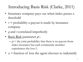
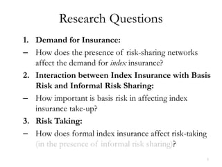
13. E(U) = (r - ρ)[U0(1 - P)2 + U1P2 + (1 - P)P(U2 + U3)]
+ ρ[u0(1 - P)2 + u1P2 + (1 - P)P(u2 + u3)]
+ (q + ρ - r)[U4(1 - P)2 + U5P2 + (1 - P)P(U6 + U7)]
+ (1 - q - ρ)[u4(1 - P)2 + u5P2 + (1 - P)P(u6 + u7)],
where
U0 = U(w - L + (1 - q)αL), U1 = U(w - d - L+ (1 - q)αL),
U2 = U(w - δ - L + (1 -q)αL), U3 = U(w - d - L + δ + (1 - q)αL),
U4 = U(w + (1 - q)αL), U5 = U(w - d + (1 - q)αL),
U6 = U(w - δ + (1 - q)αL), U7 = U(w - d + δ + (1 - q)αL), and
u0 = u(w - L(1 - qα)) , u1 = U(w - d - L(1 - qα)),
u2 = u(w - δ - L(1 - qα)), u3 = u(w - d + δ - L(1 - qα)),
u4 = u(w - qαL), u5 = U(w - d - qαL),
u6 = u(w - δ - qαL), u7 = u(w - d + δ - qαL)
13

14. Basis Risk, Index and Informal Insurance
Proposition 3:
Basis risk reduces the demand for index insurance.
α* < 1 and dα*/dρ < 0
Proposition 4:
When actuarially fair index insurance with basis risk is
purchased, the demand for index insurance is no longer
independent of informal idiosyncratic risk sharing
Now, assume δ cannot achieve the optimum
(constraints?) and examine the effect of being able
to increase δ on α*
14

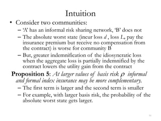
15. dα*/dδ =
{(1 - P)P{(r - ρ)(1 - q)(U3 - U2) - ρq(u3 - u 2)
+ (q + ρ - r)(1 - q)(U7 - U6) -
(1 - q - ρ)q(u7 - u6)}/Θ,
where Θ =
(1 - q)2{(r - ρ)[U0(1 - P)2 + U1P2 + (1 - P)P(U2+ U3)]
+ (q + ρ - r)[U4(1 - P)2 + U5P2 + (1 - P)P(U6 + U7)]}
+ q2{ρ[u0(1 - P)2 + u 1P2 + (1 - P)P(u2 + u 3)] + (1 - q - ρ)[u4(1 - P)2 +
u5P2 + (1 - P)P(u6 + u7)]}<0
Thus, dα*/dδ  0
but dα*/dδ can be either positive or negative
15

16. Intuition
• Consider two communities:
– ‘A’ has an informal risk sharing network, ‘B’ does not
– The absolute worst state (incur loss d , loss L, pay the
insurance premium but receive no compensation from
the contract) is worse for community B
– But, greater indemnification of the idiosyncratic loss
when the aggregate loss is partially indemnified by the
contract lowers the utility gain from the contract
Proposition 5: At larger values of basis risk ρ informal
and formal index insurance may be more complementary.
– The first term is larger and the second term is smaller
– For example, with larger basis risk, the probability of the
absolute worst state gets larger.
16

17. Implications to be Tested
• When there is no basis risk, informal idiosyncratic
coverage should not affect the demand for formal index
insurance.
• With larger basis risk, indemnification against idiosyncratic
risk and index insurance are complements.
• Index insurance can allow more risk-taking even in the
presence of informal insurance
• As wage workers face less basis risk than cultivators, a
reduction in basis risk will affect wage workers less than
cultivators
• If the informal network already provides index coverage,
that can crowd out formal index insurance.
17

18. Setting
• Advantages of data on sub-castes:
– The risk sharing network is well defined (jati)
– Exogenous (by birth, with strong penalties on inter-
marriage (<5% marry outside jati in rural India)
– Jati, not village (or geography) is the relevant risk-sharing
group. Majority (61%) of informal loans and transfers
originate outside the village.
– Depending on jati characteristics, both idiosyncratic and
aggregate risk may get indemnified to different extents.
– We have historical (REDS) data on jati identity and
transfers for a large sample (17 states, N=119,709 for
census, and N=7,342 for detailed sample survey) in
response to idiosyncratic and aggregate risks
18

19. Figure 1:Lowess-Smoothed Relationship between Inter-Village Distance (Km)
and June-August Rainfall Correlation, Andhra Pradesh and Uttar Pradesh 1999-2006
1
0.9
0.8
0.7
0.6
0.5
0.4
0.3
0.2
0.1
0
25.9
40.1
54
67.4
77.2
86.7
95
132
186
267
305
355
384
432
453
471
498
520
580

20. Key information from 2007/8 REDS
1. Amounts of “assistance received at time of difficulty”+ loans from
relatives/friends within and outside the village in 2005/6
2. Monthly rainfall in each village from 1999/2000 through 2005/6
3. History of Village-level distress events (crop loss, pest attack, drought,
cyclone/floods/hailstrorm, livestock epidemic) 1999/2000 - 2007/8
4. History of Household-specific distress events (fire, deaths of immediate
family, health problems/accidents, crop failure, theft/robbery, dry
wells) 1999/2000 - 2007/8
5. Amounts of losses from each event
6. Measures taken by household to reduce impact of events after they
occurred (crop choice, improved technology, livestock immunization)
7. Caste, land holdings, education, occupation, detail for computing farm
profits (Foster and Rosenzweig, 2011).
=> Can estimate jati responsiveness to idiosyncratic and aggregate
shocks
19

21. Distribution of Distress Event Types, 1999-2006
Distress Type Percent
Village level
Crop loss 15.9
Drought 18.2
Floods/hailstorm 12.9
Pest attack 8.9
Livestock epidemic 3.1
Dry wells 3.1
Water-borne diseases 2.1
Epidemic 2.2
Household level
Price increase 12.4
Crop failure 7.8
Sudden health problem 5.5
Death of immediate family member 5.1
Fire, theft, loss/damage of assets, job loss, theft/robbery, dry
well 2.7
20

22. 21

23. Randomized Field Experiment
• Sample drawn from 2006 REDS census data in Andhra
Pradesh, Tamil Nadu and Uttar Pradesh (63 villages, of
which 21 were controls)
• Households belonging to large castes (>50 households in
census) so that jati indemnification against idiosyncratic
risk and aggregate risk can be precisely characterized
• Experiment:
– Insurance offer randomized at caste/village level (spillovers)
– Price randomized at the individual level (N=4667): 0, 10, 50
or 75% subsidy
– Basis risk: 12 of 19 randomly chosen UP villages received
rainfall gauge in the village itself.
22

24. Delayed Monsoon Onset Insurance Product
Agricultural Insurance Company of India (AICI)
AICI offers area based and weather based crop insurance programs in almost
500 districts of India, covering almost 20 million farmers, making it one of the
biggest crop insurers in the world.
Timing and Payout Function
Trigger Range of Days Post Onset Payout (made if less than 30-40mm
Number (varied across states and (depending on state) is received at
villages) each trigger point)
1 15-20 Rs. 300
2 20-30 Rs. 750
3 25-40 Rs. 1,200
Rainfall measured at the block level from AWS (Automatic weather stations)

25. Rainfall Insurance Take-up Rates and
Average Number of Policy Units Purchased
80
70 2.6
4.9
1.6
60
50 TN
AP
1.3
40 1.38 UP
2.1
30 1.1
1.08
1.0 1.1
20
1.0
1
10
0
Discount = 0 Discount = 10% Discount = 50% Discount= 75 %
24

26. Rain per Day in 2011 Kharif Crop Season in Uttar Pradesh, by Rainfall Station
18
16
14
12
Centimeters
10
8
6
4
2
0

27. Rain per Day in 2011 Kharif Crop Season in Andhra Pradesh, by Rainfall Station
Insurance Payout Stations in Red (with Rupee Payout)
18
16
14
12
Centimeters
10
8
6
4 300
300
2 750 1200
0

28. Identifying the strength of informal, group-based
idiosyncratic and index insurance
• Need to estimate the determinants of informal indemnification δ
• Payment δijk made to household i in caste group j in village k in the
event of a household-specific loss dijk or an aggregate village
production shock ζk
δijk = ηij dijk +ιij ζk + μj where ηij= η(Xj, Xij), ιij= ι(Xj, Xij )
• Indemnification of shocks depends on caste and household
characteristics.
• What are the relevant caste-level variables that affect the ability to
pool risk?
– Group’s ability to indemnify risk and avoid moral hazard depends on the
group’s level of resources, its ability to agree on common actions, its ability to
diversify risk, and its ability to monitor.
27

29. Estimate the effect of informal insurance on
formal index insurance demand
• Compute from the estimates caste-specific (and household-
specific) abilities to indemnify against
actual individual losses: ηj = ΣηjnXjn
aggregate shocks (index) ιij = Σ ι jnXjn
• Use estimates as determinants of formal insurance take-up
• Bootstrap standard errors (1,000 draws) clustered at caste level.
28

30. Estimation of ηj and ιij
• Problem:
– Household losses have a caste-level component:(dijk + dj)
– Arnott-Stiglitz model indicates that risk-taking is endogenous
at the sub-caste level
– Other unobserved caste-level characteristics might also matter.
• Solution:
– Can estimate the interaction parameters ηjn and iim even after
adding caste-fixed effects to eliminate, dj , μj (and any
unmeasured differences across Indian states)
– Cannot identify the effect of caste variables on the level of
transfers, but they are not of direct interest here
– Caste fixed-effects accounts for other caste unobservables
such as average risk aversion or how close knit the community
is on average transfers
29

31. Bias from Moral Hazard
• Schulhofer-Wohl (JPE 2012) and Mazzocco and Saini (AER
2011) argue that individual losses are correlated with individual
preferences for risk, and this biases consumption/income-type
tests of risk sharing.
• Unlike this literature, we use direct data on transfers in
response to shocks (not income-consumption co-movements).
• However, larger transfers may lead to moral hazard, and
individuals face greater shocks as a result
– This cannot be true of village-level rainfall shocks (since village
location choices are unlikely to be endogenous in this context)
– Arnott-Stiglitz model assumes that the network monitors moral
hazard, so this is not true in the model within castes
– Caste (jati) fixed effect absorbs differences across castes in risk-
taking
Hausman test: uses rainfall shocks interacted with household characteristics to
predict hh losses; cannot reject exogeneity (net of caste fixed effect)
30

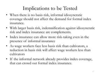
32. Response to Aggregate Risk
ML Conditional Logit Estimates of the Determinants of Receiving Financial Assistance
(Informal Loans + Non-regular Transfers in Crop Year 2005/6)
Variable/Coefficient type Log-Odds P Log-Odds P
-0.00183 -0.00046 -0.00179 0.00045
Adverse village rain deviation in 05/06
[2.41] [2.41] [2.35] [2.35]
0.000256 0.00006 0.000274 0.00007
×Caste’s mean land holdings
[1.64] [1.64] [1.71] [1.71]
0.00139 0.00035 0.00165 0.00041
×Caste’s proportion landless
[1.35] [1.35] [1.68] [1.68]
×Caste’s proportion hh’s with in non-ag. 0.0206 0.00513 0.0207 0.0052
occupations [3.29] [3.29] [3.32] [3.32]
×Caste’s standard deviation of land -0.00232 0.000579 -0.00426 0.0011
holdings (x10-3) [0.18] [0.18] [0.32] [0.32]
×Number of same-caste households in 0.00109 -0.000273 0.00114 0.00028
village (x10-3) [0.90] [0.90] [0.93] [0.93]
31

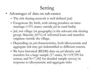
33. Response to Idiosyncratic Risk
-0.833 -0.204251 -0.794 -0.195
Any individual household loss from distress event in 05/06
[2.49] [2.61] [2.38] [2.48]
0.144 0.036024 0.165 0.0412
×Caste’s mean land holdings
[1.68] [1.68] [1.98] [1.98]
1.37 0.341520 1.22 0.305
×Caste’s proportion landless
[2.40] [2.40] [2.01] [2.01]
3.05 0.761193 3.25 0.81
×Caste’s proportion hh’s with in non-ag. occupations
[1.47] [1.47] [1.53] [1.53]
-16.5 -4.1194 -18.8 -4.69
×Caste’s standard deviation of land holdings (x10-3)
[1.84] [1.84] [2.12] [2.12]
1.77 0.4415 1.73 0.00043
×Number of same-caste households in village (x10-3)
[2.38] [2.38] [2.37] [2.37]
32

34. Is there basis risk in this sample?
Variable Uttar Pradesh (randomized) UP+AP
Rain per day 0.16516 0.30169 0.13937 0.23606
[1.32] [2.20] [1.40] [2.09]
Distance to aws (km) 0.12483 0.08460
[2.40] [1.92]
Rain per day x Distance to aws -0.02231 -0.01673
[3.53] [2.81]
Number of cultivators 945 936 1,459 1,418
33

35. Figure 1: Lowess-Smoothed Relationship Between Log Output Value per Acre and Log Rain
in the Kharif Season, by Randomized Placement of Rain Station (UP Villages)
13
12
11
10
AWS Outside Village
9
AWS in Village
8
7
6
1.8 1.9 2 2.1 2.2 2.3 2.4 2.5 2.6

36. Fixed-Effects Estimates: Determinants of Formal Insurance Take-up (bootstrapped t -ratios)
FE-State FE-Caste
Three Two States Two States
Variable/Est. Method States (AP and UP) UP only AP only (AP and UP)
0.125 0.151 0.0228 -0.523 -0.029 - -
η j [Informal idiosyncratic coverage]
[0.56] [0.61] [0.07] [0.73] [0.06]
- - 0.151 0.174 0.153 0.139 0.157
η j × Distance to AWS
[3.42] [1.34] [1.16] [2.55] [2.31]
-198 -209.6 -209.7 -78.2 -121.7 - -
ι j [Informal aggregate coverage]
[1.71] [1.28] [0.94] [0.48] [0.33]
- - - - - - -18.6
ι j × Distance to AWS
[-0.528]
- - -0.0254 -0.029 -0.025 -0.0246 -0.019
Distance to AWS (km)
[3.50] [1.67] [0.90] [2.63] [1.50]
-0.0343 -0.0341 -0.028 -0.047 -0.018 -0.0238 -0.0379
Agricultural laborer
[2.19] [2.13] [1.58] [1.41] [0.92] [1.49] [1.43]
Agricultural laborer × Distance - - - - - - 0.0033
to aws [0.797]
-0.00143 -0.0016 -0.0017 -0.003 -0.001 -0.0015 -0.0016
Actuarial price
[2.07] [2.07] [2.40] [1.46] [1.81] [2.14] [2.14]
0.389 0.355 0.35 0.187 0.447 0.376 0.372
Subsidy
[3.38] [2.86] [3.10] [0.68] [3.95] [3.26] [3.20]
Village coefficient of variation, 0.523 0.751 0.747 1.050 0.267 0.874 0.908
rainfall [2.16] [2.89] [2.77] [2.93] [0.46] [2.92] [3.04]
N 4,260 3,338 3,338 1,693 1,645 3,338 3,338

37. Is it Trust?
• Perhaps distance to the rain station (village
presence) allows respondents to trust that they
will get a payment
• Lack of trust, when asked why did not purchase,
was not a salient issue
• Probability that farmers mentioned trust as an
issue in non-purchase not correlated with
distance (multinomial logit estimates for
purchase versus not purchase by reason)
36

38. Reasons
Table 8
Reasons Given for Not Purchasing Marketed Insurance,
by Cultivator Status
Variable Cultivator (%) Non-cultivator (%)
Too expensive 2.26 1.32
Currently not holding cash 45.4 49.7
No need 35.5 38.8
Do not trust insurance/payout
unlikely 13.8 9.62
Do not understand 3.02 0.62
37

39. AWS Distance and Trust
Table 9
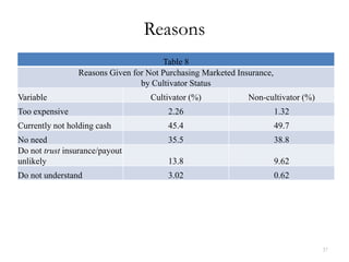
Marginal Effects from Multinomial Logit Regression of Reasons for not Purchasing Insurance
[bootstrapped t-ratios]
Purchased Insurance Lack of Trust
-0.034 0.080
ηj
[0.23] [1.64]
0.200 0.007
ηj × Distance to aws
[3.40] [0.55]
213.879 14.481
ιj
[1.30] [0.33]
ιj × Distance to aws
-0.036 0.000
Distance to aws (km)
[3.67] [0.08]
38

40. Risk-taking effects of formal index insurance
(ITT estimates for Tamil Nadu)
• Compare treated sample to control sample
• Control sample: in villages and jatis not receiving offer (N=648)
– No possibility of spillovers
• Measures of risk-taking: crop choice
– Average return and resistance to drought of planted rice
varieties
– Based on perceived qualities of 94 different rice varieties
planted in prior seasons rated on three-category ordinal scale
39

41. The index for yield and drought resistance is
Ili = Σaisσls/Σais
where
l is drought resistance or yield
σls = fraction of all farmers rating rice variety s “good” with
respect to the characteristic l
ais=acreage of rice variety s planted by farmer I
Median rice portfolio: 57% “good” for yield, 63% “good” for
tolerance
Only 5% of farmers planted varieties considered
“good” for yield by every farmer
Only 9% of farmers planted varieties considered
“good” for drought resilience by all farmers
40

42. Properties of Rice Varieties Planted by Tamil Nadu Rice Farmers
Drought Disease Insect
Property Yield Resistant Resistant Resistant
Good 61.0 58.9 40.3 34.7
Neither good nor poor 30.7 30.9 46.2 50.6
Poor 8.3 10.2 13.5 14.7
Total 100.0 100.0 100.0 100.0
Number of varieties 94
Number of farmers 364
41

43. Estimating equation:
Ili = gωlωi + gωlηωiηj + gωlιωiιj + x ijg + gj + εij
where
ωi = 1 if the index insurance product was offered to
the farmer
gj = caste fixed effect
εij is an iid error
Model suggests that
gωl>0 for l=drought resistance
gωl<0 for l=yield
42

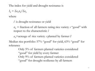
44. Intent-to-Treat Caste Fixed-Effects Estimates of Index Insurance on Risk and Yield:
Proportion of Planted Crop Varieties Rated "Good" for Drought Tolerance and Yield, Tamil Nadu
Kharif Rice Farmers
Crop Characteristic: Good Drought Tolerance Good Yield
Variable (1) (1)
Offered insurance -0.0593 0.0519
[2.67] [1.93]
Owned land holdings 0.0000934 0.00056
[0.02] [0.12]
Village coefficient of variation, r 0.351 -0.516
[0.88] [0.81]
N 325 325
Absolute values of t-ratios in brackets, clustered by caste/village (because the randomized insurance
treatment was stratified at the caste/village level).

45. Conclusions
• Informal networks lower the demand for formal
insurance only if the network covers aggregate risk.
• When formal insurance carries basis risk, informal
risk sharing can be a complement to formal
insurance
• Formal insurance enables households to take more
risk, and thus assists in income growth.
• Landless laborers’ livelihoods are weather
dependent, and they also demonstrate a strong
demand for insurance, especially relative to
cultivators living farther away from rainfall stations.
45

46. What is the relationship between risk-taking and
A. Weather Insurance
B. Informal Loss Indemnification
Theory
Empirical findings using rainfall variation:
A. NCAER REDS 2007-8 cultivators
1. Informal jati-level indemnification estimates and rainfall
deviations from 8-year mean
B. RCT in Andhra Pradesh and Uttar Pradesh - cultivators
1. Informal jati-level indemnification estimates
2. Randomized weather insurance

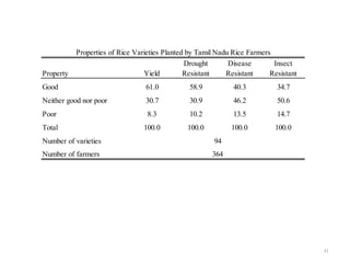
47. Partners behave cooperatively, choosing e and ä to maximize:
E(U) = U0(1- P)2 + U1P2 + (1 - P)P(U2 + U3),
where U0 = U(w) , U1 = U(w - d), U2 = U(w - ä), U3 = U(w - d + ä)
FOC:
e: P'[-2(1 - P)U0 + 2PU1 + (1 - 2P)(U2 + U3)] =
-w'[U0'(1- P)2 + U1'P2 + (1 - P)P(U2' + U3')
ä: (-U2' + U3')P(1 - P) = 0
So, optimal ä, ä*, is
ä* = d /2 where -U2' + U3 = 0 (A-S result)
Suppose that the group cannot attain “full” insurance ä*(limited commitment,
liquidity constraints), so that ä < ä*.

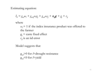
48. What is the effect of exogenous fall in ä at the optimum ä*, on risk mitigation
e?
Proposition 1: A decrease in the ability to informally indemnify individual
losses below the first-best constrained optimum, may increase risk-taking.
de/dä = -[(1 - 2P)(U2' + U3')P'+ (1 - P)P(-U2" + U3")w"]/Ö,
where Ö = (w')2[U0"(1 - P)2 + U1"P2 + (1 - P)P(U2" + U3")]
+ [U0'(1 - P)2 + U1'P2 + (1 - P)P(U2' + U3')][w" - P"W'/P']
+ 2(P')2[U0 + U1 - U2 - U3] < 0
and -U2' + U3 > 0, -U2" + U3"<0 for ä < ä*
For P $ ½, decreased coverage unambiguously decreases risk-mitigation,
but below ½, the effect may be negative as well.
More effective informal risk-sharing may be associated with lower risk-taking

49. B. Sensitivity of output farm profits and output to rainfall (REDS and RCT)
1. Riskier crops, assets, technologies: manifested in greater responsiveness
of farm profits to rainfall shock (Rosenzweig and Binswanger, 1993)
2. Assess how rain sensitivity varies with çj and éj and with index insurance
Informal loss indemnification may lower sensitivity
Index insurance, informal or formal should increase sensitivity
3. Use REDS survey data on profits per acre, shock measured by crop-year
deviation in village-level rainfall from the eight-year mean
4. RCT:
Compare control and treated per-acre output sensitivity to village
rainfall
Within the control group, look at the effects of the informal risk-
sharing indemnification parameters on output-rainfall sensitivity

50. Table 4
Caste Fixed-Effects Estimates: Effect of an Adverse Village-Level Rainfall Shock
on Farm Profits per Acre
Variable (1) (2)
Village adverse rainfall shock -.0457 -.0448
(3.18) (2.81)
×çj .389 .404
(3.25) (3.38)
×éj -6.30 -6.47
(0.19) (0.19)
×Head’s years of schooling - -.000482
(2.10)
×Owned land holdings - -.000346
(2.59)
Head’s years of schooling - 57.7
(1.45)
Owned land holdings 202.6 200.5
(5.13) (4.87)
N 2,669 2,669
Absolute values of bootstrapped t-ratios in parentheses clustered at the village level.

51. Figure 6: Lowess-Smoothed Relationship Between Log Per-Acre Output Value
and Log Rain per Day in the Kharif Season, by Insurance Type and Level
11
10.5
10
9.5
9
8.5
High Informal Indemnification, No Rainfall Insurance
8
Low Informal Indemnification, No Rainfall Insurance
Offered Rainfall Insurance
7.5
7
0.75 1.25 1.75 2.25 2.75