SlideShare a Scribd company logo
1 of 103
• Linear Regression in Machine Learning
• Linear regression is one of the easiest and most popular Machine Learning algorithms. It is a
statistical method that is used for predictive analysis. Linear regression makes predictions for
continuous/real or numeric variables such as sales, salary, age, product price, etc.
• Linear regression algorithm shows a linear relationship between a dependent (y) and one or
more independent (y) variables, hence called as linear regression. Since linear regression
shows the linear relationship, which means it finds how the value of the dependent variable is
changing according to the value of the independent variable.
• The linear regression model provides a sloped straight line representing the relationship
between the variables. Consider the below image:
•
• Mathematically, we can represent a linear regression as:
• y= a0+a1x+ ε
• Here,
• Y= Dependent Variable (Target Variable)
X= Independent Variable (predictor Variable)
a0= intercept of the line (Gives an additional degree of freedom)
a1 = Linear regression coefficient (scale factor to each input value).
ε = random error
• The values for x and y variables are training datasets for Linear Regression model
representation.
• Types of Linear Regression
• Linear regression can be further divided into two types of the algorithm:
• Simple Linear Regression:
If a single independent variable is used to predict the value of a numerical dependent variable,
then such a Linear Regression algorithm is called Simple Linear Regression.
• Multiple Linear regression:
If more than one independent variable is used to predict the value of a numerical dependent
variable, then such a Linear Regression algorithm is called Multiple Linear Regression.
• Linear Regression Line
• A linear line showing the relationship between the dependent and
independent variables is called a regression line. A regression line can show
two types of relationship:
• Positive Linear Relationship:
If the dependent variable increases on the Y-axis and independent variable
increases on X-axis, then such a relationship is termed as a Positive linear
relationship.
• Negative Linear Relationship:
If the dependent variable decreases on the Y-axis and independent variable increases on the X-
axis, then such a relationship is called a negative linear relationship.
• Finding the best fit line:
• When working with linear regression, our main goal is to find the best fit line that
means the error between predicted values and actual values should be minimized. The
best fit line will have the least error.
• The different values for weights or the coefficient of lines (a0, a1) gives a different line
of regression, so we need to calculate the best values for a0 and a1 to find the best fit
line, so to calculate this we use cost function.
• Cost function-
• The different values for weights or coefficient of lines (a0, a1) gives the different
line of regression, and the cost function is used to estimate the values of the
coefficient for the best fit line.
• Cost function optimizes the regression coefficients or weights. It measures how
a linear regression model is performing.
• We can use the cost function to find the accuracy of the mapping function,
which maps the input variable to the output variable. This mapping function is
also known as Hypothesis function.
• For Linear Regression, we use the Mean Squared Error (MSE) cost function,
which is the average of squared error occurred between the predicted values
and actual values. It can be written as:
• For the above linear equation, MSE can be calculated as:
N=Total number of observation
Yi = Actual value
(a1xi+a0)= Predicted value.
Residuals: The distance between the actual value and predicted values is called
residual. If the observed points are far from the regression line, then the residual will
be high, and so cost function will high. If the scatter points are close to the regression
line, then the residual will be small and hence the cost function.
• Gradient Descent:
• Gradient descent is used to minimize the MSE by calculating the gradient of the cost
function.
• A regression model uses gradient descent to update the coefficients of the line by
reducing the cost function.
• It is done by a random selection of values of coefficient and then iteratively update the
values to reach the minimum cost function.
• Model Performance:
• The Goodness of fit determines how the line of regression fits the set of observations.
The process of finding the best model out of various models is called optimization. It
can be achieved by below method:
• R-squared method:
• R-squared is a statistical method that determines the goodness of fit.
• It measures the strength of the relationship between the dependent and
independent variables on a scale of 0-100%.
• The high value of R-square determines the less difference between the
predicted values and actual values and hence represents a good model.
• It is also called a coefficient of determination, or coefficient of multiple
determination for multiple regression.
• It can be calculated from the below formula:
• Assumptions of Linear Regression
• Below are some important assumptions of Linear Regression. These are some
formal checks while building a Linear Regression model, which ensures to get
the best possible result from the given dataset.
• Linear relationship between the features and target:
Linear regression assumes the linear relationship between the dependent and
independent variables.
• Small or no multicollinearity between the features:
Multicollinearity means high-correlation between the independent variables.
Due to multicollinearity, it may difficult to find the true relationship between
the predictors and target variables. Or we can say, it is difficult to determine
which predictor variable is affecting the target variable and which is not. So,
the model assumes either little or no multicollinearity between the features or
independent variables.
• Homoscedasticity Assumption:
Homoscedasticity is a situation when the error term is the same for all the values
of independent variables. With homoscedasticity, there should be no clear
pattern distribution of data in the scatter plot.
• Normal distribution of error terms:
Linear regression assumes that the error term should follow the normal
distribution pattern. If error terms are not normally distributed, then confidence
intervals will become either too wide or too narrow, which may cause difficulties
in finding coefficients.
It can be checked using the q-q plot. If the plot shows a straight line without any
deviation, which means the error is normally distributed.
• No autocorrelations:
The linear regression model assumes no autocorrelation in error terms. If there
will be any correlation in the error term, then it will drastically reduce the
accuracy of the model. Autocorrelation usually occurs if there is a dependency
between residual errors.
• Simple Linear Regression in Machine Learning
• Simple Linear Regression is a type of Regression algorithms that models the
relationship between a dependent variable and a single independent variable. The
relationship shown by a Simple Linear Regression model is linear or a sloped straight
line, hence it is called Simple Linear Regression.
• The key point in Simple Linear Regression is that the dependent variable must be a
continuous/real value. However, the independent variable can be measured on
continuous or categorical values.
• Simple Linear regression algorithm has mainly two objectives:
• Model the relationship between the two variables. Such as the relationship between
Income and expenditure, experience and Salary, etc.
• Forecasting new observations. Such as Weather forecasting according to
temperature, Revenue of a company according to the investments in a year, etc.
• Simple Linear Regression Model:
• The Simple Linear Regression model can be represented using the below equation:
• y= a0+a1x+ ε
• Where,
• a0= It is the intercept of the Regression line (can be obtained putting x=0)
a1= It is the slope of the regression line, which tells whether the line is
increasing or decreasing.
ε = The error term. (For a good model it will be negligible)
• Implementation of Simple Linear Regression Algorithm using Python
• Problem Statement example for Simple Linear Regression:
• Here we are taking a dataset that has two variables: salary (dependent variable)
and experience (Independent variable). The goals of this problem is:
• We want to find out if there is any correlation between these two variables
• We will find the best fit line for the dataset.
• How the dependent variable is changing by changing the independent
variable.
• In this section, we will create a Simple Linear Regression model to find out the
best fitting line for representing the relationship between these two variables.
• To implement the Simple Linear regression model in machine learning using
Python, we need to follow the below steps:
• Step-1: Data Pre-processing
• The first step for creating the Simple Linear Regression model is data pre-processing.
We have already done it earlier in this tutorial. But there will be some changes, which
are given in the below steps:
• First, we will import the three important libraries, which will help us for loading
the dataset, plotting the graphs, and creating the Simple Linear Regression
model.
• import numpy as nm
• import matplotlib.pyplot as mtp
• import pandas as pd
• Next, we will load the dataset into our code:
• data_set= pd.read_csv('Salary_Data.csv')
• By executing the above line of code (ctrl+ENTER), we can read the dataset on our
Spyder IDE screen by clicking on the variable explorer option.
• The above output shows the dataset, which has two variables: Salary and Experience.
• Note: In Spyder IDE, the folder containing the code file must be saved as a working
directory, and the dataset or csv file should be in the same folder.
• After that, we need to extract the dependent and independent variables from the given
dataset. The independent variable is years of experience, and the dependent variable is
salary. Below is code for it:
• x= data_set.iloc[:, :-1].values
• y= data_set.iloc[:, 1].values
• In the above lines of code, for x variable, we have taken -1 value since we want
to remove the last column from the dataset. For y variable, we have taken 1
value as a parameter, since we want to extract the second column and indexing
starts from the zero.
• By executing the above line of code, we will get the output for X and Y variable
as:
• In the above output image, we can see the X (independent) variable and Y (dependent)
variable has been extracted from the given dataset.
• Next, we will split both variables into the test set and training set. We have 30
observations, so we will take 20 observations for the training set and 10 observations
for the test set. We are splitting our dataset so that we can train our model using a
training dataset and then test the model using a test dataset. The code for this is given
below:
• # Splitting the dataset into training and test set.
• from sklearn.model_selection import train_test_split
• x_train, x_test, y_train, y_test= train_test_split(x, y, test_size= 1/3, random_stat
e=0)
• By executing the above code, we will get x-test, x-train and y-test, y-train dataset.
Consider the below images:
• Test-dataset:
• Training Dataset:
• For simple linear Regression, we will not use Feature Scaling. Because Python
libraries take care of it for some cases, so we don't need to perform it here. Now, our
dataset is well prepared to work on it and we are going to start building a Simple
Linear Regression model for the given problem.
• Step-2: Fitting the Simple Linear Regression to the Training Set:
• Now the second step is to fit our model to the training dataset. To do so, we will
import the LinearRegression class of the linear_model library from the scikit learn.
After importing the class, we are going to create an object of the class named as
a regressor. The code for this is given below:
1.#Fitting the Simple Linear Regression model to the training dataset
2.from sklearn.linear_model import LinearRegression
3.regressor= LinearRegression()
4.regressor.fit(x_train, y_train)
• In the above code, we have used a fit() method to fit our Simple Linear Regression
object to the training set. In the fit() function, we have passed the x_train and y_train,
which is our training dataset for the dependent and an independent variable. We have
fitted our regressor object to the training set so that the model can easily learn the
correlations between the predictor and target variables. After executing the above lines
of code, we will get the below output.
• Output:
• Out[7]: LinearRegression(copy_X=True, fit_intercept=True, n_jobs=None,
normalize=False)
• Step: 3. Prediction of test set result:
• dependent (salary) and an independent variable (Experience). So, now, our model is
ready to predict the output for the new observations. In this step, we will provide the
test dataset (new observations) to the model to check whether it can predict the correct
output or not.
• We will create a prediction vector y_pred, and x_pred, which will contain predictions
of test dataset, and prediction of training set respectively.
• #Prediction of Test and Training set result
• y_pred= regressor.predict(x_test)
• x_pred= regressor.predict(x_train)
• On executing the above lines of code, two variables named y_pred and x_pred
will generate in the variable explorer options that contain salary predictions for
the training set and test set.
• You can check the variable by clicking on the variable explorer option in the IDE,
and also compare the result by comparing values from y_pred and y_test. By
comparing these values, we can check how good our model is performing.
• Step: 4. visualizing the Training set results:
• Now in this step, we will visualize the training set result. To do so, we will use
the scatter() function of the pyplot library, which we have already imported in
the pre-processing step. The scatter () function will create a scatter plot of
observations.
• In the x-axis, we will plot the Years of Experience of employees and on the y-
axis, salary of employees. In the function, we will pass the real values of training
set, which means a year of experience x_train, training set of Salaries y_train,
and color of the observations. Here we are taking a green color for the
observation, but it can be any color as per the choice.
• Now, we need to plot the regression line, so for this, we will use the plot() function of
the pyplot library. In this function, we will pass the years of experience for training
set, predicted salary for training set x_pred, and color of the line.
• Next, we will give the title for the plot. So here, we will use the title() function of
the pyplot library and pass the name ("Salary vs Experience (Training Dataset)".
• After that, we will assign labels for x-axis and y-axis using xlabel() and ylabel()
function.
• Finally, we will represent all above things in a graph using show(). The code is given
below:
• mtp.scatter(x_train, y_train, color="green")
• mtp.plot(x_train, x_pred, color="red")
• mtp.title("Salary vs Experience (Training Dataset)")
• mtp.xlabel("Years of Experience")
• mtp.ylabel("Salary(In Rupees)")
• mtp.show()
• Output:
• By executing the above lines of code, we will get the below graph plot as an
output.
•
• In the above plot, we can see the real values observations in green dots and predicted
values are covered by the red regression line. The regression line shows a correlation
between the dependent and independent variable.
• The good fit of the line can be observed by calculating the difference between actual
values and predicted values. But as we can see in the above plot, most of the
observations are close to the regression line, hence our model is good for the
training set.
• Step: 5. visualizing the Test set results:
• In the previous step, we have visualized the performance of our model on the training
set. Now, we will do the same for the Test set. The complete code will remain the same
as the above code, except in this, we will use x_test, and y_test instead of x_train and
y_train.
• Here we are also changing the color of observations and regression line to differentiate
between the two plots, but it is optional.
• #visualizing the Test set results
• mtp.scatter(x_test, y_test, color="blue")
• mtp.plot(x_train, x_pred, color="red")
• mtp.title("Salary vs Experience (Test Dataset)")
• mtp.xlabel("Years of Experience")
• mtp.ylabel("Salary(In Rupees)")
• mtp.show()
• Output:
• By executing the above line of code, we will get the output as:
•
• In the above plot, there are observations given by the blue color, and prediction is
given by the red regression line. As we can see, most of the observations are close to
the regression line, hence we can say our Simple Linear Regression is a good model
and able to make good predictions.
•Multiple Linear Regression
• In the previous topic, we have learned about Simple Linear Regression, where a single
Independent/Predictor(X) variable is used to model the response variable (Y). But
there may be various cases in which the response variable is affected by more than one
predictor variable; for such cases, the Multiple Linear Regression algorithm is used.
• Moreover, Multiple Linear Regression is an extension of Simple Linear regression as
it takes more than one predictor variable to predict the response variable. We can
define it as:
• Multiple Linear Regression is one of the important regression algorithms which
models the linear relationship between a single dependent continuous variable
and more than one independent variable.
• Example:
• Prediction of CO2 emission based on engine size and number of cylinders in a
car.
• Some key points about MLR:
• For MLR, the dependent or target variable(Y) must be the continuous/real, but
the predictor or independent variable may be of continuous or categorical
form.
• Each feature variable must model the linear relationship with the dependent
variable.
• MLR tries to fit a regression line through a multidimensional space of data-
points.
• MLR equation:
• In Multiple Linear Regression, the target variable(Y) is a linear combination of
multiple predictor variables x1, x2, x3, ...,xn. Since it is an enhancement of Simple
Linear Regression, so the same is applied for the multiple linear regression
equation, the equation becomes:
• Y= b<sub>0</sub>+b<sub>1</sub>x<sub>1</sub>+ b<sub>2</sub>x<sub>2</s
ub>+ b<sub>3</sub>x<sub>3</sub>+...... bnxn …….. (a)
• Where,
• Y= Output/Response variable
• b0, b1, b2, b3 , bn....= Coefficients of the model.
• x1, x2, x3, x4,...= Various Independent/feature variable
• Assumptions for Multiple Linear Regression:
• A linear relationship should exist between the Target and predictor variables.
• The regression residuals must be normally distributed.
• MLR assumes little or no multicollinearity (correlation between the
independent variable) in data.
• Implementation of Multiple Linear Regression model using Python:
• To implement MLR using Python, we have below problem:
• Problem Description:
• We have a dataset of 50 start-up companies. This dataset contains five main
information: R&D Spend, Administration Spend, Marketing Spend, State, and
Profit for a financial year. Our goal is to create a model that can easily
determine which company has a maximum profit, and which is the most
affecting factor for the profit of a company.
• Since we need to find the Profit, so it is the dependent variable, and the other
four variables are independent variables. Below are the main steps of deploying
the MLR model:
• Data Pre-processing Steps
• Fitting the MLR model to the training set
• Predicting the result of the test set
• Step-1: Data Pre-processing Step:
• The very first step is data pre-processing, which we have already discussed in this
tutorial. This process contains the below steps:
• Importing libraries: Firstly we will import the library which will help in building the
model. Below is the code for it:
• # importing libraries
• import numpy as nm
• import matplotlib.pyplot as mtp
• import pandas as pd
• Importing dataset: Now we will import the dataset(50_CompList), which
contains all the variables. Below is the code for it:
• #importing datasets
• data_set= pd.read_csv('50_CompList.csv')
• Output: We will get the dataset as:
• In above output, we can clearly see that there are five variables, in which four
variables are continuous and one is categorical variable.
• Extracting dependent and independent Variables:
• #Extracting Independent and dependent Variable
• x= data_set.iloc[:, :-1].values
• y= data_set.iloc[:, 4].values
• Output:
• Out[5]:
• rray([[165349.2, 136897.8, 471784.1, 'New York'],
• [162597.7, 151377.59, 443898.53, 'California'],
• [153441.51, 101145.55, 407934.54, 'Florida'],
• [144372.41, 118671.85, 383199.62, 'New York'],
• [142107.34, 91391.77, 366168.42, 'Florida'],
• [131876.9, 99814.71, 362861.36, 'New York'],
• [134615.46, 147198.87, 127716.82, 'California'],
• [130298.13, 145530.06, 323876.68, 'Florida'],
• [120542.52, 148718.95, 311613.29, 'New York'],
• [123334.88, 108679.17, 304981.62, 'California'],
• [101913.08, 110594.11, 229160.95, 'Florida'],
• [100671.96, 91790.61, 249744.55, 'California'],
• [93863.75, 127320.38, 249839.44, 'Florida'],
• [91992.39, 135495.07, 252664.93, 'California'],
• [119943.24, 156547.42, 256512.92, 'Florida'],
• [114523.61, 122616.84, 261776.23, 'New York'],
• [78013.11, 121597.55, 264346.06, 'California'],
• [94657.16, 145077.58, 282574.31, 'New York'],
• [91749.16, 114175.79, 294919.57, 'Florida'],
• [86419.7, 153514.11, 0.0, 'New York'],
• [76253.86, 113867.3, 298664.47, 'California'],
• [78389.47, 153773.43, 299737.29, 'New York'],
• [73994.56, 122782.75, 303319.26, 'Florida'],
• [67532.53, 105751.03, 304768.73, 'Florida'],
• [77044.01, 99281.34, 140574.81, 'New York'],
• [64664.71, 139553.16, 137962.62, 'California'],
• [75328.87, 144135.98, 134050.07, 'Florida'],
• [72107.6, 127864.55, 353183.81, 'New York'],
• [66051.52, 182645.56, 118148.2, 'Florida'],
• [65605.48, 153032.06, 107138.38, 'New York'],
• [61994.48, 115641.28, 91131.24, 'Florida'],
• [61136.38, 152701.92, 88218.23, 'New York'],
• [63408.86, 129219.61, 46085.25, 'California'],
• [55493.95, 103057.49, 214634.81, 'Florida'],
• [46426.07, 157693.92, 210797.67, 'California'],
• [46014.02, 85047.44, 205517.64, 'New York'],
• [28663.76, 127056.21, 201126.82, 'Florida'],
• [44069.95, 51283.14, 197029.42, 'California'],
• [20229.59, 65947.93, 185265.1, 'New York'],
• [38558.51, 82982.09, 174999.3, 'California'],
• [28754.33, 118546.05, 172795.67, 'California'],
• [27892.92, 84710.77, 164470.71, 'Florida'],
• [23640.93, 96189.63, 148001.11, 'California'],
• [15505.73, 127382.3, 35534.17, 'New York'],
• [22177.74, 154806.14, 28334.72, 'California'],
• [1000.23, 124153.04, 1903.93, 'New York'],
• [1315.46, 115816.21, 297114.46, 'Florida'],
• [0.0, 135426.92, 0.0, 'California'],
• [542.05, 51743.15, 0.0, 'New York'],
• [0.0, 116983.8, 45173.06, 'California']], dtype=object)
• As we can see in the above output, the last column contains categorical
variables which are not suitable to apply directly for fitting the model. So we
need to encode this variable.
• Encoding Dummy Variables:
• As we have one categorical variable (State), which cannot be directly applied to
the model, so we will encode it. To encode the categorical variable into
numbers, we will use the LabelEncoder class. But it is not sufficient because it
still has some relational order, which may create a wrong model. So in order to
remove this problem, we will use OneHotEncoder, which will create the
dummy variables. Below is code for it:
• #Catgorical data
• from sklearn.preprocessing import LabelEncoder, OneHotEncoder
• labelencoder_x= LabelEncoder()
• x[:, 3]= labelencoder_x.fit_transform(x[:,3])
• onehotencoder= OneHotEncoder(categorical_features= [3])
• x= onehotencoder.fit_transform(x).toarray()
• Here we are only encoding one independent variable, which is state as other
variables are continuous.
• As we can see in the above output, the state column has been converted into
dummy variables (0 and 1). Here each dummy variable column is
corresponding to the one State. We can check by comparing it with the
original dataset. The first column corresponds to the California State, the
second column corresponds to the Florida State, and the third column
corresponds to the New York State.
• Note: We should not use all the dummy variables at the same time, so it must
be 1 less than the total number of dummy variables, else it will create a
dummy variable trap.
• Now, we are writing a single line of code just to avoid the dummy variable trap:
• #avoiding the dummy variable trap:
• x = x[:, 1:]
• If we do not remove the first dummy variable, then it may introduce
multicollinearity in the model.
• As we can see in the above output image, the first column has been removed.
• Now we will split the dataset into training and test set. The code for this is given
below:
• # Splitting the dataset into training and test set.
• from sklearn.model_selection import train_test_split
• x_train, x_test, y_train, y_test= train_test_split(x, y, test_size= 0.2, random_stat
e=0)
• The above code will split our dataset into a training set and test set.
• Output: The above code will split the dataset into training set and test set. You
can check the output by clicking on the variable explorer option given in Spyder
IDE. The test set and training set will look like the below image:
Test set:
Training set:
• Note: In MLR, we will not do feature scaling as it is taken care by the library, so we
don't need to do it manually.
• Step: 2- Fitting our MLR model to the Training set:
• Now, we have well prepared our dataset in order to provide training, which means we
will fit our regression model to the training set. It will be similar to as we did
in Simple Linear Regression model. The code for this will be:
• #Fitting the MLR model to the training set:
• from sklearn.linear_model import LinearRegression
• regressor= LinearRegression()
• regressor.fit(x_train, y_train)
• Out[9]: LinearRegression(copy_X=True, fit_intercept=True, n_jobs=None,
normalize=False)
• Now, we have successfully trained our model using the training dataset. In the
next step, we will test the performance of the model using the test dataset.
• Step: 3- Prediction of Test set results:
• The last step for our model is checking the performance of the model. We will
do it by predicting the test set result. For prediction, we will create
a y_pred vector. Below is the code for it:
• #Predicting the Test set result;
• y_pred= regressor.predict(x_test)
• By executing the above lines of code, a new vector will be generated under the
variable explorer option. We can test our model by comparing the predicted
values and test set values.
• Output:
• In the above output, we have predicted result set and test set. We can check model
performance by comparing these two value index by index. For example, the first
index has a predicted value of 103015$ profit and test/real value of 103282$ profit.
The difference is only of 267$, which is a good prediction, so, finally, our model is
completed here.
• We can also check the score for training dataset and test dataset. Below is the code for
it:
• print('Train Score: ', regressor.score(x_train, y_train))
• print('Test Score: ', regressor.score(x_test, y_test))
• Output: The score is:
• Train Score: 0.9501847627493607
• Test Score: 0.9347068473282446
• The above score tells that our model is 95% accurate with the training
dataset and 93% accurate with the test dataset.
• Note: In the next topic, we will see how we can improve the performance of
the model using the Backward Elimination process.
• Applications of Multiple Linear Regression:
• There are mainly two applications of Multiple Linear Regression:
• Effectiveness of Independent variable on prediction:
• Predicting the impact of changes:
• What is Backward Elimination?
• Backward elimination is a feature selection technique while building a machine
learning model. It is used to remove those features that do not have a
significant effect on the dependent variable or prediction of output. There are
various ways to build a model in Machine Learning, which are:
• All-in
• Backward Elimination
• Forward Selection
• Bidirectional Elimination
• Score Comparison
• Above are the possible methods for building the model in Machine learning,
but we will only use here the Backward Elimination process as it is the fastest
method.
• Steps of Backward Elimination
• Below are some main steps which are used to apply backward elimination
process:
• Step-1: Firstly, We need to select a significance level to stay in the model.
(SL=0.05)
• Step-2: Fit the complete model with all possible predictors/independent
variables.
• Step-3: Choose the predictor which has the highest P-value, such that.
• If P-value >SL, go to step 4.
• Else Finish, and Our model is ready.
• Step-4: Remove that predictor.
• Step-5: Rebuild and fit the model with the remaining variables.
• Need for Backward Elimination: An optimal Multiple Linear Regression model:
• In the previous chapter, we discussed and successfully created our Multiple
Linear Regression model, where we took 4 independent variables (R&D spend,
Administration spend, Marketing spend, and state (dummy variables)) and
one dependent variable (Profit). But that model is not optimal, as we have
included all the independent variables and do not know which independent
model is most affecting and which one is the least affecting for the prediction.
• Unnecessary features increase the complexity of the model. Hence it is good to
have only the most significant features and keep our model simple to get the
better result.
• So, in order to optimize the performance of the model, we will use the
Backward Elimination method. This process is used to optimize the
performance of the MLR model as it will only include the most affecting
feature and remove the least affecting feature. Let's start to apply it to our MLR
model.
• Steps for Backward Elimination method:
• We will use the same model which we build in the previous chapter of MLR.
Below is the complete code for it:
• # importing libraries
• import numpy as nm
• import matplotlib.pyplot as mtp
• import pandas as pd
•
• #importing datasets
• data_set= pd.read_csv('50_CompList.csv')
•
• #Extracting Independent and dependent Variable
• x= data_set.iloc[:, :-1].values
• y= data_set.iloc[:, 4].values
•
• #Catgorical data
• from sklearn.preprocessing import LabelEncoder, OneHotEncoder
• labelencoder_x= LabelEncoder()
• x[:, 3]= labelencoder_x.fit_transform(x[:,3])
• onehotencoder= OneHotEncoder(categorical_features= [3])
• x= onehotencoder.fit_transform(x).toarray()
• #Avoiding the dummy variable trap:
• x = x[:, 1:]
• # Splitting the dataset into training and test set.
• from sklearn.model_selection import train_test_split
• x_train, x_test, y_train, y_test= train_test_split(x, y, test_size= 0.2, random_sta
te=0)
• #Fitting the MLR model to the training set:
• from sklearn.linear_model import LinearRegression
• regressor= LinearRegression()
• regressor.fit(x_train, y_train)
•
• #Predicting the Test set result;
• y_pred= regressor.predict(x_test)
• #Checking the score
• print('Train Score: ', regressor.score(x_train, y_train))
• print('Test Score: ', regressor.score(x_test, y_test))
• From the above code, we got training and test set result as:
• Train Score: 0.9501847627493607
• Test Score: 0.9347068473282446
• The difference between both scores is 0.0154.
• Note: On the basis of this score, we will estimate the effect of features on our
model after using the Backward elimination process.
•
• Step: 1- Preparation of Backward Elimination:
• Importing the library: Firstly, we need to import
the statsmodels.formula.api library, which is used for the estimation of various
statistical models such as OLS(Ordinary Least Square). Below is the code for it:
• import statsmodels.api as smf
• Adding a column in matrix of features: As we can check in our MLR equation
(a), there is one constant term b0, but this term is not present in our matrix of
features, so we need to add it manually. We will add a column having values
x0 = 1 associated with the constant term b0.
To add this, we will use append function of Numpy library (nm which we have
already imported into our code), and will assign a value of 1. Below is the code
for it.
• x = nm.append(arr = nm.ones((50,1)).astype(int), values=x, axis=1)
• Here we have used axis =1, as we wanted to add a column. For adding a row,
we can use axis =0.
• Output: By executing the above line of code, a new column will be added into
our matrix of features, which will have all values equal to 1. We can check it by
clicking on the x dataset under the variable explorer option.
• As we can see in the above output image, the first column is added
successfully, which corresponds to the constant term of the MLR equation.
• Step: 2:
• Now, we are actually going to apply a backward elimination process. Firstly we
will create a new feature vector x_opt, which will only contain a set of
independent features that are significantly affecting the dependent variable.
• Next, as per the Backward Elimination process, we need to choose a significant
level(0.5), and then need to fit the model with all possible predictors. So for
fitting the model, we will create a regressor_OLS object of new
class OLS of statsmodels library. Then we will fit it by using the fit() method.
• Next we need p-value to compare with SL value, so for this we will
use summary() method to get the summary table of all the values. Below is
the code for it:
• x_opt=x [:, [0,1,2,3,4,5]]
• regressor_OLS=sm.OLS(endog = y, exog=x_opt).fit()
• regressor_OLS.summary()
• Output: By executing the above lines of code, we will get a summary table.
Consider the below image:
• In the above image, we can clearly see the p-values of all the variables.
Here x1, x2 are dummy variables, x3 is R&D spend, x4 is Administration
spend, and x5 is Marketing spend.
• From the table, we will choose the highest p-value, which is for x1=0.953 Now,
we have the highest p-value which is greater than the SL value, so will remove
the x1 variable (dummy variable) from the table and will refit the model.
Below is the code for it:
• x_opt=x[:, [0,2,3,4,5]]
• regressor_OLS=sm.OLS(endog = y, exog=x_opt).fit()
• regressor_OLS.summary()
• Output:
• As we can see in the output image, now five variables remain. In these
variables, the highest p-value is 0.961. So we will remove it in the next
iteration.
• Now the next highest value is 0.961 for x1 variable, which is another dummy
variable. So we will remove it and refit the model. Below is the code for it:
• x_opt= x[:, [0,3,4,5]]
• regressor_OLS=sm.OLS(endog = y, exog=x_opt).fit()
• regressor_OLS.summary()
• Output:
• In the above output image, we can see the dummy variable(x2) has been
removed. And the next highest value is .602, which is still greater than .5, so
we need to remove it.
• Now we will remove the Admin spend which is having .602 p-value and again
refit the model.
• x_opt=x[:, [0,3,5]]
• regressor_OLS=sm.OLS(endog = y, exog=x_opt).fit()
• regressor_OLS.summary()
• Output:
• As we can see in the above output image, the variable (Admin spend) has been
removed. But still, there is one variable left, which is marketing spend as it has
a high p-value (0.60). So we need to remove it.
• Finally, we will remove one more variable, which has .60 p-value for marketing
spend, which is more than a significant level.
Below is the code for it:
• x_opt=x[:, [0,3]]
• regressor_OLS=sm.OLS(endog = y, exog=x_opt).fit()
• regressor_OLS.summary()
• Output:
• As we can see in the above output image, only two variables are left. So only
the R&D independent variable is a significant variable for the prediction. So
we can now predict efficiently using this variable.
• Estimating the performance:
• In the previous topic, we have calculated the train and test score of the model
when we have used all the features variables. Now we will check the score
with only one feature variable (R&D spend). Our dataset now looks like:
• Below is the code for Building Multiple Linear Regression model by only using R&D spend:
• # importing libraries
• import numpy as nm
• import matplotlib.pyplot as mtp
• import pandas as pd
•
• #importing datasets
• data_set= pd.read_csv('50_CompList1.csv')
•
• #Extracting Independent and dependent Variable
• x_BE= data_set.iloc[:, :-1].values
• y_BE= data_set.iloc[:, 1].values
•
•
• # Splitting the dataset into training and test set.
• from sklearn.model_selection import train_test_split
• x_BE_train, x_BE_test, y_BE_train, y_BE_test= train_test_split(x_BE, y_BE, test_size= 0.2, random_s
tate=0)
• #Fitting the MLR model to the training set:
• from sklearn.linear_model import LinearRegression
• regressor= LinearRegression()
• regressor.fit(nm.array(x_BE_train).reshape(-1,1), y_BE_train)
•
• #Predicting the Test set result;
• y_pred= regressor.predict(x_BE_test)
•
• #Cheking the score
• print('Train Score: ', regressor.score(x_BE_train, y_BE_train))
• print('Test Score: ', regressor.score(x_BE_test, y_BE_test))
• Output:
• After executing the above code, we will get the Training and test scores as:
• Train Score: 0.9449589778363044
• Test Score: 0.9464587607787219
• As we can see, the training score is 94% accurate, and the test score is also
94% accurate. The difference between both scores is .00149. This score is very
much close to the previous score, i.e., 0.0154, where we have included all the
variables.
• We got this result by using one independent variable (R&D spend) only
instead of four variables. Hence, now, our model is simple and accurate.
• ML Polynomial Regression
• Polynomial Regression is a regression algorithm that models the relationship
between a dependent(y) and independent variable(x) as nth degree
polynomial. The Polynomial Regression equation is given below:
y= b0+b1x1+ b2x1
2+ b2x1
3+...... bnx1
n
•It is also called the special case of Multiple Linear Regression in ML. Because we add
some polynomial terms to the Multiple Linear regression equation to convert it into
Polynomial Regression.
•It is a linear model with some modification in order to increase the accuracy.
•The dataset used in Polynomial regression for training is of non-linear nature.
•It makes use of a linear regression model to fit the complicated and non-linear
functions and datasets.
•Hence, "In Polynomial regression, the original features are converted into
Polynomial features of required degree (2,3,..,n) and then modeled using a linear
model."
Need for Polynomial Regression:
The need of Polynomial Regression in ML can be understood in the below points:
•If we apply a linear model on a linear dataset, then it provides us a good result as we have seen in Simple Linear
Regression, but if we apply the same model without any modification on a non-linear dataset, then it will produce a
drastic output. Due to which loss function will increase, the error rate will be high, and accuracy will be decreased.
•So for such cases, where data points are arranged in a non-linear fashion, we need the Polynomial
Regression model. We can understand it in a better way using the below comparison diagram of the linear dataset
and non-linear dataset.
• In the above image, we have taken a dataset which is arranged non-linearly. So
if we try to cover it with a linear model, then we can clearly see that it hardly
covers any data point. On the other hand, a curve is suitable to cover most of
the data points, which is of the Polynomial model.
• Hence, if the datasets are arranged in a non-linear fashion, then we should use
the Polynomial Regression model instead of Simple Linear Regression.
• Note: A Polynomial Regression algorithm is also called Polynomial Linear
Regression because it does not depend on the variables, instead, it depends on
the coefficients, which are arranged in a linear fashion.
• Equation of the Polynomial Regression Model:
Simple Linear Regression equation: y = b0+b1x .........(a)
Multiple Linear Regression equation: y= b0+b1x+ b2x2+ b3x3+....+ bnxn .........(b)
Polynomial Regression equation: y= b0+b1x + b2x2+ b3x3+....+ bnxn ..........(c)
• When we compare the above three equations, we can clearly see that all three
equations are Polynomial equations but differ by the degree of variables. The
Simple and Multiple Linear equations are also Polynomial equations with a
single degree, and the Polynomial regression equation is Linear equation with
the nth degree. So if we add a degree to our linear equations, then it will be
converted into Polynomial Linear equations.
• Note: To better understand Polynomial Regression, you must have knowledge
of Simple Linear Regression.
• Implementation of Polynomial Regression using Python:
• Here we will implement the Polynomial Regression using Python. We will
understand it by comparing Polynomial Regression model with the Simple
Linear Regression model. So first, let's understand the problem for which we
are going to build the model.
• Problem Description: There is a Human Resource company, which is going to
hire a new candidate. The candidate has told his previous salary 160K per
annum, and the HR have to check whether he is telling the truth or bluff. So to
identify this, they only have a dataset of his previous company in which the
salaries of the top 10 positions are mentioned with their levels. By checking
the dataset available, we have found that there is a non-linear relationship
between the Position levels and the salaries. Our goal is to build a Bluffing
detector regression model, so HR can hire an honest candidate. Below are the
steps to build such a model.
• Steps for Polynomial Regression:
• The main steps involved in Polynomial Regression are given below:
• Data Pre-processing
• Build a Linear Regression model and fit it to the dataset
• Build a Polynomial Regression model and fit it to the dataset
• Visualize the result for Linear Regression and Polynomial Regression model.
• Predicting the output.
• Note: Here, we will build the Linear regression model as well as Polynomial
Regression to see the results between the predictions. And Linear regression
model is for reference.
• Data Pre-processing Step:
• The data pre-processing step will remain the same as in previous regression
models, except for some changes. In the Polynomial Regression model, we will
not use feature scaling, and also we will not split our dataset into training and
test set. It has two reasons:
• The dataset contains very less information which is not suitable to divide it into
a test and training set, else our model will not be able to find the correlations
between the salaries and levels.
• In this model, we want very accurate predictions for salary, so the model should
have enough information.
• The code for pre-processing step is given below:
• # importing libraries
• import numpy as nm
• import matplotlib.pyplot as mtp
• import pandas as pd
•
• #importing datasets
• data_set= pd.read_csv('Position_Salaries.csv')
•
• #Extracting Independent and dependent Variable
• x= data_set.iloc[:, 1:2].values
• y= data_set.iloc[:, 2].values
• Explanation:
• In the above lines of code, we have imported the important Python libraries to
import dataset and operate on it.
• Next, we have imported the dataset 'Position_Salaries.csv', which contains
three columns (Position, Levels, and Salary), but we will consider only two
columns (Salary and Levels).
• After that, we have extracted the dependent(Y) and independent variable(X)
from the dataset. For x-variable, we have taken parameters as [:,1:2], because
we want 1 index(levels), and included :2 to make it as a matrix.
• Output:
• By executing the above code, we can read our dataset as:
• As we can see in the above output, there are three columns present (Positions,
Levels, and Salaries). But we are only considering two columns because
Positions are equivalent to the levels or may be seen as the encoded form of
Positions.
• Here we will predict the output for level 6.5 because the candidate has 4+
years' experience as a regional manager, so he must be somewhere between
levels 7 and 6.
• Building the Linear regression model:
• Now, we will build and fit the Linear regression model to the dataset. In
building polynomial regression, we will take the Linear regression model as
reference and compare both the results. The code is given below:
• #Fitting the Linear Regression to the dataset
• from sklearn.linear_model import LinearRegression
• lin_regs= LinearRegression()
• lin_regs.fit(x,y)
• In the above code, we have created the Simple Linear model
using lin_regs object of LinearRegression class and fitted it to the dataset
variables (x and y).
• Output:
• Out[5]: LinearRegression(copy_X=True, fit_intercept=True, n_jobs=None,
normalize=False)
• Building the Polynomial regression model:
• Now we will build the Polynomial Regression model, but it will be a little
different from the Simple Linear model. Because here we will
use PolynomialFeatures class of preprocessing library. We are using this class
to add some extra features to our dataset.
• #Fitting the Polynomial regression to the dataset
• from sklearn.preprocessing import PolynomialFeatures
• poly_regs= PolynomialFeatures(degree= 2)
• x_poly= poly_regs.fit_transform(x)
• lin_reg_2 =LinearRegression()
• lin_reg_2.fit(x_poly, y)
• In the above lines of code, we have used poly_regs.fit_transform(x), because
first we are converting our feature matrix into polynomial feature matrix, and
then fitting it to the Polynomial regression model. The parameter
value(degree= 2) depends on our choice. We can choose it according to our
Polynomial features.
• After executing the code, we will get another matrix x_poly, which can be
seen under the variable explorer option:
• Next, we have used another LinearRegression object, namely lin_reg_2, to fit
our x_poly vector to the linear model.
• Output
• Out[11]: LinearRegression(copy_X=True, fit_intercept=True, n_jobs=None,
normalize=False)
• Visualizing the result for Linear regression:
• Now we will visualize the result for Linear regression model as we did in Simple
Linear Regression. Below is the code for it:
• #Visulaizing the result for Linear Regression model
• mtp.scatter(x,y,color="blue")
• mtp.plot(x,lin_regs.predict(x), color="red")
• mtp.title("Bluff detection model(Linear Regression)")
• mtp.xlabel("Position Levels")
• mtp.ylabel("Salary")
• mtp.show()
• Output:
In the above output image, we can clearly see that the regression line is so far from the
datasets. Predictions are in a red straight line, and blue points are actual values. If we
consider this output to predict the value of CEO, it will give a salary of approx. 600000$,
which is far away from the real value.
So we need a curved model to fit the dataset other than a straight line.
• Visualizing the result for Polynomial Regression
• Here we will visualize the result of Polynomial regression model, code for
which is little different from the above model.
• Code for this is given below:
• #Visulaizing the result for Polynomial Regression
• mtp.scatter(x,y,color="blue")
• mtp.plot(x, lin_reg_2.predict(poly_regs.fit_transform(x)), color="red")
• mtp.title("Bluff detection model(Polynomial Regression)")
• mtp.xlabel("Position Levels")
• mtp.ylabel("Salary")
• mtp.show()
• In the above code, we have taken
lin_reg_2.predict(poly_regs.fit_transform(x), instead of x_poly, because we
want a Linear regressor object to predict the polynomial features matrix.
• Output
• As we can see in the above output image, the predictions are close to the real
values. The above plot will vary as we will change the degree.
• For degree= 3:
• If we change the degree=3, then we will give a more accurate plot, as shown
in the below image.
•
• SO as we can see here in the above output image, the predicted salary for level
6.5 is near to 170K$-190k$, which seems that future employee is saying the
truth about his salary.
• Degree= 4: Let's again change the degree to 4, and now will get the most
accurate plot. Hence we can get more accurate results by increasing the degree
of Polynomial
• Predicting the final result with the Linear Regression model:
• Now, we will predict the final output using the Linear regression model to see
whether an employee is saying truth or bluff. So, for this, we will use
the predict() method and will pass the value 6.5. Below is the code for it:
• lin_pred = lin_regs.predict([[6.5]])
• print(lin_pred)
• [330378.78787879]
• Predicting the final result with the Polynomial Regression model:
• Now, we will predict the final output using the Polynomial Regression model
to compare with Linear model. Below is the code for it:
• poly_pred = lin_reg_2.predict(poly_regs.fit_transform([[6.5]]))
• print(poly_pred)
• [158862.45265153]
• As we can see, the predicted output for the Polynomial Regression is
[158862.45265153], which is much closer to real value hence, we can say that
future employee is saying true.

More Related Content

Similar to Linear Regression in ML

What is Isotonic Regression and How Can a Business Utilize it to Analyze Data?
What is Isotonic Regression and How Can a Business Utilize it to Analyze Data?What is Isotonic Regression and How Can a Business Utilize it to Analyze Data?
What is Isotonic Regression and How Can a Business Utilize it to Analyze Data?Smarten Augmented Analytics
 
HRUG - Linear regression with R
HRUG - Linear regression with RHRUG - Linear regression with R
HRUG - Linear regression with Regoodwintx
 
Machine Learning-Linear regression
Machine Learning-Linear regressionMachine Learning-Linear regression
Machine Learning-Linear regressionkishanthkumaar
 
Regression analysis ppt
Regression analysis pptRegression analysis ppt
Regression analysis pptElkana Rorio
 
Detail Study of the concept of Regression model.pptx
Detail Study of the concept of  Regression model.pptxDetail Study of the concept of  Regression model.pptx
Detail Study of the concept of Regression model.pptxtruptikulkarni2066
 
Linear regression
Linear regressionLinear regression
Linear regressionMartinHogg9
 
correlation and regression
correlation and regressioncorrelation and regression
correlation and regressionFaiezah Zulkifli
 
Unit 3 – AIML.pptx
Unit 3 – AIML.pptxUnit 3 – AIML.pptx
Unit 3 – AIML.pptxhiblooms
 
Linear regression in machine learning
Linear regression in machine learningLinear regression in machine learning
Linear regression in machine learningShajun Nisha
 
Bootcamp of new world to taken seriously
Bootcamp of new world to taken seriouslyBootcamp of new world to taken seriously
Bootcamp of new world to taken seriouslykhaled125087
 
Linear programming class 12 investigatory project
Linear programming class 12 investigatory projectLinear programming class 12 investigatory project
Linear programming class 12 investigatory projectDivyans890
 
Asset Relationship - CH 8 - Regression | CMT Level 3 | Chartered Market Techn...
Asset Relationship - CH 8 - Regression | CMT Level 3 | Chartered Market Techn...Asset Relationship - CH 8 - Regression | CMT Level 3 | Chartered Market Techn...
Asset Relationship - CH 8 - Regression | CMT Level 3 | Chartered Market Techn...Professional Training Academy
 
A presentation for Multiple linear regression.ppt
A presentation for Multiple linear regression.pptA presentation for Multiple linear regression.ppt
A presentation for Multiple linear regression.pptvigia41
 

Similar to Linear Regression in ML (20)

What is Isotonic Regression and How Can a Business Utilize it to Analyze Data?
What is Isotonic Regression and How Can a Business Utilize it to Analyze Data?What is Isotonic Regression and How Can a Business Utilize it to Analyze Data?
What is Isotonic Regression and How Can a Business Utilize it to Analyze Data?
 
HRUG - Linear regression with R
HRUG - Linear regression with RHRUG - Linear regression with R
HRUG - Linear regression with R
 
Machine Learning-Linear regression
Machine Learning-Linear regressionMachine Learning-Linear regression
Machine Learning-Linear regression
 
Regression analysis ppt
Regression analysis pptRegression analysis ppt
Regression analysis ppt
 
Detail Study of the concept of Regression model.pptx
Detail Study of the concept of  Regression model.pptxDetail Study of the concept of  Regression model.pptx
Detail Study of the concept of Regression model.pptx
 
Linear regression
Linear regressionLinear regression
Linear regression
 
IDS.pdf
IDS.pdfIDS.pdf
IDS.pdf
 
correlation and regression
correlation and regressioncorrelation and regression
correlation and regression
 
Unit 3 – AIML.pptx
Unit 3 – AIML.pptxUnit 3 – AIML.pptx
Unit 3 – AIML.pptx
 
Unit 03 - Consolidated.pptx
Unit 03 - Consolidated.pptxUnit 03 - Consolidated.pptx
Unit 03 - Consolidated.pptx
 
12 rhl gta
12 rhl gta12 rhl gta
12 rhl gta
 
Linear regression
Linear regressionLinear regression
Linear regression
 
Linear regression in machine learning
Linear regression in machine learningLinear regression in machine learning
Linear regression in machine learning
 
Module-2_ML.pdf
Module-2_ML.pdfModule-2_ML.pdf
Module-2_ML.pdf
 
Bootcamp of new world to taken seriously
Bootcamp of new world to taken seriouslyBootcamp of new world to taken seriously
Bootcamp of new world to taken seriously
 
Linear programming class 12 investigatory project
Linear programming class 12 investigatory projectLinear programming class 12 investigatory project
Linear programming class 12 investigatory project
 
Asset Relationship - CH 8 - Regression | CMT Level 3 | Chartered Market Techn...
Asset Relationship - CH 8 - Regression | CMT Level 3 | Chartered Market Techn...Asset Relationship - CH 8 - Regression | CMT Level 3 | Chartered Market Techn...
Asset Relationship - CH 8 - Regression | CMT Level 3 | Chartered Market Techn...
 
Simple Linear Regression.pptx
Simple Linear Regression.pptxSimple Linear Regression.pptx
Simple Linear Regression.pptx
 
A presentation for Multiple linear regression.ppt
A presentation for Multiple linear regression.pptA presentation for Multiple linear regression.ppt
A presentation for Multiple linear regression.ppt
 
Simple egression.pptx
Simple egression.pptxSimple egression.pptx
Simple egression.pptx
 

Recently uploaded

(SHREYA) Chakan Call Girls Just Call 7001035870 [ Cash on Delivery ] Pune Esc...
(SHREYA) Chakan Call Girls Just Call 7001035870 [ Cash on Delivery ] Pune Esc...(SHREYA) Chakan Call Girls Just Call 7001035870 [ Cash on Delivery ] Pune Esc...
(SHREYA) Chakan Call Girls Just Call 7001035870 [ Cash on Delivery ] Pune Esc...ranjana rawat
 
Structural Analysis and Design of Foundations: A Comprehensive Handbook for S...
Structural Analysis and Design of Foundations: A Comprehensive Handbook for S...Structural Analysis and Design of Foundations: A Comprehensive Handbook for S...
Structural Analysis and Design of Foundations: A Comprehensive Handbook for S...Dr.Costas Sachpazis
 
APPLICATIONS-AC/DC DRIVES-OPERATING CHARACTERISTICS
APPLICATIONS-AC/DC DRIVES-OPERATING CHARACTERISTICSAPPLICATIONS-AC/DC DRIVES-OPERATING CHARACTERISTICS
APPLICATIONS-AC/DC DRIVES-OPERATING CHARACTERISTICSKurinjimalarL3
 
College Call Girls Nashik Nehal 7001305949 Independent Escort Service Nashik
College Call Girls Nashik Nehal 7001305949 Independent Escort Service NashikCollege Call Girls Nashik Nehal 7001305949 Independent Escort Service Nashik
College Call Girls Nashik Nehal 7001305949 Independent Escort Service NashikCall Girls in Nagpur High Profile
 
(PRIYA) Rajgurunagar Call Girls Just Call 7001035870 [ Cash on Delivery ] Pun...
(PRIYA) Rajgurunagar Call Girls Just Call 7001035870 [ Cash on Delivery ] Pun...(PRIYA) Rajgurunagar Call Girls Just Call 7001035870 [ Cash on Delivery ] Pun...
(PRIYA) Rajgurunagar Call Girls Just Call 7001035870 [ Cash on Delivery ] Pun...ranjana rawat
 
(RIA) Call Girls Bhosari ( 7001035870 ) HI-Fi Pune Escorts Service
(RIA) Call Girls Bhosari ( 7001035870 ) HI-Fi Pune Escorts Service(RIA) Call Girls Bhosari ( 7001035870 ) HI-Fi Pune Escorts Service
(RIA) Call Girls Bhosari ( 7001035870 ) HI-Fi Pune Escorts Serviceranjana rawat
 
High Profile Call Girls Nagpur Isha Call 7001035870 Meet With Nagpur Escorts
High Profile Call Girls Nagpur Isha Call 7001035870 Meet With Nagpur EscortsHigh Profile Call Girls Nagpur Isha Call 7001035870 Meet With Nagpur Escorts
High Profile Call Girls Nagpur Isha Call 7001035870 Meet With Nagpur Escortsranjana rawat
 
Call Girls Service Nashik Vaishnavi 7001305949 Independent Escort Service Nashik
Call Girls Service Nashik Vaishnavi 7001305949 Independent Escort Service NashikCall Girls Service Nashik Vaishnavi 7001305949 Independent Escort Service Nashik
Call Girls Service Nashik Vaishnavi 7001305949 Independent Escort Service NashikCall Girls in Nagpur High Profile
 
HARDNESS, FRACTURE TOUGHNESS AND STRENGTH OF CERAMICS
HARDNESS, FRACTURE TOUGHNESS AND STRENGTH OF CERAMICSHARDNESS, FRACTURE TOUGHNESS AND STRENGTH OF CERAMICS
HARDNESS, FRACTURE TOUGHNESS AND STRENGTH OF CERAMICSRajkumarAkumalla
 
(MEERA) Dapodi Call Girls Just Call 7001035870 [ Cash on Delivery ] Pune Escorts
(MEERA) Dapodi Call Girls Just Call 7001035870 [ Cash on Delivery ] Pune Escorts(MEERA) Dapodi Call Girls Just Call 7001035870 [ Cash on Delivery ] Pune Escorts
(MEERA) Dapodi Call Girls Just Call 7001035870 [ Cash on Delivery ] Pune Escortsranjana rawat
 
Sheet Pile Wall Design and Construction: A Practical Guide for Civil Engineer...
Sheet Pile Wall Design and Construction: A Practical Guide for Civil Engineer...Sheet Pile Wall Design and Construction: A Practical Guide for Civil Engineer...
Sheet Pile Wall Design and Construction: A Practical Guide for Civil Engineer...Dr.Costas Sachpazis
 
MANUFACTURING PROCESS-II UNIT-5 NC MACHINE TOOLS
MANUFACTURING PROCESS-II UNIT-5 NC MACHINE TOOLSMANUFACTURING PROCESS-II UNIT-5 NC MACHINE TOOLS
MANUFACTURING PROCESS-II UNIT-5 NC MACHINE TOOLSSIVASHANKAR N
 
result management system report for college project
result management system report for college projectresult management system report for college project
result management system report for college projectTonystark477637
 
Porous Ceramics seminar and technical writing
Porous Ceramics seminar and technical writingPorous Ceramics seminar and technical writing
Porous Ceramics seminar and technical writingrakeshbaidya232001
 
(ANVI) Koregaon Park Call Girls Just Call 7001035870 [ Cash on Delivery ] Pun...
(ANVI) Koregaon Park Call Girls Just Call 7001035870 [ Cash on Delivery ] Pun...(ANVI) Koregaon Park Call Girls Just Call 7001035870 [ Cash on Delivery ] Pun...
(ANVI) Koregaon Park Call Girls Just Call 7001035870 [ Cash on Delivery ] Pun...ranjana rawat
 
Call Girls Service Nagpur Tanvi Call 7001035870 Meet With Nagpur Escorts
Call Girls Service Nagpur Tanvi Call 7001035870 Meet With Nagpur EscortsCall Girls Service Nagpur Tanvi Call 7001035870 Meet With Nagpur Escorts
Call Girls Service Nagpur Tanvi Call 7001035870 Meet With Nagpur EscortsCall Girls in Nagpur High Profile
 
Top Rated Pune Call Girls Budhwar Peth ⟟ 6297143586 ⟟ Call Me For Genuine Se...
Top Rated  Pune Call Girls Budhwar Peth ⟟ 6297143586 ⟟ Call Me For Genuine Se...Top Rated  Pune Call Girls Budhwar Peth ⟟ 6297143586 ⟟ Call Me For Genuine Se...
Top Rated Pune Call Girls Budhwar Peth ⟟ 6297143586 ⟟ Call Me For Genuine Se...Call Girls in Nagpur High Profile
 
MANUFACTURING PROCESS-II UNIT-2 LATHE MACHINE
MANUFACTURING PROCESS-II UNIT-2 LATHE MACHINEMANUFACTURING PROCESS-II UNIT-2 LATHE MACHINE
MANUFACTURING PROCESS-II UNIT-2 LATHE MACHINESIVASHANKAR N
 

Recently uploaded (20)

(SHREYA) Chakan Call Girls Just Call 7001035870 [ Cash on Delivery ] Pune Esc...
(SHREYA) Chakan Call Girls Just Call 7001035870 [ Cash on Delivery ] Pune Esc...(SHREYA) Chakan Call Girls Just Call 7001035870 [ Cash on Delivery ] Pune Esc...
(SHREYA) Chakan Call Girls Just Call 7001035870 [ Cash on Delivery ] Pune Esc...
 
Structural Analysis and Design of Foundations: A Comprehensive Handbook for S...
Structural Analysis and Design of Foundations: A Comprehensive Handbook for S...Structural Analysis and Design of Foundations: A Comprehensive Handbook for S...
Structural Analysis and Design of Foundations: A Comprehensive Handbook for S...
 
APPLICATIONS-AC/DC DRIVES-OPERATING CHARACTERISTICS
APPLICATIONS-AC/DC DRIVES-OPERATING CHARACTERISTICSAPPLICATIONS-AC/DC DRIVES-OPERATING CHARACTERISTICS
APPLICATIONS-AC/DC DRIVES-OPERATING CHARACTERISTICS
 
College Call Girls Nashik Nehal 7001305949 Independent Escort Service Nashik
College Call Girls Nashik Nehal 7001305949 Independent Escort Service NashikCollege Call Girls Nashik Nehal 7001305949 Independent Escort Service Nashik
College Call Girls Nashik Nehal 7001305949 Independent Escort Service Nashik
 
(PRIYA) Rajgurunagar Call Girls Just Call 7001035870 [ Cash on Delivery ] Pun...
(PRIYA) Rajgurunagar Call Girls Just Call 7001035870 [ Cash on Delivery ] Pun...(PRIYA) Rajgurunagar Call Girls Just Call 7001035870 [ Cash on Delivery ] Pun...
(PRIYA) Rajgurunagar Call Girls Just Call 7001035870 [ Cash on Delivery ] Pun...
 
(RIA) Call Girls Bhosari ( 7001035870 ) HI-Fi Pune Escorts Service
(RIA) Call Girls Bhosari ( 7001035870 ) HI-Fi Pune Escorts Service(RIA) Call Girls Bhosari ( 7001035870 ) HI-Fi Pune Escorts Service
(RIA) Call Girls Bhosari ( 7001035870 ) HI-Fi Pune Escorts Service
 
High Profile Call Girls Nagpur Isha Call 7001035870 Meet With Nagpur Escorts
High Profile Call Girls Nagpur Isha Call 7001035870 Meet With Nagpur EscortsHigh Profile Call Girls Nagpur Isha Call 7001035870 Meet With Nagpur Escorts
High Profile Call Girls Nagpur Isha Call 7001035870 Meet With Nagpur Escorts
 
Call Girls Service Nashik Vaishnavi 7001305949 Independent Escort Service Nashik
Call Girls Service Nashik Vaishnavi 7001305949 Independent Escort Service NashikCall Girls Service Nashik Vaishnavi 7001305949 Independent Escort Service Nashik
Call Girls Service Nashik Vaishnavi 7001305949 Independent Escort Service Nashik
 
HARDNESS, FRACTURE TOUGHNESS AND STRENGTH OF CERAMICS
HARDNESS, FRACTURE TOUGHNESS AND STRENGTH OF CERAMICSHARDNESS, FRACTURE TOUGHNESS AND STRENGTH OF CERAMICS
HARDNESS, FRACTURE TOUGHNESS AND STRENGTH OF CERAMICS
 
(MEERA) Dapodi Call Girls Just Call 7001035870 [ Cash on Delivery ] Pune Escorts
(MEERA) Dapodi Call Girls Just Call 7001035870 [ Cash on Delivery ] Pune Escorts(MEERA) Dapodi Call Girls Just Call 7001035870 [ Cash on Delivery ] Pune Escorts
(MEERA) Dapodi Call Girls Just Call 7001035870 [ Cash on Delivery ] Pune Escorts
 
Sheet Pile Wall Design and Construction: A Practical Guide for Civil Engineer...
Sheet Pile Wall Design and Construction: A Practical Guide for Civil Engineer...Sheet Pile Wall Design and Construction: A Practical Guide for Civil Engineer...
Sheet Pile Wall Design and Construction: A Practical Guide for Civil Engineer...
 
MANUFACTURING PROCESS-II UNIT-5 NC MACHINE TOOLS
MANUFACTURING PROCESS-II UNIT-5 NC MACHINE TOOLSMANUFACTURING PROCESS-II UNIT-5 NC MACHINE TOOLS
MANUFACTURING PROCESS-II UNIT-5 NC MACHINE TOOLS
 
result management system report for college project
result management system report for college projectresult management system report for college project
result management system report for college project
 
DJARUM4D - SLOT GACOR ONLINE | SLOT DEMO ONLINE
DJARUM4D - SLOT GACOR ONLINE | SLOT DEMO ONLINEDJARUM4D - SLOT GACOR ONLINE | SLOT DEMO ONLINE
DJARUM4D - SLOT GACOR ONLINE | SLOT DEMO ONLINE
 
Porous Ceramics seminar and technical writing
Porous Ceramics seminar and technical writingPorous Ceramics seminar and technical writing
Porous Ceramics seminar and technical writing
 
Roadmap to Membership of RICS - Pathways and Routes
Roadmap to Membership of RICS - Pathways and RoutesRoadmap to Membership of RICS - Pathways and Routes
Roadmap to Membership of RICS - Pathways and Routes
 
(ANVI) Koregaon Park Call Girls Just Call 7001035870 [ Cash on Delivery ] Pun...
(ANVI) Koregaon Park Call Girls Just Call 7001035870 [ Cash on Delivery ] Pun...(ANVI) Koregaon Park Call Girls Just Call 7001035870 [ Cash on Delivery ] Pun...
(ANVI) Koregaon Park Call Girls Just Call 7001035870 [ Cash on Delivery ] Pun...
 
Call Girls Service Nagpur Tanvi Call 7001035870 Meet With Nagpur Escorts
Call Girls Service Nagpur Tanvi Call 7001035870 Meet With Nagpur EscortsCall Girls Service Nagpur Tanvi Call 7001035870 Meet With Nagpur Escorts
Call Girls Service Nagpur Tanvi Call 7001035870 Meet With Nagpur Escorts
 
Top Rated Pune Call Girls Budhwar Peth ⟟ 6297143586 ⟟ Call Me For Genuine Se...
Top Rated  Pune Call Girls Budhwar Peth ⟟ 6297143586 ⟟ Call Me For Genuine Se...Top Rated  Pune Call Girls Budhwar Peth ⟟ 6297143586 ⟟ Call Me For Genuine Se...
Top Rated Pune Call Girls Budhwar Peth ⟟ 6297143586 ⟟ Call Me For Genuine Se...
 
MANUFACTURING PROCESS-II UNIT-2 LATHE MACHINE
MANUFACTURING PROCESS-II UNIT-2 LATHE MACHINEMANUFACTURING PROCESS-II UNIT-2 LATHE MACHINE
MANUFACTURING PROCESS-II UNIT-2 LATHE MACHINE
 

Linear Regression in ML

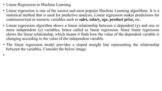
  • 1. • Linear Regression in Machine Learning • Linear regression is one of the easiest and most popular Machine Learning algorithms. It is a statistical method that is used for predictive analysis. Linear regression makes predictions for continuous/real or numeric variables such as sales, salary, age, product price, etc. • Linear regression algorithm shows a linear relationship between a dependent (y) and one or more independent (y) variables, hence called as linear regression. Since linear regression shows the linear relationship, which means it finds how the value of the dependent variable is changing according to the value of the independent variable. • The linear regression model provides a sloped straight line representing the relationship between the variables. Consider the below image: •
  • 2.
  • 3. • Mathematically, we can represent a linear regression as: • y= a0+a1x+ ε • Here, • Y= Dependent Variable (Target Variable) X= Independent Variable (predictor Variable) a0= intercept of the line (Gives an additional degree of freedom) a1 = Linear regression coefficient (scale factor to each input value). ε = random error • The values for x and y variables are training datasets for Linear Regression model representation. • Types of Linear Regression • Linear regression can be further divided into two types of the algorithm: • Simple Linear Regression: If a single independent variable is used to predict the value of a numerical dependent variable, then such a Linear Regression algorithm is called Simple Linear Regression. • Multiple Linear regression: If more than one independent variable is used to predict the value of a numerical dependent variable, then such a Linear Regression algorithm is called Multiple Linear Regression.
  • 4. • Linear Regression Line • A linear line showing the relationship between the dependent and independent variables is called a regression line. A regression line can show two types of relationship: • Positive Linear Relationship: If the dependent variable increases on the Y-axis and independent variable increases on X-axis, then such a relationship is termed as a Positive linear relationship.
  • 5. • Negative Linear Relationship: If the dependent variable decreases on the Y-axis and independent variable increases on the X- axis, then such a relationship is called a negative linear relationship.
  • 6. • Finding the best fit line: • When working with linear regression, our main goal is to find the best fit line that means the error between predicted values and actual values should be minimized. The best fit line will have the least error. • The different values for weights or the coefficient of lines (a0, a1) gives a different line of regression, so we need to calculate the best values for a0 and a1 to find the best fit line, so to calculate this we use cost function. • Cost function- • The different values for weights or coefficient of lines (a0, a1) gives the different line of regression, and the cost function is used to estimate the values of the coefficient for the best fit line. • Cost function optimizes the regression coefficients or weights. It measures how a linear regression model is performing. • We can use the cost function to find the accuracy of the mapping function, which maps the input variable to the output variable. This mapping function is also known as Hypothesis function.
  • 7. • For Linear Regression, we use the Mean Squared Error (MSE) cost function, which is the average of squared error occurred between the predicted values and actual values. It can be written as: • For the above linear equation, MSE can be calculated as: N=Total number of observation Yi = Actual value (a1xi+a0)= Predicted value. Residuals: The distance between the actual value and predicted values is called residual. If the observed points are far from the regression line, then the residual will be high, and so cost function will high. If the scatter points are close to the regression line, then the residual will be small and hence the cost function.
  • 8. • Gradient Descent: • Gradient descent is used to minimize the MSE by calculating the gradient of the cost function. • A regression model uses gradient descent to update the coefficients of the line by reducing the cost function. • It is done by a random selection of values of coefficient and then iteratively update the values to reach the minimum cost function. • Model Performance: • The Goodness of fit determines how the line of regression fits the set of observations. The process of finding the best model out of various models is called optimization. It can be achieved by below method:
  • 9. • R-squared method: • R-squared is a statistical method that determines the goodness of fit. • It measures the strength of the relationship between the dependent and independent variables on a scale of 0-100%. • The high value of R-square determines the less difference between the predicted values and actual values and hence represents a good model. • It is also called a coefficient of determination, or coefficient of multiple determination for multiple regression. • It can be calculated from the below formula:
  • 10. • Assumptions of Linear Regression • Below are some important assumptions of Linear Regression. These are some formal checks while building a Linear Regression model, which ensures to get the best possible result from the given dataset. • Linear relationship between the features and target: Linear regression assumes the linear relationship between the dependent and independent variables. • Small or no multicollinearity between the features: Multicollinearity means high-correlation between the independent variables. Due to multicollinearity, it may difficult to find the true relationship between the predictors and target variables. Or we can say, it is difficult to determine which predictor variable is affecting the target variable and which is not. So, the model assumes either little or no multicollinearity between the features or independent variables.
  • 11. • Homoscedasticity Assumption: Homoscedasticity is a situation when the error term is the same for all the values of independent variables. With homoscedasticity, there should be no clear pattern distribution of data in the scatter plot. • Normal distribution of error terms: Linear regression assumes that the error term should follow the normal distribution pattern. If error terms are not normally distributed, then confidence intervals will become either too wide or too narrow, which may cause difficulties in finding coefficients. It can be checked using the q-q plot. If the plot shows a straight line without any deviation, which means the error is normally distributed. • No autocorrelations: The linear regression model assumes no autocorrelation in error terms. If there will be any correlation in the error term, then it will drastically reduce the accuracy of the model. Autocorrelation usually occurs if there is a dependency between residual errors.
  • 12. • Simple Linear Regression in Machine Learning • Simple Linear Regression is a type of Regression algorithms that models the relationship between a dependent variable and a single independent variable. The relationship shown by a Simple Linear Regression model is linear or a sloped straight line, hence it is called Simple Linear Regression. • The key point in Simple Linear Regression is that the dependent variable must be a continuous/real value. However, the independent variable can be measured on continuous or categorical values. • Simple Linear regression algorithm has mainly two objectives: • Model the relationship between the two variables. Such as the relationship between Income and expenditure, experience and Salary, etc. • Forecasting new observations. Such as Weather forecasting according to temperature, Revenue of a company according to the investments in a year, etc.
  • 13. • Simple Linear Regression Model: • The Simple Linear Regression model can be represented using the below equation: • y= a0+a1x+ ε • Where, • a0= It is the intercept of the Regression line (can be obtained putting x=0) a1= It is the slope of the regression line, which tells whether the line is increasing or decreasing. ε = The error term. (For a good model it will be negligible)
  • 14. • Implementation of Simple Linear Regression Algorithm using Python • Problem Statement example for Simple Linear Regression: • Here we are taking a dataset that has two variables: salary (dependent variable) and experience (Independent variable). The goals of this problem is: • We want to find out if there is any correlation between these two variables • We will find the best fit line for the dataset. • How the dependent variable is changing by changing the independent variable. • In this section, we will create a Simple Linear Regression model to find out the best fitting line for representing the relationship between these two variables. • To implement the Simple Linear regression model in machine learning using Python, we need to follow the below steps:
  • 15. • Step-1: Data Pre-processing • The first step for creating the Simple Linear Regression model is data pre-processing. We have already done it earlier in this tutorial. But there will be some changes, which are given in the below steps: • First, we will import the three important libraries, which will help us for loading the dataset, plotting the graphs, and creating the Simple Linear Regression model. • import numpy as nm • import matplotlib.pyplot as mtp • import pandas as pd • Next, we will load the dataset into our code: • data_set= pd.read_csv('Salary_Data.csv')
  • 16. • By executing the above line of code (ctrl+ENTER), we can read the dataset on our Spyder IDE screen by clicking on the variable explorer option.
  • 17. • The above output shows the dataset, which has two variables: Salary and Experience. • Note: In Spyder IDE, the folder containing the code file must be saved as a working directory, and the dataset or csv file should be in the same folder. • After that, we need to extract the dependent and independent variables from the given dataset. The independent variable is years of experience, and the dependent variable is salary. Below is code for it: • x= data_set.iloc[:, :-1].values • y= data_set.iloc[:, 1].values • In the above lines of code, for x variable, we have taken -1 value since we want to remove the last column from the dataset. For y variable, we have taken 1 value as a parameter, since we want to extract the second column and indexing starts from the zero. • By executing the above line of code, we will get the output for X and Y variable as:
  • 18.
  • 19. • In the above output image, we can see the X (independent) variable and Y (dependent) variable has been extracted from the given dataset. • Next, we will split both variables into the test set and training set. We have 30 observations, so we will take 20 observations for the training set and 10 observations for the test set. We are splitting our dataset so that we can train our model using a training dataset and then test the model using a test dataset. The code for this is given below: • # Splitting the dataset into training and test set. • from sklearn.model_selection import train_test_split • x_train, x_test, y_train, y_test= train_test_split(x, y, test_size= 1/3, random_stat e=0)
  • 20. • By executing the above code, we will get x-test, x-train and y-test, y-train dataset. Consider the below images: • Test-dataset:
  • 22. • For simple linear Regression, we will not use Feature Scaling. Because Python libraries take care of it for some cases, so we don't need to perform it here. Now, our dataset is well prepared to work on it and we are going to start building a Simple Linear Regression model for the given problem. • Step-2: Fitting the Simple Linear Regression to the Training Set: • Now the second step is to fit our model to the training dataset. To do so, we will import the LinearRegression class of the linear_model library from the scikit learn. After importing the class, we are going to create an object of the class named as a regressor. The code for this is given below: 1.#Fitting the Simple Linear Regression model to the training dataset 2.from sklearn.linear_model import LinearRegression 3.regressor= LinearRegression() 4.regressor.fit(x_train, y_train)
  • 23. • In the above code, we have used a fit() method to fit our Simple Linear Regression object to the training set. In the fit() function, we have passed the x_train and y_train, which is our training dataset for the dependent and an independent variable. We have fitted our regressor object to the training set so that the model can easily learn the correlations between the predictor and target variables. After executing the above lines of code, we will get the below output. • Output: • Out[7]: LinearRegression(copy_X=True, fit_intercept=True, n_jobs=None, normalize=False)
  • 24. • Step: 3. Prediction of test set result: • dependent (salary) and an independent variable (Experience). So, now, our model is ready to predict the output for the new observations. In this step, we will provide the test dataset (new observations) to the model to check whether it can predict the correct output or not. • We will create a prediction vector y_pred, and x_pred, which will contain predictions of test dataset, and prediction of training set respectively. • #Prediction of Test and Training set result • y_pred= regressor.predict(x_test) • x_pred= regressor.predict(x_train) • On executing the above lines of code, two variables named y_pred and x_pred will generate in the variable explorer options that contain salary predictions for the training set and test set.
  • 25. • You can check the variable by clicking on the variable explorer option in the IDE, and also compare the result by comparing values from y_pred and y_test. By comparing these values, we can check how good our model is performing. • Step: 4. visualizing the Training set results: • Now in this step, we will visualize the training set result. To do so, we will use the scatter() function of the pyplot library, which we have already imported in the pre-processing step. The scatter () function will create a scatter plot of observations. • In the x-axis, we will plot the Years of Experience of employees and on the y- axis, salary of employees. In the function, we will pass the real values of training set, which means a year of experience x_train, training set of Salaries y_train, and color of the observations. Here we are taking a green color for the observation, but it can be any color as per the choice.
  • 26. • Now, we need to plot the regression line, so for this, we will use the plot() function of the pyplot library. In this function, we will pass the years of experience for training set, predicted salary for training set x_pred, and color of the line. • Next, we will give the title for the plot. So here, we will use the title() function of the pyplot library and pass the name ("Salary vs Experience (Training Dataset)". • After that, we will assign labels for x-axis and y-axis using xlabel() and ylabel() function. • Finally, we will represent all above things in a graph using show(). The code is given below: • mtp.scatter(x_train, y_train, color="green") • mtp.plot(x_train, x_pred, color="red") • mtp.title("Salary vs Experience (Training Dataset)") • mtp.xlabel("Years of Experience") • mtp.ylabel("Salary(In Rupees)") • mtp.show()
  • 27. • Output: • By executing the above lines of code, we will get the below graph plot as an output. •
  • 28. • In the above plot, we can see the real values observations in green dots and predicted values are covered by the red regression line. The regression line shows a correlation between the dependent and independent variable. • The good fit of the line can be observed by calculating the difference between actual values and predicted values. But as we can see in the above plot, most of the observations are close to the regression line, hence our model is good for the training set. • Step: 5. visualizing the Test set results: • In the previous step, we have visualized the performance of our model on the training set. Now, we will do the same for the Test set. The complete code will remain the same as the above code, except in this, we will use x_test, and y_test instead of x_train and y_train. • Here we are also changing the color of observations and regression line to differentiate between the two plots, but it is optional.
  • 29. • #visualizing the Test set results • mtp.scatter(x_test, y_test, color="blue") • mtp.plot(x_train, x_pred, color="red") • mtp.title("Salary vs Experience (Test Dataset)") • mtp.xlabel("Years of Experience") • mtp.ylabel("Salary(In Rupees)") • mtp.show() • Output: • By executing the above line of code, we will get the output as: •
  • 30.
  • 31. • In the above plot, there are observations given by the blue color, and prediction is given by the red regression line. As we can see, most of the observations are close to the regression line, hence we can say our Simple Linear Regression is a good model and able to make good predictions.
  • 32. •Multiple Linear Regression • In the previous topic, we have learned about Simple Linear Regression, where a single Independent/Predictor(X) variable is used to model the response variable (Y). But there may be various cases in which the response variable is affected by more than one predictor variable; for such cases, the Multiple Linear Regression algorithm is used. • Moreover, Multiple Linear Regression is an extension of Simple Linear regression as it takes more than one predictor variable to predict the response variable. We can define it as: • Multiple Linear Regression is one of the important regression algorithms which models the linear relationship between a single dependent continuous variable and more than one independent variable. • Example: • Prediction of CO2 emission based on engine size and number of cylinders in a car.
  • 33. • Some key points about MLR: • For MLR, the dependent or target variable(Y) must be the continuous/real, but the predictor or independent variable may be of continuous or categorical form. • Each feature variable must model the linear relationship with the dependent variable. • MLR tries to fit a regression line through a multidimensional space of data- points. • MLR equation: • In Multiple Linear Regression, the target variable(Y) is a linear combination of multiple predictor variables x1, x2, x3, ...,xn. Since it is an enhancement of Simple Linear Regression, so the same is applied for the multiple linear regression equation, the equation becomes:
  • 34. • Y= b<sub>0</sub>+b<sub>1</sub>x<sub>1</sub>+ b<sub>2</sub>x<sub>2</s ub>+ b<sub>3</sub>x<sub>3</sub>+...... bnxn …….. (a) • Where, • Y= Output/Response variable • b0, b1, b2, b3 , bn....= Coefficients of the model. • x1, x2, x3, x4,...= Various Independent/feature variable • Assumptions for Multiple Linear Regression: • A linear relationship should exist between the Target and predictor variables. • The regression residuals must be normally distributed. • MLR assumes little or no multicollinearity (correlation between the independent variable) in data.
  • 35. • Implementation of Multiple Linear Regression model using Python: • To implement MLR using Python, we have below problem: • Problem Description: • We have a dataset of 50 start-up companies. This dataset contains five main information: R&D Spend, Administration Spend, Marketing Spend, State, and Profit for a financial year. Our goal is to create a model that can easily determine which company has a maximum profit, and which is the most affecting factor for the profit of a company. • Since we need to find the Profit, so it is the dependent variable, and the other four variables are independent variables. Below are the main steps of deploying the MLR model: • Data Pre-processing Steps • Fitting the MLR model to the training set • Predicting the result of the test set
  • 36. • Step-1: Data Pre-processing Step: • The very first step is data pre-processing, which we have already discussed in this tutorial. This process contains the below steps: • Importing libraries: Firstly we will import the library which will help in building the model. Below is the code for it: • # importing libraries • import numpy as nm • import matplotlib.pyplot as mtp • import pandas as pd • Importing dataset: Now we will import the dataset(50_CompList), which contains all the variables. Below is the code for it: • #importing datasets • data_set= pd.read_csv('50_CompList.csv')
  • 37. • Output: We will get the dataset as:
  • 38. • In above output, we can clearly see that there are five variables, in which four variables are continuous and one is categorical variable. • Extracting dependent and independent Variables: • #Extracting Independent and dependent Variable • x= data_set.iloc[:, :-1].values • y= data_set.iloc[:, 4].values • Output: • Out[5]:
  • 39. • rray([[165349.2, 136897.8, 471784.1, 'New York'], • [162597.7, 151377.59, 443898.53, 'California'], • [153441.51, 101145.55, 407934.54, 'Florida'], • [144372.41, 118671.85, 383199.62, 'New York'], • [142107.34, 91391.77, 366168.42, 'Florida'], • [131876.9, 99814.71, 362861.36, 'New York'], • [134615.46, 147198.87, 127716.82, 'California'], • [130298.13, 145530.06, 323876.68, 'Florida'], • [120542.52, 148718.95, 311613.29, 'New York'], • [123334.88, 108679.17, 304981.62, 'California'], • [101913.08, 110594.11, 229160.95, 'Florida'], • [100671.96, 91790.61, 249744.55, 'California'], • [93863.75, 127320.38, 249839.44, 'Florida'], • [91992.39, 135495.07, 252664.93, 'California'], • [119943.24, 156547.42, 256512.92, 'Florida'],
  • 40. • [114523.61, 122616.84, 261776.23, 'New York'], • [78013.11, 121597.55, 264346.06, 'California'], • [94657.16, 145077.58, 282574.31, 'New York'], • [91749.16, 114175.79, 294919.57, 'Florida'], • [86419.7, 153514.11, 0.0, 'New York'], • [76253.86, 113867.3, 298664.47, 'California'], • [78389.47, 153773.43, 299737.29, 'New York'], • [73994.56, 122782.75, 303319.26, 'Florida'], • [67532.53, 105751.03, 304768.73, 'Florida'], • [77044.01, 99281.34, 140574.81, 'New York'], • [64664.71, 139553.16, 137962.62, 'California'], • [75328.87, 144135.98, 134050.07, 'Florida'], • [72107.6, 127864.55, 353183.81, 'New York'], • [66051.52, 182645.56, 118148.2, 'Florida'], • [65605.48, 153032.06, 107138.38, 'New York'], • [61994.48, 115641.28, 91131.24, 'Florida'], • [61136.38, 152701.92, 88218.23, 'New York'], • [63408.86, 129219.61, 46085.25, 'California'], • [55493.95, 103057.49, 214634.81, 'Florida'], • [46426.07, 157693.92, 210797.67, 'California'], • [46014.02, 85047.44, 205517.64, 'New York'], • [28663.76, 127056.21, 201126.82, 'Florida'], • [44069.95, 51283.14, 197029.42, 'California'], • [20229.59, 65947.93, 185265.1, 'New York'],
  • 41. • [38558.51, 82982.09, 174999.3, 'California'], • [28754.33, 118546.05, 172795.67, 'California'], • [27892.92, 84710.77, 164470.71, 'Florida'], • [23640.93, 96189.63, 148001.11, 'California'], • [15505.73, 127382.3, 35534.17, 'New York'], • [22177.74, 154806.14, 28334.72, 'California'], • [1000.23, 124153.04, 1903.93, 'New York'], • [1315.46, 115816.21, 297114.46, 'Florida'], • [0.0, 135426.92, 0.0, 'California'], • [542.05, 51743.15, 0.0, 'New York'], • [0.0, 116983.8, 45173.06, 'California']], dtype=object)
  • 42. • As we can see in the above output, the last column contains categorical variables which are not suitable to apply directly for fitting the model. So we need to encode this variable. • Encoding Dummy Variables: • As we have one categorical variable (State), which cannot be directly applied to the model, so we will encode it. To encode the categorical variable into numbers, we will use the LabelEncoder class. But it is not sufficient because it still has some relational order, which may create a wrong model. So in order to remove this problem, we will use OneHotEncoder, which will create the dummy variables. Below is code for it:
  • 43. • #Catgorical data • from sklearn.preprocessing import LabelEncoder, OneHotEncoder • labelencoder_x= LabelEncoder() • x[:, 3]= labelencoder_x.fit_transform(x[:,3]) • onehotencoder= OneHotEncoder(categorical_features= [3]) • x= onehotencoder.fit_transform(x).toarray() • Here we are only encoding one independent variable, which is state as other variables are continuous.
  • 44.
  • 45. • As we can see in the above output, the state column has been converted into dummy variables (0 and 1). Here each dummy variable column is corresponding to the one State. We can check by comparing it with the original dataset. The first column corresponds to the California State, the second column corresponds to the Florida State, and the third column corresponds to the New York State. • Note: We should not use all the dummy variables at the same time, so it must be 1 less than the total number of dummy variables, else it will create a dummy variable trap. • Now, we are writing a single line of code just to avoid the dummy variable trap: • #avoiding the dummy variable trap: • x = x[:, 1:] • If we do not remove the first dummy variable, then it may introduce multicollinearity in the model.
  • 46.
  • 47. • As we can see in the above output image, the first column has been removed. • Now we will split the dataset into training and test set. The code for this is given below: • # Splitting the dataset into training and test set. • from sklearn.model_selection import train_test_split • x_train, x_test, y_train, y_test= train_test_split(x, y, test_size= 0.2, random_stat e=0) • The above code will split our dataset into a training set and test set. • Output: The above code will split the dataset into training set and test set. You can check the output by clicking on the variable explorer option given in Spyder IDE. The test set and training set will look like the below image:
  • 50. • Note: In MLR, we will not do feature scaling as it is taken care by the library, so we don't need to do it manually. • Step: 2- Fitting our MLR model to the Training set: • Now, we have well prepared our dataset in order to provide training, which means we will fit our regression model to the training set. It will be similar to as we did in Simple Linear Regression model. The code for this will be: • #Fitting the MLR model to the training set: • from sklearn.linear_model import LinearRegression • regressor= LinearRegression() • regressor.fit(x_train, y_train)
  • 51. • Out[9]: LinearRegression(copy_X=True, fit_intercept=True, n_jobs=None, normalize=False) • Now, we have successfully trained our model using the training dataset. In the next step, we will test the performance of the model using the test dataset. • Step: 3- Prediction of Test set results: • The last step for our model is checking the performance of the model. We will do it by predicting the test set result. For prediction, we will create a y_pred vector. Below is the code for it: • #Predicting the Test set result; • y_pred= regressor.predict(x_test) • By executing the above lines of code, a new vector will be generated under the variable explorer option. We can test our model by comparing the predicted values and test set values. • Output:
  • 52.
  • 53. • In the above output, we have predicted result set and test set. We can check model performance by comparing these two value index by index. For example, the first index has a predicted value of 103015$ profit and test/real value of 103282$ profit. The difference is only of 267$, which is a good prediction, so, finally, our model is completed here. • We can also check the score for training dataset and test dataset. Below is the code for it: • print('Train Score: ', regressor.score(x_train, y_train)) • print('Test Score: ', regressor.score(x_test, y_test)) • Output: The score is: • Train Score: 0.9501847627493607 • Test Score: 0.9347068473282446
  • 54. • The above score tells that our model is 95% accurate with the training dataset and 93% accurate with the test dataset. • Note: In the next topic, we will see how we can improve the performance of the model using the Backward Elimination process. • Applications of Multiple Linear Regression: • There are mainly two applications of Multiple Linear Regression: • Effectiveness of Independent variable on prediction: • Predicting the impact of changes:
  • 55. • What is Backward Elimination? • Backward elimination is a feature selection technique while building a machine learning model. It is used to remove those features that do not have a significant effect on the dependent variable or prediction of output. There are various ways to build a model in Machine Learning, which are: • All-in • Backward Elimination • Forward Selection • Bidirectional Elimination • Score Comparison • Above are the possible methods for building the model in Machine learning, but we will only use here the Backward Elimination process as it is the fastest method.
  • 56. • Steps of Backward Elimination • Below are some main steps which are used to apply backward elimination process: • Step-1: Firstly, We need to select a significance level to stay in the model. (SL=0.05) • Step-2: Fit the complete model with all possible predictors/independent variables. • Step-3: Choose the predictor which has the highest P-value, such that. • If P-value >SL, go to step 4. • Else Finish, and Our model is ready. • Step-4: Remove that predictor. • Step-5: Rebuild and fit the model with the remaining variables.
  • 57. • Need for Backward Elimination: An optimal Multiple Linear Regression model: • In the previous chapter, we discussed and successfully created our Multiple Linear Regression model, where we took 4 independent variables (R&D spend, Administration spend, Marketing spend, and state (dummy variables)) and one dependent variable (Profit). But that model is not optimal, as we have included all the independent variables and do not know which independent model is most affecting and which one is the least affecting for the prediction. • Unnecessary features increase the complexity of the model. Hence it is good to have only the most significant features and keep our model simple to get the better result. • So, in order to optimize the performance of the model, we will use the Backward Elimination method. This process is used to optimize the performance of the MLR model as it will only include the most affecting feature and remove the least affecting feature. Let's start to apply it to our MLR model.
  • 58. • Steps for Backward Elimination method: • We will use the same model which we build in the previous chapter of MLR. Below is the complete code for it:
  • 59. • # importing libraries • import numpy as nm • import matplotlib.pyplot as mtp • import pandas as pd • • #importing datasets • data_set= pd.read_csv('50_CompList.csv') • • #Extracting Independent and dependent Variable • x= data_set.iloc[:, :-1].values • y= data_set.iloc[:, 4].values • • #Catgorical data • from sklearn.preprocessing import LabelEncoder, OneHotEncoder • labelencoder_x= LabelEncoder() • x[:, 3]= labelencoder_x.fit_transform(x[:,3]) • onehotencoder= OneHotEncoder(categorical_features= [3]) • x= onehotencoder.fit_transform(x).toarray()
  • 60. • #Avoiding the dummy variable trap: • x = x[:, 1:] • # Splitting the dataset into training and test set. • from sklearn.model_selection import train_test_split • x_train, x_test, y_train, y_test= train_test_split(x, y, test_size= 0.2, random_sta te=0) • #Fitting the MLR model to the training set: • from sklearn.linear_model import LinearRegression • regressor= LinearRegression() • regressor.fit(x_train, y_train) •
  • 61. • #Predicting the Test set result; • y_pred= regressor.predict(x_test) • #Checking the score • print('Train Score: ', regressor.score(x_train, y_train)) • print('Test Score: ', regressor.score(x_test, y_test)) • From the above code, we got training and test set result as: • Train Score: 0.9501847627493607 • Test Score: 0.9347068473282446 • The difference between both scores is 0.0154. • Note: On the basis of this score, we will estimate the effect of features on our model after using the Backward elimination process. •
  • 62. • Step: 1- Preparation of Backward Elimination: • Importing the library: Firstly, we need to import the statsmodels.formula.api library, which is used for the estimation of various statistical models such as OLS(Ordinary Least Square). Below is the code for it: • import statsmodels.api as smf • Adding a column in matrix of features: As we can check in our MLR equation (a), there is one constant term b0, but this term is not present in our matrix of features, so we need to add it manually. We will add a column having values x0 = 1 associated with the constant term b0. To add this, we will use append function of Numpy library (nm which we have already imported into our code), and will assign a value of 1. Below is the code for it. • x = nm.append(arr = nm.ones((50,1)).astype(int), values=x, axis=1)
  • 63. • Here we have used axis =1, as we wanted to add a column. For adding a row, we can use axis =0. • Output: By executing the above line of code, a new column will be added into our matrix of features, which will have all values equal to 1. We can check it by clicking on the x dataset under the variable explorer option.
  • 64.
  • 65. • As we can see in the above output image, the first column is added successfully, which corresponds to the constant term of the MLR equation. • Step: 2: • Now, we are actually going to apply a backward elimination process. Firstly we will create a new feature vector x_opt, which will only contain a set of independent features that are significantly affecting the dependent variable. • Next, as per the Backward Elimination process, we need to choose a significant level(0.5), and then need to fit the model with all possible predictors. So for fitting the model, we will create a regressor_OLS object of new class OLS of statsmodels library. Then we will fit it by using the fit() method. • Next we need p-value to compare with SL value, so for this we will use summary() method to get the summary table of all the values. Below is the code for it:
  • 66. • x_opt=x [:, [0,1,2,3,4,5]] • regressor_OLS=sm.OLS(endog = y, exog=x_opt).fit() • regressor_OLS.summary() • Output: By executing the above lines of code, we will get a summary table. Consider the below image:
  • 67.
  • 68. • In the above image, we can clearly see the p-values of all the variables. Here x1, x2 are dummy variables, x3 is R&D spend, x4 is Administration spend, and x5 is Marketing spend. • From the table, we will choose the highest p-value, which is for x1=0.953 Now, we have the highest p-value which is greater than the SL value, so will remove the x1 variable (dummy variable) from the table and will refit the model. Below is the code for it: • x_opt=x[:, [0,2,3,4,5]] • regressor_OLS=sm.OLS(endog = y, exog=x_opt).fit() • regressor_OLS.summary() • Output:
  • 69.
  • 70. • As we can see in the output image, now five variables remain. In these variables, the highest p-value is 0.961. So we will remove it in the next iteration. • Now the next highest value is 0.961 for x1 variable, which is another dummy variable. So we will remove it and refit the model. Below is the code for it: • x_opt= x[:, [0,3,4,5]] • regressor_OLS=sm.OLS(endog = y, exog=x_opt).fit() • regressor_OLS.summary() • Output:
  • 71.
  • 72. • In the above output image, we can see the dummy variable(x2) has been removed. And the next highest value is .602, which is still greater than .5, so we need to remove it. • Now we will remove the Admin spend which is having .602 p-value and again refit the model. • x_opt=x[:, [0,3,5]] • regressor_OLS=sm.OLS(endog = y, exog=x_opt).fit() • regressor_OLS.summary() • Output:
  • 73.
  • 74. • As we can see in the above output image, the variable (Admin spend) has been removed. But still, there is one variable left, which is marketing spend as it has a high p-value (0.60). So we need to remove it. • Finally, we will remove one more variable, which has .60 p-value for marketing spend, which is more than a significant level. Below is the code for it: • x_opt=x[:, [0,3]] • regressor_OLS=sm.OLS(endog = y, exog=x_opt).fit() • regressor_OLS.summary() • Output:
  • 75.
  • 76. • As we can see in the above output image, only two variables are left. So only the R&D independent variable is a significant variable for the prediction. So we can now predict efficiently using this variable. • Estimating the performance: • In the previous topic, we have calculated the train and test score of the model when we have used all the features variables. Now we will check the score with only one feature variable (R&D spend). Our dataset now looks like:
  • 77.
  • 78. • Below is the code for Building Multiple Linear Regression model by only using R&D spend: • # importing libraries • import numpy as nm • import matplotlib.pyplot as mtp • import pandas as pd • • #importing datasets • data_set= pd.read_csv('50_CompList1.csv') • • #Extracting Independent and dependent Variable • x_BE= data_set.iloc[:, :-1].values • y_BE= data_set.iloc[:, 1].values • • • # Splitting the dataset into training and test set. • from sklearn.model_selection import train_test_split • x_BE_train, x_BE_test, y_BE_train, y_BE_test= train_test_split(x_BE, y_BE, test_size= 0.2, random_s tate=0)
  • 79. • #Fitting the MLR model to the training set: • from sklearn.linear_model import LinearRegression • regressor= LinearRegression() • regressor.fit(nm.array(x_BE_train).reshape(-1,1), y_BE_train) • • #Predicting the Test set result; • y_pred= regressor.predict(x_BE_test) • • #Cheking the score • print('Train Score: ', regressor.score(x_BE_train, y_BE_train)) • print('Test Score: ', regressor.score(x_BE_test, y_BE_test))
  • 80. • Output: • After executing the above code, we will get the Training and test scores as: • Train Score: 0.9449589778363044 • Test Score: 0.9464587607787219 • As we can see, the training score is 94% accurate, and the test score is also 94% accurate. The difference between both scores is .00149. This score is very much close to the previous score, i.e., 0.0154, where we have included all the variables. • We got this result by using one independent variable (R&D spend) only instead of four variables. Hence, now, our model is simple and accurate.
  • 81. • ML Polynomial Regression • Polynomial Regression is a regression algorithm that models the relationship between a dependent(y) and independent variable(x) as nth degree polynomial. The Polynomial Regression equation is given below: y= b0+b1x1+ b2x1 2+ b2x1 3+...... bnx1 n •It is also called the special case of Multiple Linear Regression in ML. Because we add some polynomial terms to the Multiple Linear regression equation to convert it into Polynomial Regression. •It is a linear model with some modification in order to increase the accuracy. •The dataset used in Polynomial regression for training is of non-linear nature. •It makes use of a linear regression model to fit the complicated and non-linear functions and datasets. •Hence, "In Polynomial regression, the original features are converted into Polynomial features of required degree (2,3,..,n) and then modeled using a linear model."
  • 82. Need for Polynomial Regression: The need of Polynomial Regression in ML can be understood in the below points: •If we apply a linear model on a linear dataset, then it provides us a good result as we have seen in Simple Linear Regression, but if we apply the same model without any modification on a non-linear dataset, then it will produce a drastic output. Due to which loss function will increase, the error rate will be high, and accuracy will be decreased. •So for such cases, where data points are arranged in a non-linear fashion, we need the Polynomial Regression model. We can understand it in a better way using the below comparison diagram of the linear dataset and non-linear dataset.
  • 83. • In the above image, we have taken a dataset which is arranged non-linearly. So if we try to cover it with a linear model, then we can clearly see that it hardly covers any data point. On the other hand, a curve is suitable to cover most of the data points, which is of the Polynomial model. • Hence, if the datasets are arranged in a non-linear fashion, then we should use the Polynomial Regression model instead of Simple Linear Regression. • Note: A Polynomial Regression algorithm is also called Polynomial Linear Regression because it does not depend on the variables, instead, it depends on the coefficients, which are arranged in a linear fashion. • Equation of the Polynomial Regression Model: Simple Linear Regression equation: y = b0+b1x .........(a) Multiple Linear Regression equation: y= b0+b1x+ b2x2+ b3x3+....+ bnxn .........(b) Polynomial Regression equation: y= b0+b1x + b2x2+ b3x3+....+ bnxn ..........(c)
  • 84. • When we compare the above three equations, we can clearly see that all three equations are Polynomial equations but differ by the degree of variables. The Simple and Multiple Linear equations are also Polynomial equations with a single degree, and the Polynomial regression equation is Linear equation with the nth degree. So if we add a degree to our linear equations, then it will be converted into Polynomial Linear equations. • Note: To better understand Polynomial Regression, you must have knowledge of Simple Linear Regression.
  • 85. • Implementation of Polynomial Regression using Python: • Here we will implement the Polynomial Regression using Python. We will understand it by comparing Polynomial Regression model with the Simple Linear Regression model. So first, let's understand the problem for which we are going to build the model. • Problem Description: There is a Human Resource company, which is going to hire a new candidate. The candidate has told his previous salary 160K per annum, and the HR have to check whether he is telling the truth or bluff. So to identify this, they only have a dataset of his previous company in which the salaries of the top 10 positions are mentioned with their levels. By checking the dataset available, we have found that there is a non-linear relationship between the Position levels and the salaries. Our goal is to build a Bluffing detector regression model, so HR can hire an honest candidate. Below are the steps to build such a model.
  • 86.
  • 87. • Steps for Polynomial Regression: • The main steps involved in Polynomial Regression are given below: • Data Pre-processing • Build a Linear Regression model and fit it to the dataset • Build a Polynomial Regression model and fit it to the dataset • Visualize the result for Linear Regression and Polynomial Regression model. • Predicting the output. • Note: Here, we will build the Linear regression model as well as Polynomial Regression to see the results between the predictions. And Linear regression model is for reference.
  • 88. • Data Pre-processing Step: • The data pre-processing step will remain the same as in previous regression models, except for some changes. In the Polynomial Regression model, we will not use feature scaling, and also we will not split our dataset into training and test set. It has two reasons: • The dataset contains very less information which is not suitable to divide it into a test and training set, else our model will not be able to find the correlations between the salaries and levels. • In this model, we want very accurate predictions for salary, so the model should have enough information. • The code for pre-processing step is given below:
  • 89. • # importing libraries • import numpy as nm • import matplotlib.pyplot as mtp • import pandas as pd • • #importing datasets • data_set= pd.read_csv('Position_Salaries.csv') • • #Extracting Independent and dependent Variable • x= data_set.iloc[:, 1:2].values • y= data_set.iloc[:, 2].values
  • 90. • Explanation: • In the above lines of code, we have imported the important Python libraries to import dataset and operate on it. • Next, we have imported the dataset 'Position_Salaries.csv', which contains three columns (Position, Levels, and Salary), but we will consider only two columns (Salary and Levels). • After that, we have extracted the dependent(Y) and independent variable(X) from the dataset. For x-variable, we have taken parameters as [:,1:2], because we want 1 index(levels), and included :2 to make it as a matrix. • Output: • By executing the above code, we can read our dataset as:
  • 91.
  • 92. • As we can see in the above output, there are three columns present (Positions, Levels, and Salaries). But we are only considering two columns because Positions are equivalent to the levels or may be seen as the encoded form of Positions. • Here we will predict the output for level 6.5 because the candidate has 4+ years' experience as a regional manager, so he must be somewhere between levels 7 and 6. • Building the Linear regression model: • Now, we will build and fit the Linear regression model to the dataset. In building polynomial regression, we will take the Linear regression model as reference and compare both the results. The code is given below: • #Fitting the Linear Regression to the dataset • from sklearn.linear_model import LinearRegression • lin_regs= LinearRegression() • lin_regs.fit(x,y)
  • 93. • In the above code, we have created the Simple Linear model using lin_regs object of LinearRegression class and fitted it to the dataset variables (x and y). • Output: • Out[5]: LinearRegression(copy_X=True, fit_intercept=True, n_jobs=None, normalize=False) • Building the Polynomial regression model: • Now we will build the Polynomial Regression model, but it will be a little different from the Simple Linear model. Because here we will use PolynomialFeatures class of preprocessing library. We are using this class to add some extra features to our dataset.
  • 94. • #Fitting the Polynomial regression to the dataset • from sklearn.preprocessing import PolynomialFeatures • poly_regs= PolynomialFeatures(degree= 2) • x_poly= poly_regs.fit_transform(x) • lin_reg_2 =LinearRegression() • lin_reg_2.fit(x_poly, y) • In the above lines of code, we have used poly_regs.fit_transform(x), because first we are converting our feature matrix into polynomial feature matrix, and then fitting it to the Polynomial regression model. The parameter value(degree= 2) depends on our choice. We can choose it according to our Polynomial features. • After executing the code, we will get another matrix x_poly, which can be seen under the variable explorer option:
  • 95.
  • 96. • Next, we have used another LinearRegression object, namely lin_reg_2, to fit our x_poly vector to the linear model. • Output • Out[11]: LinearRegression(copy_X=True, fit_intercept=True, n_jobs=None, normalize=False) • Visualizing the result for Linear regression: • Now we will visualize the result for Linear regression model as we did in Simple Linear Regression. Below is the code for it: • #Visulaizing the result for Linear Regression model • mtp.scatter(x,y,color="blue") • mtp.plot(x,lin_regs.predict(x), color="red") • mtp.title("Bluff detection model(Linear Regression)") • mtp.xlabel("Position Levels") • mtp.ylabel("Salary") • mtp.show()
  • 97. • Output: In the above output image, we can clearly see that the regression line is so far from the datasets. Predictions are in a red straight line, and blue points are actual values. If we consider this output to predict the value of CEO, it will give a salary of approx. 600000$, which is far away from the real value. So we need a curved model to fit the dataset other than a straight line.
  • 98. • Visualizing the result for Polynomial Regression • Here we will visualize the result of Polynomial regression model, code for which is little different from the above model. • Code for this is given below: • #Visulaizing the result for Polynomial Regression • mtp.scatter(x,y,color="blue") • mtp.plot(x, lin_reg_2.predict(poly_regs.fit_transform(x)), color="red") • mtp.title("Bluff detection model(Polynomial Regression)") • mtp.xlabel("Position Levels") • mtp.ylabel("Salary") • mtp.show()
  • 99. • In the above code, we have taken lin_reg_2.predict(poly_regs.fit_transform(x), instead of x_poly, because we want a Linear regressor object to predict the polynomial features matrix. • Output
  • 100. • As we can see in the above output image, the predictions are close to the real values. The above plot will vary as we will change the degree. • For degree= 3: • If we change the degree=3, then we will give a more accurate plot, as shown in the below image. •
  • 101. • SO as we can see here in the above output image, the predicted salary for level 6.5 is near to 170K$-190k$, which seems that future employee is saying the truth about his salary. • Degree= 4: Let's again change the degree to 4, and now will get the most accurate plot. Hence we can get more accurate results by increasing the degree of Polynomial
  • 102. • Predicting the final result with the Linear Regression model: • Now, we will predict the final output using the Linear regression model to see whether an employee is saying truth or bluff. So, for this, we will use the predict() method and will pass the value 6.5. Below is the code for it: • lin_pred = lin_regs.predict([[6.5]]) • print(lin_pred) • [330378.78787879] • Predicting the final result with the Polynomial Regression model: • Now, we will predict the final output using the Polynomial Regression model to compare with Linear model. Below is the code for it:
  • 103. • poly_pred = lin_reg_2.predict(poly_regs.fit_transform([[6.5]])) • print(poly_pred) • [158862.45265153] • As we can see, the predicted output for the Polynomial Regression is [158862.45265153], which is much closer to real value hence, we can say that future employee is saying true.