Mip formulations quick_reference (2)

www.ﬁco.com Make every decision countTM
FICOTM
Xpress Optimization Suite
MIP formulations and
linearizations
Quick reference
Last update 29 June, 2009

Published by Fair Isaac Corporation
c Copyright Fair Isaac Corporation 2009. All rights reserved.
All trademarks referenced in this manual that are not the property of Fair Isaac are acknowledged.
All companies, products, names and data contained within this book are completely fictitious and are used solely to illustrate
the use of Xpress. Any similarity between these names or data and reality is purely coincidental.
How to Contact the Xpress Team
Information, Sales and Licensing
USA, CANADA AND ALL AMERICAS
Email: XpressSalesUS@fico.com
WORLDWIDE
Email: XpressSalesUK@fico.com
Tel: +44 1926 315862
Fax: +44 1926 315854
FICO, Xpress team
Leam House, 64 Trinity Street
Leamington Spa
Warwickshire CV32 5YN
UK
Product Support
Email: Support@fico.com
(Please include ’Xpress’ in the subject line)
Telephone:
NORTH AMERICA
Tel (toll free): +1 (877) 4FI-SUPP
Fax: +1 (402) 496-2224
EUROPE, MIDDLE EAST, AFRICA
Tel: +44 (0) 870-420-3777
UK (toll free): 0800-0152-153
South Africa (toll free): 0800-996-153
Fax: +44 (0) 870-420-3778
ASIA-PACIFIC, LATIN AMERICA, CARIBBEAN
Tel: +1 (415) 446-6185
Brazil (toll free): 0800-891-6146
For the latest news and Xpress software and documentation updates, please visit the Xpress website at
http://www.fico.com/xpress or subscribe to our mailing list.

MIP formulations
FICOTM
Xpress Optimization Suite
MIP formulations and linearizations
Quick reference
29 June, 2009
Contents
1 Introduction . . . . . . . . . . . . . . . . . . . . . . . . . . . . . . . . . . . . . . . . . . . 1
1.1 Integer Programming entities supported in Xpress . . . . . . . . . . . . . . . . . 1
1.2 Integer Programming entities in Mosel . . . . . . . . . . . . . . . . . . . . . . . 2
1.3 Integer Programming entities in BCL . . . . . . . . . . . . . . . . . . . . . . . . . 3
2 Binary variables . . . . . . . . . . . . . . . . . . . . . . . . . . . . . . . . . . . . . . . . . 4
2.1 Logical conditions . . . . . . . . . . . . . . . . . . . . . . . . . . . . . . . . . . . . 4
2.2 Minimum values . . . . . . . . . . . . . . . . . . . . . . . . . . . . . . . . . . . . . 4
2.3 Maximum values . . . . . . . . . . . . . . . . . . . . . . . . . . . . . . . . . . . . 5
2.4 Absolute values . . . . . . . . . . . . . . . . . . . . . . . . . . . . . . . . . . . . . 5
2.5 Logical AND . . . . . . . . . . . . . . . . . . . . . . . . . . . . . . . . . . . . . . . 6
2.6 Logical OR . . . . . . . . . . . . . . . . . . . . . . . . . . . . . . . . . . . . . . . . 6
2.7 Logical NOT . . . . . . . . . . . . . . . . . . . . . . . . . . . . . . . . . . . . . . . 7
2.8 Product values . . . . . . . . . . . . . . . . . . . . . . . . . . . . . . . . . . . . . . 7
2.9 Disjunctions . . . . . . . . . . . . . . . . . . . . . . . . . . . . . . . . . . . . . . . 7
2.10 Minimum activity level . . . . . . . . . . . . . . . . . . . . . . . . . . . . . . . . . 8
3 MIP formulations using other entities . . . . . . . . . . . . . . . . . . . . . . . . . . . . 8
3.1 Batch sizes . . . . . . . . . . . . . . . . . . . . . . . . . . . . . . . . . . . . . . . . 9
3.2 Ordered alternatives . . . . . . . . . . . . . . . . . . . . . . . . . . . . . . . . . . 9
3.3 Price breaks . . . . . . . . . . . . . . . . . . . . . . . . . . . . . . . . . . . . . . . 10
3.4 Non-linear functions . . . . . . . . . . . . . . . . . . . . . . . . . . . . . . . . . . 12
3.5 Minimum activity level . . . . . . . . . . . . . . . . . . . . . . . . . . . . . . . . . 15
3.6 Partial integer variables . . . . . . . . . . . . . . . . . . . . . . . . . . . . . . . . 16
4 Indicator constraints . . . . . . . . . . . . . . . . . . . . . . . . . . . . . . . . . . . . . . 16
4.1 Inverse implication . . . . . . . . . . . . . . . . . . . . . . . . . . . . . . . . . . . 17
4.2 Logic constructs . . . . . . . . . . . . . . . . . . . . . . . . . . . . . . . . . . . . . 18
1 Introduction
This quick reference guide presents a collection of MIP model formulations for Xpress-Optimizer,
including standard linearization techniques involving binary variables, the use of more speciﬁc
modeling objects such as SOS and partial integer variables, and reformulations of logic
constraints through indicator constraints.
1.1 Integer Programming entities supported in Xpress
• Binary variables (BV) – decision variables that must take either the value 0 or the value 1,
sometimes called 0/1 variables;
Introduction c 2009 Fair Isaac Corporation. All rights reserved. page 1

MIP formulations
• Integer variables (UI) – decision variables that must take on integer values. Some upper limit
must be specified;
• Partial integer variables (PI) – decision variables that must take integer values below a
specified limit but can take any value above that limit;
• Semi-continuous variables (SC) – decision variables that must take on either the value 0, or
any value in a range whose lower an upper limits are specified. SCs help model situations
where, if a variable is to be used at all, it has to be at some minimum level;
• Semi-continuous integer variables (SI) – decision variables that must take either the value 0,
or any integer value in a range whose lower and upper limits are specified;
• Special ordered sets of type one (SOS1) – an ordered set of variables of which at most one
can take a nonzero value;
• Special ordered sets of type two (SOS2) – an ordered set of variables of which at most two
can be nonzero, and if two are nonzero, they must be consecutive in their ordering.
Remarks
• The solution values of binary and integer variables are real valued, not integer valued.
• At an optimal MIP solution, the actual values of the binary and integer variables will be
integer – to within a certain tolerance.
1.2 Integer Programming entities in Mosel
Definition: integer programming types are defined as unary constraints on previously declared
decision variables of type mpvar; name the constraints if you want to be able to access/modify
them.
declarations
d: mpvar
ifmake: array(PRODS,LINES) of mpvar
x: mpvar
end-declarations
d is_binary ! Single binary variable
forall(p in PRODS, l in LINES)
ifmake(p,l) is_binary ! An array of binaries
ACtr:= x is_integer ! An integer variable
x >= MINVAL ! Lower bound on the variable
x <= MAXVAL ! Upper bound on the variable
! MINVAL,MAXVAL: values between -MAX_REAL and MAX_REAL
...
ACtr:= x is_partint 10 ! Change type to partial integer
...
ACtr:= 0 ! Delete constraint
! Equivalently:
ACtr:= x is_continuous ! Change type to continuous
Solving: with Xpress-Optimizer (Mosel module mmxprs) any problem containing integer
programming entities is automatically solved as a MIP problem, to solve just the LP relaxation use
option XPRS_TOP (if following up with MIP search) or XPRS_LIN (ignore all MIP information) for
maximize / minimize.
Accessing the solution: for obtaining solution values of decision variables and linear expressions
use getsol (alternative syntax: .sol); the MIP problem status is returned by the function
getparam("XPRS_MIPSTATUS")

MIP formulations
case getparam("XPRS_MIPSTATUS") of
XPRS_MIP_NOT_LOADED,
XPRS_MIP_LP_NOT_OPTIMAL: writeln("Solving not started")
XPRS_MIP_LP_OPTIMAL: writeln("LP unbounded or infeasible")
XPRS_MIP_NO_SOL_FOUND,
XPRS_MIP_INFEAS: writeln("MIP search started, no solution")
XPRS_MIP_SOLUTION,
XPRS_MIP_OPTIMAL: writeln("MIP solution: ", , getobjval)
end-case
writeln("x: ", getsol(x))
writeln("d: ", d.sol)
1.3 Integer Programming entities in BCL
The BCL code extracts in this document are formulated for the BCL C++ interface. The other BCL
interfaces (C, Java, C#, VB) work similarly, please refer to the Xpress documentation for further
detail.
Deﬁnition: Integer Programming types are speciﬁed when creating decision variables (type
XPRBvar); types may be changed with setType.
XPRBprob prob("test");
XPRBvar d, ifmake[NP][NL], x;
int p,l;
d = prob.newVar("d", XPRB_BV); // Single binary variable
for (p = 0; p < NP; p++) // An array of binaries
for (l = 0; l < NL; l++)
ifmake[p][l] = prob.newVar("ifmake", XPRB_BV);
x = prob.newVar("x", XPRB_UI, MINVAL, MAXVAL); // An integer variable
// MINVAL,MAXVAL: reals between -XPRB_INFINITY and XPRB_INFINITY
...
x.setType(XPRB_PI); // Change type to partial integer
x.setLim(10);
...
x.setType(XPRB_PL); // Change type to continuous
Solving: use option "g" in solve / minim / maxim to solve a problem as a MIP problem (per
default only the LP relaxation is solved).
prob.minim("g");
Accessing the solution: for obtaining solution values of decision variables and linear expressions
use getSol; the MIP problem status is returned by getMIPstatus.
int mipstatus = prob.getMIPStat();
switch (mipstatus) {
case XPRB_MIP_NOT_LOADED:
case XPRB_MIP_LP_NOT_OPTIMAL:
cout << "Solving not started" << endl;
break;
case XPRB_MIP_LP_OPTIMAL:
cout << "LP unbounded or infeasible" << endl;
break;
case XPRB_MIP_NO_SOL_FOUND:
case XPRB_MIP_INFEAS:
cout << "MIP search started, no solution" << endl;
break;
case XPRB_MIP_SOLUTION:

MIP formulations
case XPRB_MIP_OPTIMAL:
cout << "MIP solution: " << prob.getObjVal() << endl;
break;
}
cout << x.getName() << ": " << x.getSol() << endl;
2 Binary variables
Binary decision variables
• take value 0 or 1
• model a discrete decision
– yes/no
– on/off
– open/close
– build or don’t build
– strategy A or strategy B
2.1 Logical conditions
Projects A, B, C, D, ... with associated binary variables a, b, c, d, ... which are 1 if we decide to do
the project and 0 if we decide not to do the project.
At most N of A, B, C,... a + b + c+. . . ≤ N
At least N of A, B, C,... a + b + c+. . . ≥ N
Exactly N of A, B, C,... a + b + c+. . . = N
If A then B b ≥ a
Not B ¯b = 1 − b
If A then not B a + b ≤ 1
If not A then B a + b ≥ 1
If A then B, and if B then A a = b
If A then B and C; A only if B and C b ≥ a and c ≥ a
or alternatively: a ≤ (b + c) / 2
If A then B or C b + c ≥ a
If B or C then A a ≥ b and a ≥ c
or alternatively: a ≥ 1
2 · (b + c)
If B and C then A a ≥ b + c − 1
If two or more of B, C, D or E then A a ≥ 1
3 · (b + c + d + e − 1)
If M or more of N projects (B, C, D, ...) then A a ≥ b+c+d+...−M+1
N−M+1
2.2 Minimum values
y = min{x1, x2} for two continuous variables x1, x2
• Must know lower and upper bounds
Binary variables c 2009 Fair Isaac Corporation. All rights reserved. page 4

MIP formulations
L1 ≤ x1 ≤ U1 [1.1]
L2 ≤ x2 ≤ U2 [1.2]
• Introduce binary variables d1, d2 to mean
di 1 if xi is the minimum value;
0 otherwise
• MIP formulation:
y ≤ x1 [2.1]
y ≤ x2 [2.2]
y ≥ x1 − (U1 − Lmin)(1 − d1) [3.1]
y ≥ x2 − (U2 − Lmin)(1 − d2) [3.2]
d1 + d2 = 1 [4]
• Generalization to y = min{x1, x2, . . . , xn}
Li ≤ xi ≤ Ui [1.i]
y ≤ xi [2.i]
y ≥ xi − (Ui − Lmin)(1 − di) [3.i]
i di = 1 [4]
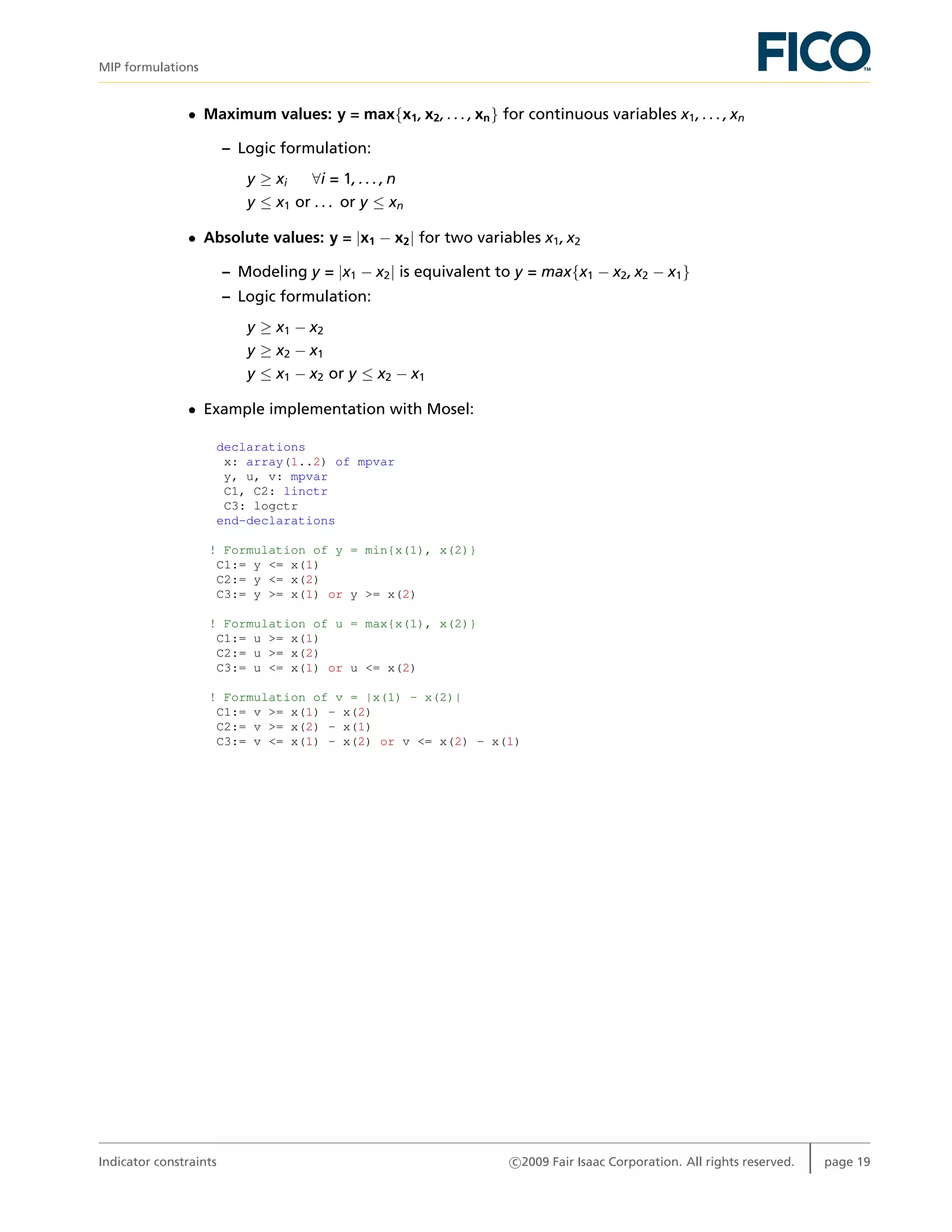
2.3 Maximum values
y = max{x1, x2, . . . , xn} for continuous variables x1, . . . , xn
Li ≤ xi ≤ Ui [1.i]
• Introduce binary variables d1, . . . , dn
di = 1 if xi is the minimum value, 0 otherwise
• MIP formulation
Li ≤ xi ≤ Ui [1.i]
y ≥ xi [2.i]
y ≤ xi + (Umax − Li)(1 − di) [3.i]
i di = 1 [4]
2.4 Absolute values
y = |x1 − x2| for two variables x1, x2 with 0 ≤ xi ≤ U
• Introduce binary variables d1, d2 to mean
d1 : 1 if x1 − x2 is the positive value
d2 : 1 if x2 − x1 is the positive value

MIP formulations
• MIP formulation
0 ≤ xi ≤ U [1.i]
0 ≤ y − (x1 − x2) ≤ 2 · U · d2 [2]
0 ≤ y − (x2 − x1) ≤ 2 · U · d1 [3]
d1 + d2 = 1 [4]
2.5 Logical AND
d = min{d1, d2} for two binary variables d1, d2, or equivalently
d = d1 · d2 (see Section 2.8), or
d = d1 AND d2 as a logical expression
• IP formulation
d ≤ d1 [1.1]
d ≤ d2 [1.2]
d ≥ d1 + d2 − 1 [2]
d ≥ 0 [3]
• Generalization to d = min{d1, d2, . . . , dn}
d ≤ di [1.i]
d ≥ i di − (n − 1) [2]
d ≥ 0 [3]
Note: equivalent to d = d1 · d2·. . . ·dn
and (as a logical expression): d = d1 AND d2 AND ... AND dn
2.6 Logical OR
d = max{d1, d2} for two binary variables d1, d2, or
d = d1 OR d2 as a logical expression
• IP formulation
d ≥ d1 [1.1]
d ≥ d2 [1.2]
d ≤ d1 + d2 [2]
d ≤ 1 [3]
• Generalization to d = max{d1, d2, . . . , dn}
d ≥ di [1.i]
d ≤ i di [2.i]
d ≤ 1 [3]
Note: equivalent to d = d1 OR d2. . . OR dn

MIP formulations
2.7 Logical NOT
d = NOT d1 for one binary variable d1
• IP formulation
d = 1 − d1
2.8 Product values
y = x · d for one continuous variable x, one binary variable d
L ≤ x ≤ U
Ld ≤ y ≤ Ud [1]
L(1 − d) ≤ x − y ≤ U(1 − d) [2]
Product of two binaries: d3 = d1 · d2
d3 ≤ d1
d3 ≤ d2
d3 ≥ d1 + d2 − 1
2.9 Disjunctions
Either 5 ≤ x ≤ 10 or 80 ≤ x ≤ 100
• Introduce a new binary variable:
ifupper: 0 if 5 ≤ x ≤ 10; 1 if 80 ≤ x ≤ 100
x ≤ 10 + (100 − 10) · ifupper [1]
x ≥ 5 + (80 − 5) · ifupper [2]
• Generalization to Either L1 ≤ i Aixi ≤ U1 or L2 ≤ i Aixi ≤ U2 (with U1 ≤ L2)
i Aixi ≤ U1 + (U2 − U1) · ifupper [1]
i Aixi ≥ L1 + (L2 − L1) · ifupper [2]

MIP formulations
2.10 Minimum activity level
Continuous production rate make that may be 0 (the plant is not operating) or between allowed
production limits MAKEMIN and MAKEMAX
• Introduce a binary variable ifmake to mean
ifmake : 0 if plant is shut
1 plant is open
MIP formulation:
make ≥ MAKEMIN · ifmake [1]
make ≤ MAKEMAX · ifmake [2]
Note: see Section 3.5 for an alternative formulation using semi-continuous variables
• The ifmake binary variable also allows us to model ﬁxed costs
– FCOST: ﬁxed production cost
– VCOST: variable production cost
MIP formulation:
cost = FCOST · ifmake + VCOST · make [3]
make ≥ MAKEMIN · ifmake [1]
make ≤ MAKEMAX · ifmake [2]
3 MIP formulations using other entities
In principle, all you need in building MIP models are continuous variables and binary variables.
But it is convenient to extend the set of modeling entities to embrace objects that frequently
occur in practice.
Integer decision variables
• values 0, 1, 2, ... up to small upper bound
• model discrete quantities
• try to use partial integer variables instead of integer variables with a very large upper bound
Semi-continuous variable
• may be zero, or any value between the intermediate bound and the upper bound
• Semi-continuous integer variables also available: may be zero, or any integer value between
the intermediate bound and the upper bound
Special ordered sets
• set of decision variables
MIP formulations using other entities c 2009 Fair Isaac Corporation. All rights reserved. page 8

MIP formulations
• each variable has a different ordering value, which orders the set
• Special ordered sets of type 1 (SOS1): at most one variable may be non-zero
• Special ordered sets of type 2 (SOS2): at most two variables may be non-zero; the non-zero
variables must be adjacent in ordering
3.1 Batch sizes
Must deliver in batches of 10, 20, 30, ...
• Decision variables
nship number of batches delivered: integer
ship quantity delivered: continuous
• Constraint formulation
ship = 10 · nship
3.2 Ordered alternatives
Suppose you have N possible investments of which at most one can be selected. The capital cost is
CAPi and the expected return is RETi.
• Often use binary variables to choose between alternatives. However, SOS1 are more
efficient to choose between a set of graded (ordered) alternatives.
• Define a variable di to represent the decision, di = 1 if investment i is picked
• Binary variable (standard) formulation
di : binary variables
Maximize: ret = i RETidi
i di ≤ 1
i CAPidi ≤ MAXCAP
• SOS1 formulation
{di; ordering value CAPi} : SOS1
Maximize: ret = i RETidi
i di ≤ 1
i CAPidi ≤ MAXCAP
• Special ordered sets in Mosel
– special ordered sets are a special type of linear constraint
– the set includes all variables in the constraint
– the coefficient of a variable is used as the ordering value (i.e., each value must be
unique)

MIP formulations
declarations
I=1..4
d: array(I) of mpvar
CAP: array(I) of real
My_Set, Ref_row: linctr
end-declarations
My_Set:= sum(i in I) CAP(i)*d(i) is_sos1
or alternatively (must be used if a coefficient is 0):
Ref_row:= sum(i in I) CAP(i)*d(i)
makesos1(My_Set, union(i in I) d(i), Ref_row)
• Special ordered sets in BCL
– a special ordered set is an object of type XPRBsos
– the set includes all variables from the specified linear expression or constraint that have
a coefficient different from 0
– the coefficient of a variable is used as the ordering value (i.e., each value must be
unique)
XPRBprob prob("testsos");
XPRBvar d[I];
XPRBexpr le;
XPRBsos My_Set;
double CAP[I];
int i;
for(i=0; i<I; i++) d[i] = prob.newVar("d");
for(i=0; i<I; i++) le += CAP[i]*d[i];
My_Set = prob.newSos("My_Set", XPRB_S1, le);
3.3 Price breaks
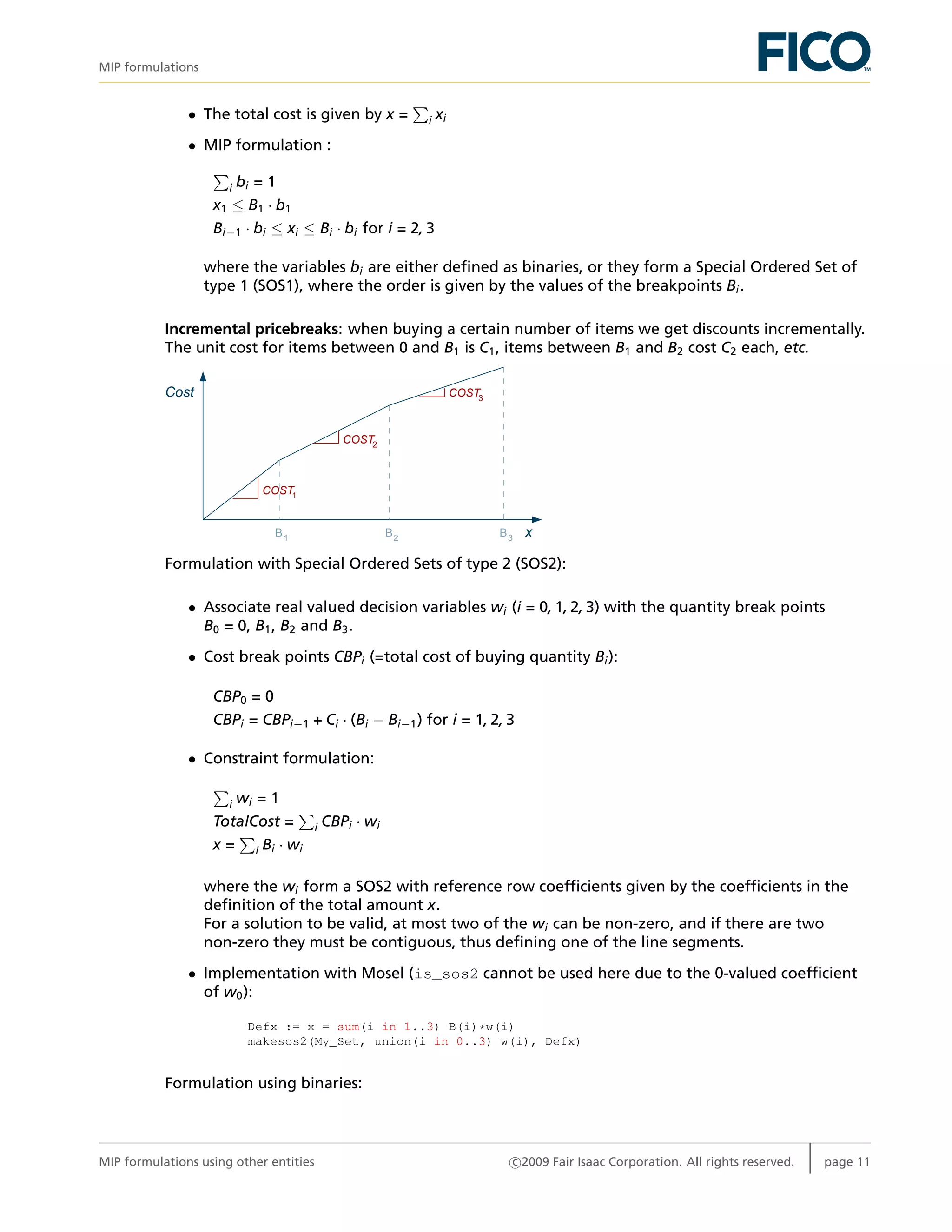
All items discount: when buying a certain number of items we get discounts on all items that we
buy if the quantity we buy lies in certain price bands.
Cost
xB1 B2 B3
COST1
COST2
COST3
less than B1 COST1 each
≥ B1 and < B2 COST2 each
≥ B2 and < B3 COST3 each
• Define binary variables bi (i=1,2,3), where bi is 1 if we pay a unit cost of COSTi.
• Real decision variables xi represent the number of items bought at price COSTi.

MIP formulations
• The total cost is given by x = i xi
• MIP formulation :
i bi = 1
x1 ≤ B1 · b1
Bi−1 · bi ≤ xi ≤ Bi · bi for i = 2, 3
where the variables bi are either defined as binaries, or they form a Special Ordered Set of
type 1 (SOS1), where the order is given by the values of the breakpoints Bi.
Incremental pricebreaks: when buying a certain number of items we get discounts incrementally.
The unit cost for items between 0 and B1 is C1, items between B1 and B2 cost C2 each, etc.
Cost
xB3B2B1
COST1
COST
COST3
2
Formulation with Special Ordered Sets of type 2 (SOS2):
• Associate real valued decision variables wi (i = 0, 1, 2, 3) with the quantity break points
B0 = 0, B1, B2 and B3.
• Cost break points CBPi (=total cost of buying quantity Bi):
CBP0 = 0
CBPi = CBPi−1 + Ci · (Bi − Bi−1) for i = 1, 2, 3
• Constraint formulation:
i wi = 1
TotalCost = i CBPi · wi
x = i Bi · wi
where the wi form a SOS2 with reference row coefficients given by the coefficients in the
definition of the total amount x.
For a solution to be valid, at most two of the wi can be non-zero, and if there are two
non-zero they must be contiguous, thus defining one of the line segments.
• Implementation with Mosel (is_sos2 cannot be used here due to the 0-valued coefficient
of w0):
Defx := x = sum(i in 1..3) B(i)*w(i)
makesos2(My_Set, union(i in 0..3) w(i), Defx)
Formulation using binaries:

MIP formulations
• Define binary variables bi (i=1,2,3), where bi is 1 if we have bought any items at a unit cost
of COSTi.
• Real decision variables xi (i=1,..3) for the number of items bought at price COSTi.
• Total amount bought: x = i xi
• Constraint formulation:
(Bi − Bi−1) · bi+1 ≤ xi ≤ (Bi − Bi−1) · bi for i = 1, 2
x3 ≤ (B3 − B2) · b3
b1 ≥ b2 ≥ b3
3.4 Non-linear functions
Can model non-linear functions in the same way as incremental pricebreaks
• approximate the non-linear function with a piecewise linear function
• use an SOS2 to model the piecewise linear function
Non-linear function in a single variable
y
xR(1) R(2) R(3) R(4)
F(1)
F(4)
F(3)
F(2)
1
2
3
4
• x-coordinates of the points: R1, ..., R4
y-coordinates F1, ..., F4. So point 1 is (R1, F1) etc.
• Let weights (decision variables) associated with point i be wi (i=1,...,4)
• Form convex combinations of the points using weights wi to get a combination point (x,y):
x = i wi · Ri
y = i wi · Fi
i wi = 1
where the variables wi form an SOS2 set with ordering coefficients defined by values Ri.

MIP formulations
• Mosel implementation:
declarations
I=1..4
x,y: mpvar
w: array(I) of mpvar
R,F: array(I) of real
end-declarations
! ...assign values to arrays R and F...
! Define the SOS-2 with "reference row" coefficients from R
Defx:= sum(i in I) R(i)*w(i) is_sos2
sum(i in I) w(i) = 1
! The variable and the corresponding function value we want to approximate
x = Defx
y = sum(i in I) F(i)*w(i)
• BCL implementation:
XPRBvar x, y, w[I];
XPRBexpr Defx, le, ly;
double R[I], F[I];
int i;
// ...assign values to arrays R and F...
// Create the decision variables
x = prob.newVar("x"); y = prob.newVar("y");
for(i=0; i<I; i++) w[i] = prob.newVar("w");
// Define the SOS-2 with "reference row" coefficients from R
for(i=0; i<I; i++) Defx += R[i]*w[i];
prob.newSos("Defx", XPRB_S2, Defx);
for(i=0; i<I; i++) le += w[i];
prob.newCtr("One", le == 1);
// The variable and the corresponding function value we want to approximate
prob.newCtr("Eqx", x == Defx);
for(i=0; i<I; i++) ly += F[i]*w[i];
prob.newCtr("Eqy", y == ly);
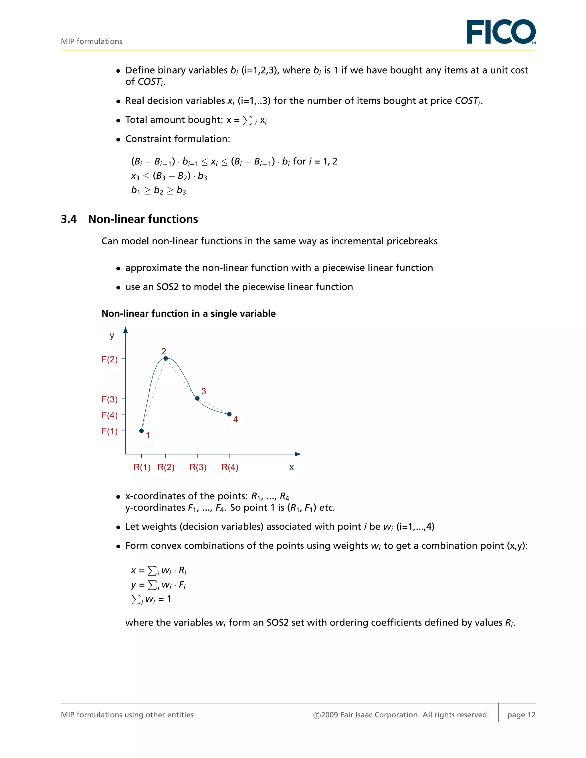
Non-linear function in two variables
Interpolation of a function f in two variables: approximate f at a point P by the corners C of the
enclosing square of a rectangular grid (NB: the representation of P=(x,y) by the four points C
obviously means a fair amount of degeneracy).
P
C
C C
C
1 7 8 965432
1
2
4
5
6
3

MIP formulations
• x-coordinates of grid points: X1, ..., Xn
y-coordinates of grid points: Y1, ..., Ym. So grid points are (Xi, Yj).
• Function evaluation at grid points: FXY11, ..., FXYnm
• Define weights (decision variables) associated with x and y coordinates, wxi respectively wyj,
and for each grid point (X(i), Y(j)) define a variable wxyij
• Form convex combinations of the points using the weights to get a combination point (x,y)
and the corresponding function approximation:
x = i wxi · Xi
y = j wyj · Yj
f = ij wxyij · FXYij
∀i = 1, . . . , n : j wxyij = wxi
∀j = 1, . . . , m : i wxyij = wyj
i wxi = 1
j wyj = 1
where the variables wxi form an SOS2 set with ordering coefficients defined by values Xi,
and the variables wyj are a second SOS2 set with coordinate values Yj as ordering
coefficients.
• Mosel implementation:
declarations
RX,RY:range
X: array(RX) of real ! x coordinate values of grid points
Y: array(RY) of real ! y coordinate values of grid points
FXY: array(RX,RY) of real ! Function evaluation at grid points
end-declarations
! ... initialize data
declarations
wx: array(RX) of mpvar ! Weight on x coordinate
wy: array(RY) of mpvar ! Weight on y coordinate
wxy: array(RX,RY) of mpvar ! Weight on (x,y) coordinates
x,y,f: mpvar
end-declarations
! Definition of SOS (assuming coordinate values <>0)
sum(i in RX) X(i)*wx(i) is_sos2
sum(j in RY) Y(j)*wy(j) is_sos2
! Constraints
forall(i in RX) sum(j in RY) wxy(i,j) = wx(i)
forall(j in RY) sum(i in RX) wxy(i,j) = wy(j)
sum(i in RX) wx(i) = 1
sum(j in RY) wy(j) = 1
! Then x, y and f can be calculated using
x = sum(i in RX) X(i)*wx(i)
y = sum(j in RY) Y(j)*wy(j)
f = sum(i in RX,j in RY) FXY(i,j)*wxy(i,j)
! f can take negative or positive values (unbounded variable)
f is_free

MIP formulations
• BCL implementation:
XPRBvar x, y, f;
XPRBvar wx[NX], wy[NY], wxy[NX][NY]; // Weights on coordinates
XPRBexpr Defx, Defy, le, lexy, lx, ly;
double DX[NX], DY[NY];
double FXY[NX][NY];
int i,j;
// ... initialize data arrays DX, DY, FXY
x = prob.newVar("x"); y = prob.newVar("y");
f = prob.newVar("f", XPRB_PL, -XPRB_INFINITY, XPRB_INFINITY); // Unbounded variable
for(i=0; i<NX; i++) wx[i] = prob.newVar("wx");
for(j=0; j<NY; j++) wy[j] = prob.newVar("wy");
for(i=0; i<NX; i++)
for(j=0; j<NY; j++) wxy[i][j] = prob.newVar("wxy");
// Definition of SOS
for(i=0; i<NX; i++) Defx += X[i]*wx[i];
prob.newSos("Defx", XPRB_S2, Defx);
for(j=0; j<NY; j++) Defy += Y[j]*wy[j];
prob.newSos("Defy", XPRB_S2, Defy);
// Constraints
for(i=0; i<NX; i++) {
le = 0;
for(j=0; j<NY; j++) le += wxy[i][j];
prob.newCtr("Sumx", le == wx[i]);
}
for(j=0; j<NY; j++) {
le = 0;
for(i=0; i<NX; i++) le += wxy[i][j];
prob.newCtr("Sumy", le == wy[j]);
}
for(i=0; i<NX; i++) lx += wx[i];
prob.newCtr("Convx", lx == 1);
for(j=0; j<NY; j++) ly += wy[j];
prob.newCtr("Convy", ly == 1);
// Calculate x, y and the corresponding function value f we want to approximate
prob.newCtr("Eqx", x == Defx);
prob.newCtr("Eqy", y == Defy);
for(i=0; i<NX; i++)
for(j=0; j<NY; j++) lexy += FXY[i][j]*wxy[i][j];
prob.newCtr("Eqy", f == lexy);
3.5 Minimum activity level
Continuous production rate make. May be 0 (the plant is not operating) or between allowed
production limits MAKEMIN and MAKEMAX
• Can impose using a semi-continuous variable: may be zero, or any value between the
intermediate bound and the upper bound
• Mosel:
make is_semcont MAKEMIN
make <= MAKEMAX

MIP formulations
• BCL:
make = prob.newVar("make", XPRB_SC, 0, MAKEMAX);
make.setLim(MAKEMIN);
• Semi-continuous variables are slightly more efficient than the alternative binary variable
formulation that we saw before. But if you incur fixed costs on any non-zero activity, you
must use the binary variable formulation (see Section 2.10).
3.6 Partial integer variables
• In general, try to keep the upper bound on integer variables as small as possible. This
reduces the number of possible integer values, and so reduces the time to solve the problem.
• Sometimes this is not possible – a variable has a large upper bound and must take integer
values.
⇒ Try to use partial integer variables instead of integer variables with a very large upper
bound: takes integer values for small values, where it is important to be precise, but takes
real values for larger values, where it is OK to round the value afterwards.
• For example, it may be important to clarify whether the value is 0, 1, 2, ..., 10, but above 10
it is OK to get a real value and round it.
• Mosel:
x is_partint 10 ! x is integer valued from 0 to 10
x <= 20 ! x takes real values from 10 to 20
• BCL:
x = prob.newVar("x", XPRB_PI, 0, 20);
x.setLim(10);
4 Indicator constraints
Indicator constraints
• associate a binary variable b with a linear constraint C
• model an implication:
’if b = 1 then C’, in symbols: b → C, or
’if b = 0 then C’, in symbols: ¯b → C
(the constraint C is active only if the condition is true)
• use indicator constraints for the composition of logic expressions
Indicator constraints in Mosel: for the definition of indicator constraints (function indicator of
module mmxprs) you need a binary variable (type mpvar) and a linear inequality constraint (type
linctr). You also have to specify the type of the implication (1 for b → C and -1 for ¯b → C). The
subroutine indicator returns a new constraint of type logctr that can be used in the
composition of other logic expressions (see Section 4.2 below).
Indicator constraints c 2009 Fair Isaac Corporation. All rights reserved. page 16

MIP formulations
uses "mmxprs"
declarations
R=1..10
C: array(range) of linctr
L: array(range) of logctr
x: array(R) of mpvar
b: array(R) of mpvar
end-declarations
forall(i in R) b(i) is_binary ! Variables for indicator constraints
C(2):= x(2)<=5
! Define 2 indicator constraints
L(1):= indicator(1, b(1), x(1)+x(2)>=12) ! b(1)=1 -> x(1)+x(2)>=12
indicator(-1, b(2), C(2)) ! b(2)=0 -> x(2)<=5
C(2):=0 ! Delete auxiliary constraint definition
Indicator constraints in BCL: an indicator constraint is defined by associating a binary decision
variable (XPRBvar) and an integer flag (1 for b → C and -1 for ¯b → C) with a linear inequality or
range constraint (XPRBctr). By defining an indicator constraint (function XPRBsetindicator or
method XPRBctr.setIndicator() depending on the host language) the type of the constraint
itself gets changed; it can be reset to ’standard constraint’ by calling the setIndicator function
with flag value 0.
XPRBprob prob("testind");
XPRBvar x[N], b[N];
XPRBctr IndCtr[N];
int i;
for(i=0;i<N;i++) x[i] = prob.newVar("x", XPRB_PL); // Continuous variables
for(i=0;i<N;i++) b[i] = prob.newVar("b", XPRB_BV); // Indicator variables
// Define 2 linear inequality constraints
IndCtr[0] = prob.newCtr("L1", x[0]+x[1]>=12);
IndCtr[1] = prob.newCtr("L2", x[1]<=5);
// Turn the 2 constraints into indicator constraints
IndCtr[0].setIndicator(1, b[0]); // b(0)=1 -> x(0)+x(1)>=12
IndCtr[1].setIndicator(-1, b[1]); // b(1)=0 -> x(1)<=5
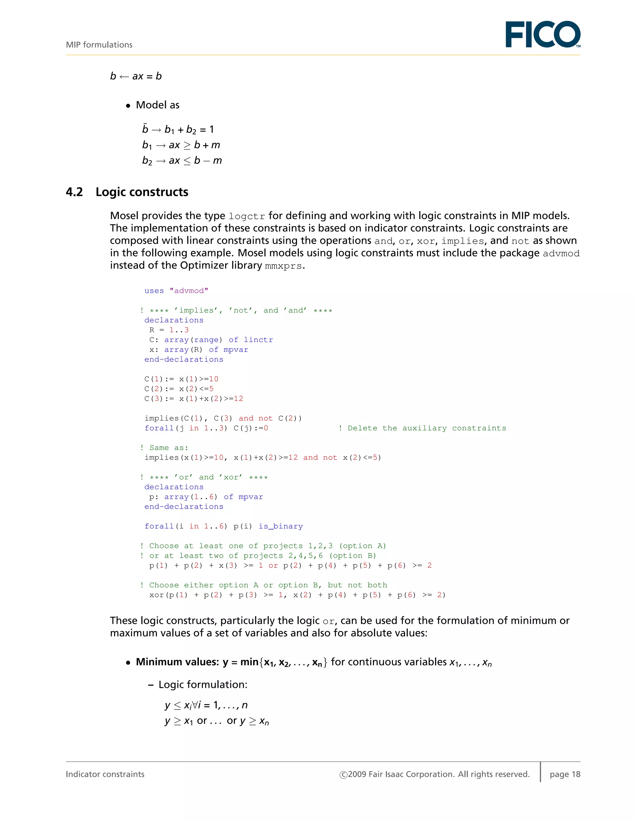
4.1 Inverse implication
b ← ax ≥ b
• Model as
¯b → ax ≤ b − m
where m is a sufficiently small value (slightly larger than the feasibility tolerance)
b ← ax ≤ b
• Model as
¯b → ax ≥ b + m

MIP formulations
b ← ax = b
• Model as
¯b → b1 + b2 = 1
b1 → ax ≥ b + m
b2 → ax ≤ b − m
4.2 Logic constructs
Mosel provides the type logctr for deﬁning and working with logic constraints in MIP models.
The implementation of these constraints is based on indicator constraints. Logic constraints are
composed with linear constraints using the operations and, or, xor, implies, and not as shown
in the following example. Mosel models using logic constraints must include the package advmod
instead of the Optimizer library mmxprs.
uses "advmod"
! **** ’implies’, ’not’, and ’and’ ****
declarations
R = 1..3
C: array(range) of linctr
x: array(R) of mpvar
end-declarations
C(1):= x(1)>=10
C(2):= x(2)<=5
C(3):= x(1)+x(2)>=12
implies(C(1), C(3) and not C(2))
forall(j in 1..3) C(j):=0 ! Delete the auxiliary constraints
! Same as:
implies(x(1)>=10, x(1)+x(2)>=12 and not x(2)<=5)
! **** ’or’ and ’xor’ ****
declarations
p: array(1..6) of mpvar
end-declarations
forall(i in 1..6) p(i) is_binary
! Choose at least one of projects 1,2,3 (option A)
! or at least two of projects 2,4,5,6 (option B)
p(1) + p(2) + x(3) >= 1 or p(2) + p(4) + p(5) + p(6) >= 2
! Choose either option A or option B, but not both
xor(p(1) + p(2) + p(3) >= 1, x(2) + p(4) + p(5) + p(6) >= 2)
These logic constructs, particularly the logic or, can be used for the formulation of minimum or
maximum values of a set of variables and also for absolute values:
• Minimum values: y = min{x1, x2, . . . , xn} for continuous variables x1, . . . , xn
– Logic formulation:
y ≤ xi∀i = 1, . . . , n
y ≥ x1 or . . . or y ≥ xn

MIP formulations
• Maximum values: y = max{x1, x2, . . . , xn} for continuous variables x1, . . . , xn
y ≥ xi ∀i = 1, . . . , n
y ≤ x1 or . . . or y ≤ xn
• Absolute values: y = |x1 − x2| for two variables x1, x2
– Modeling y = |x1 − x2| is equivalent to y = max{x1 − x2, x2 − x1}
y ≥ x1 − x2
y ≥ x2 − x1
y ≤ x1 − x2 or y ≤ x2 − x1
• Example implementation with Mosel:
declarations
x: array(1..2) of mpvar
y, u, v: mpvar
C1, C2: linctr
C3: logctr
end-declarations
! Formulation of y = min{x(1), x(2)}
C1:= y <= x(1)
C2:= y <= x(2)
C3:= y >= x(1) or y >= x(2)
! Formulation of u = max{x(1), x(2)}
C1:= u >= x(1)
C2:= u >= x(2)
C3:= u <= x(1) or u <= x(2)
! Formulation of v = |x(1) - x(2)|
C1:= v >= x(1) - x(2)
C2:= v >= x(2) - x(1)
C3:= v <= x(1) - x(2) or v <= x(2) - x(1)

Mip formulations quick_reference (2)

Recommended

Recommended

More Related Content

Viewers also liked

Viewers also liked (17)

Similar to Mip formulations quick_reference (2)

Similar to Mip formulations quick_reference (2) (20)

Recently uploaded

Recently uploaded (20)

Mip formulations quick_reference (2)