Excel is a spreadsheet program that allows you to store, organize, and analyze information. In this lesson, you will learn your way around the Excel 2010

1. CSE111 Introduction to Computer Applications
Lecture 10
Introduction to MS Excel 2010-Part 2
Prepared by Asst. Prof. Dr. Mohamed KURDI
Revised and presented by Asst. Prof. Dr. Samsun M. BAŞARICI

2. SUMMARY OF THE LAST WEEK
• Exploring & identifying MS Excel user interface elements.
• Moving around worksheets.
• Selecting cells, rows, and columns.
• Editing & formatting worksheets.
• Inserting & deleting rows and columns.
• Deleting rows & columns.
• Changing row heights & column widths.
• Hiding & unhiding rows & columns.
• Selecting worksheets
• Navigating between worksheets
• Renaming worksheets
• Inserting & deleting worksheets
• Moving & copying worksheets
• Switching between MS Excel views
• Freezing & unfreezing panes
• Using templates

3. LEARNİNG OBJECTİVES
Understand and apply the following skills:
• How to enter a formula.
• How to edit a formula.
• How to use parentheses to change the operators precendence.
• How to copy/paste a formula.
• How to choose between the paste options (Paste,Values, Formulas, Formatting, and
Pase Special).
• How to insert a function.
• How to use the count functions (Count, Countif, and Countifs).
• How to use the sum functions (Sum, Sumif, and Sumifs).
• How to use the logical functions (If, And, and Or).
• How to use the statistical functions (Average, Averageif, Median, Mode, Standard
Deviation, Min, Max, Large, and Small).

4. OUTLİNES
 Formulas and Functions
 Entering a Formula
 Editing a Formula
 Changing the Operators Precedence
 Copying/Pasting a Formula
 Paste Options
• Paste
• Values
• Formulas
• Formatting
• Pase Special
 Inserting a Function
 Count Functions (Count, Countif, Countifs)
 Sum Functions (Sum, Sumif, Sumifs)
 Logical Functions (If, And, Or)
 Statistical Functions (Average, Averageif, Median, Mode, Standard Deviation, Min,
Max, Large, and Small).

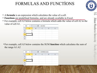
5. FORMULAS AND FUNCTİONS
• A formula is an expression which calculates the value of a cell.
• Functions are predefined formulas, and are already available in Excel.
• For example, cell A3 below contains a formula which adds the value of cell A2 to the
value of cell A1.
•For example, cell A3 below contains the SUM function which calculates the sum of
the range A1:A2

6. ENTERİNG A FORMULA
To enter a formula, execute the following steps.
1. Select a cell.
2. To let Excel know that you want to enter a formula, type an equal sign (=).
3. For example, type the formula A1+A2.
Tip: instead of typing A1 and A2, simply select cell A1 and cell A2.
4. Change the value of cell A1 to 3.
Excel automatically recalculates the value of cell A3. This is one of Excel's most
powerful features!

7. EDİTİNG A FORMULA
When you select a cell, Excel shows the value or formula of the cell in the formula bar.
To edit a formula:
1. click in the formula bar and change the formula.
2. Press Enter

8. OPERATOR PRECEDENCE
Excel uses a default order in which calculations occur. If a part of the formula is in
parentheses, that part will be calculated first. It then performs multiplication or division
calculations. Once this is complete, Excel will add and subtract the remainder of your
formula. See the example below.
First, Excel performs multiplication (A1 * A2). Next, Excel adds the value of cell A3 to this
result.
Another example,
First, Excel calculates the part in parentheses (A2+A3). Next, it multiplies this result by
the value of cell A1.

9. COPYİNG/PASTİNG A FORMULA
When you copy a formula, Excel automatically adjusts
the cell references for each new cell the formula is
copied to. To understand this, execute the following
steps.

10. COPYİNG/PASTİNG A FORMULA
When you copy a formula, Excel automatically adjusts
the cell references for each new cell the formula is
copied to. To understand this, execute the following
steps.
1. Enter the formula shown below into cell A4.

11. COPYİNG/PASTİNG A FORMULA
When you copy a formula, Excel automatically adjusts
the cell references for each new cell the formula is
copied to. To understand this, execute the following
steps.
1. Enter the formula shown below into cell A4.
2. Select cell A4, right click, and then click Copy (or press CTRL + c), and then select cell
B4, right click, and then click Paste under 'Paste Options:' (or press CTRL + v).Or You
can also drag the formula to cell B4. Select cell A4, click on the lower right corner of
cell A4 and drag it across to cell B4. This is much easier and gives the exact same result!

12. COPYİNG/PASTİNG A FORMULA
When you copy a formula, Excel automatically adjusts
the cell references for each new cell the formula is
copied to. To understand this, execute the following
steps.
1. Enter the formula shown below into cell A4.
2. Select cell A4, right click, and then click Copy (or press CTRL + c), and then select cell
B4, right click, and then click Paste under 'Paste Options:' (or press CTRL + v).Or You
can also drag the formula to cell B4. Select cell A4, click on the lower right corner of
cell A4 and drag it across to cell B4. This is much easier and gives the exact same result!
Result. The formula in cell B4 references
the values in column B.

13. PASTE OPTİONS - THE PASTE OPTİON
The Paste option pastes everything.
1. Select cell B5, right click, and then click Copy (or press CTRL + c).
2. Select cell F5, right click, and then click Paste under 'Paste Options:' (or press CTRL + v).
Result

14. PASTE OPTİONS - THE VALUES OPTİON
The Values option pastes the result of the formula.
1. Select cell B5, right click, and then click Copy (or press CTRL + c).
2. Select cell D5, right click, and then click Values under 'Paste Options:'
Result

15. PASTE OPTİONS - THE FORMULAS OPTİON
The Formulas option only pastes the formula.
1. Select cell B5, right click, and then click Copy (or press CTRL + c).
2. Select cell F5, right click, and then click Formulas under 'Paste Options:'
Result

16. PASTE OPTİONS – THE FORMATTİNG OPTİON
The Formatting option only pastes the formatting.
1. Select cell B5, right click, and then click Copy (or press CTRL + c).
2. Select cell D5, right click, and then click Formatting under 'Paste Options:'
Result
Note: the Format Painter copy/pastes formatting even quicker.

17. PASTE OPTİONS – THE PASTE SPECİAL OPTİON
The Paste Special dialog box offers many more paste options. To launch the Paste Special
dialog box, execute the following steps.
1. Select cell B5, right click, and then
click Copy (or press CTRL + c).
2. Next, select cell D5, right click, and then
click Paste Special.

18. PASTE OPTİONS – THE PASTE SPECİAL OPTİON
The Paste Special dialog box offers many more paste options. To launch the Paste Special
dialog box, execute the following steps.
1. Select cell B5, right click, and then
click Copy (or press CTRL + c).
2. Next, select cell D5, right click, and then
click Paste Special.
3. The Paste Special dialog box appears.
4. Choose the option that fits you, then click OK.

19. INSERTİNG A FUNCTİON
To insert a function, execute the following steps.
1. Select a cell.

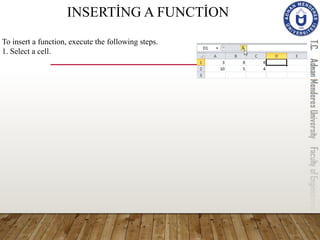
20. INSERTİNG A FUNCTİON
To insert a function, execute the following steps.
1. Select a cell.
2. Click the Insert Function button.

21. INSERTİNG A FUNCTİON
To insert a function, execute the following steps.
1. Select a cell.
2. Click the Insert Function button.
3.The Insert Function dialog box appears, search for a
function or select a function from a category.
For example, choose COUNTIF from the Statistical
category.

22. INSERTİNG A FUNCTİON
To insert a function, execute the following steps.
1. Select a cell.
2. Click the Insert Function button.
3.The Insert Function dialog box appears, search for a
function or select a function from a category.
For example, choose COUNTIF from the Statistical
category.
4. Click OK, the Function Arguments dialog box appears.
5. Click in the Range box and select the range A1:C2.
6. Click in the Criteria box and type >5.

23. INSERTİNG A FUNCTİON
To insert a function, execute the following steps.
1. Select a cell.
2. Click the Insert Function button.
3.The Insert Function dialog box appears, search for a
function or select a function from a category.
For example, choose COUNTIF from the Statistical
category.
4. Click OK, the Function Arguments dialog box appears.
5. Click in the Range box and select the range A1:C2.
6. Click in the Criteria box and type >5.
7. Click OK.
Result. Excel counts the number of cells that
are higher than 5.

24. COUNT FUNCTİONS- THE COUNT FUNCTİON
To count the number of cells that contain numbers, use the following COUNT
function.

25. COUNT FUNCTİONS – THE COUNTIF FUNCTİON
To count cells based on one criteria (for example, higher than 9), use the following
COUNTIF function.
Note: in contrast to the COUNT function, cells can contain text as well.

26. COUNT FUNCTİONS – THE COUNTIFS FUNCTİON
To count cells based on multiple criteria (for example, green and higher than 9), use
the following COUNTIFS function.

27. SUM FUNCTİONS - THE SUM FUNCTİON
To sum a range of cells, use the following SUM function.

28. SUM FUNCTİONS - THE SUMIF FUNCTİON
To sum cells based on one criteria (for example, higher than 9), use the following SUMIF
function (two arguments).

29. To sum cells based on multiple criteria (for example, blue and green), use the following
SUMIFS function (first argument is the range to sum).
SUM FUNCTİONS - THE SUMIFS FUNCTİON

30. The IF Function checks whether a condition is met, and returns one value if TRUE and
another value if FALSE.
Select cell C2 and enter the following function.
LOGİCAL FUNCTİONS - THE IF FUNCTİON
The IF function returns Correct because the value in cell A1 is higher than 10.

31. The AND Function returns TRUE if all conditions are true and returns FALSE if any of
the conditions are false.
Select cell D2 and enter the following formula.
LOGİCAL FUNCTİONS - THE AND FUNCTİON
The AND function returns FALSE because the value in cell B2 is not higher than 5. As a
result the IF function returns Incorrect.

32. The OR Function returns TRUE if any of the conditions are TRUE and returns FALSE
if all conditions are false.
Select cell E2 and enter the following formula.
LOGİCAL FUNCTİONS - THE OR FUNCTİON
The OR function returns TRUE because the value in cell A1 is higher than 10. As a result
the IF function returns Correct.
General note: the AND and OR function can check up to 255 conditions

33. STATİSTİCAL FUNCTİONS – THE AVERAGE FUNCTION
To calculate the average of a range of cells, use the following AVERAGE function.

34. STATİSTİCAL FUNCTİONS – THE AVERAGEIF FUNCTION
To average cells based on one criteria, use the following AVERAGEIF function.
For example, to calculate the average excluding zeros.
Note: <> means not equal to

35. STATİSTİCAL FUNCTİONS – THE MEDIAN FUNCTION
To find the median (or middle number), use the following MEDIAN function.
Check:

36. STATİSTİCAL FUNCTİONS – THE MODE FUNCTION
To find the most frequently occurring number, use the following MODE function

37. STATİSTİCAL FUNCTİONS – THE STEDV FUNCTION
To calculate the standard deviation, use the following STEDV function.

38. STATİSTİCAL FUNCTİONS – THE MIN FUNCTION
To find the minimum value, use the efollowing MIN function.

39. STATİSTİCAL FUNCTİONS – THE MAX FUNCTION
To find the maximum value, use the following MAX function.

40. STATİSTİCAL FUNCTİONS – THE LARGE FUNCTION
To find the third largest number, use the following LARGE function.
Check:

41. STATİSTİCAL FUNCTİONS – THE SMALL FUNCTION
To find the second smallest number, use the following SMALL function
Check:

42. References
All the materials presented in this lecture are copyrighted by
http://www.excel-easy.com