Download to read offline


![6 CHAPTER 1. INTRODUCTION TO PARALLEL PROCESSING
Suppose we wish to multiply an nx1 vector X by an nxn matrix A, putting the product
in an nx1 vector Y, and we have p processors to share the work.
In all the forms of parallelism, each node could be assigned some of the rows of A, and that node
would multiply X by those rows, thus forming part of Y.
Note that in typical applications, the matrix A would be very large, say thousands of rows, pos-
sibly even millions. Otherwise the computation could be done quite satisfactorily in a serial, i.e.
nonparallel manner, making parallel processing unnecessary..
1.3.2 Shared-Memory
1.3.2.1 Programmer View
In implementing the matrix-vector multiply example of Section 1.3.1 in the shared-memory paradigm,
the arrays for A, X and Y would be held in common by all nodes. If for instance node 2 were to
execute
Y[3] = 12;
and then node 15 were to subsequently execute
print("%dn",Y[3]);
then the outputted value from the latter would be 12.
Computation of the matrix-vector product AX would then involve the nodes somehow deciding
which nodes will handle which rows of A. Each node would then multiply its assigned rows of A
times X, and place the result directly in the proper section of the shared Y.
Today, programming on shared-memory multiprocessors is typically done via threading. (Or,
as we will see in other chapters, by higher-level code that runs threads underneath.) A thread
is similar to a process in an operating system (OS), but with much less overhead. Threaded
applications have become quite popular in even uniprocessor systems, and Unix,2 Windows, Python,
Java, Perl and now C++11 and R (via my Rdsm package) all support threaded programming.
In the typical implementation, a thread is a special case of an OS process. But the key difference
is that the various threads of a program share memory. (One can arrange for processes to share
memory too in some OSs, but they don’t do so by default.)
2
Here and below, the term Unix includes Linux.](https://image.slidesharecdn.com/matloff-programmingonparallelmachines-2013-150626072019-lva1-app6892/85/Matloff-programming-on-parallel_machines-2013-26-320.jpg)
![1.3. PROGRAMMER WORLD VIEWS 7
On a uniprocessor system, the threads of a program take turns executing, so that there is only an
illusion of parallelism. But on a multiprocessor system, one can genuinely have threads running
in parallel.3 Whenever a processor becomes available, the OS will assign some ready thread to it.
So, among other things, this says that a thread might actually run on different processors during
different turns.
Important note: Effective use of threads requires a basic understanding of how processes take
turns executing. See Section A.1 in the appendix of this book for this material.
One of the most popular threads systems is Pthreads, whose name is short for POSIX threads.
POSIX is a Unix standard, and the Pthreads system was designed to standardize threads program-
ming on Unix. It has since been ported to other platforms.
1.3.2.2 Example: Pthreads Prime Numbers Finder
Following is an example of Pthreads programming, in which we determine the number of prime
numbers in a certain range. Read the comments at the top of the file for details; the threads
operations will be explained presently.
1 // PrimesThreads.c
2
3 // threads-based program to find the number of primes between 2 and n;
4 // uses the Sieve of Eratosthenes, deleting all multiples of 2, all
5 // multiples of 3, all multiples of 5, etc.
6
7 // for illustration purposes only; NOT claimed to be efficient
8
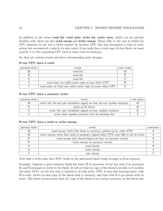
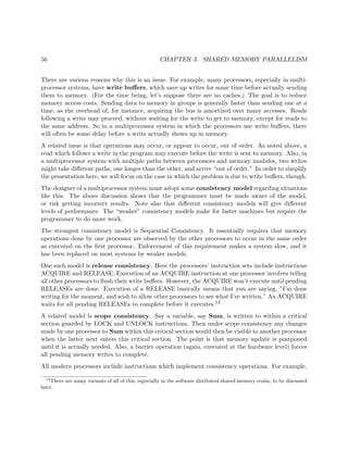
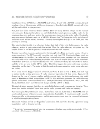
9 // Unix compilation: gcc -g -o primesthreads PrimesThreads.c -lpthread -lm
10
11 // usage: primesthreads n num_threads
12
13 #include <stdio.h>
14 #include <math.h>
15 #include <pthread.h> // required for threads usage
16
17 #define MAX_N 100000000
18 #define MAX_THREADS 25
19
20 // shared variables
21 int nthreads, // number of threads (not counting main())
22 n, // range to check for primeness
23 prime[MAX_N+1], // in the end, prime[i] = 1 if i prime, else 0
24 nextbase; // next sieve multiplier to be used
25 // lock for the shared variable nextbase
26 pthread_mutex_t nextbaselock = PTHREAD_MUTEX_INITIALIZER;
27 // ID structs for the threads
28 pthread_t id[MAX_THREADS];
3
There may be other processes running too. So the threads of our program must still take turns with other
processes running on the machine.](https://image.slidesharecdn.com/matloff-programmingonparallelmachines-2013-150626072019-lva1-app6892/85/Matloff-programming-on-parallel_machines-2013-27-320.jpg)
![8 CHAPTER 1. INTRODUCTION TO PARALLEL PROCESSING
29
30 // "crosses out" all odd multiples of k
31 void crossout(int k)
32 { int i;
33 for (i = 3; i*k <= n; i += 2) {
34 prime[i*k] = 0;
35 }
36 }
37
38 // each thread runs this routine
39 void *worker(int tn) // tn is the thread number (0,1,...)
40 { int lim,base,
41 work = 0; // amount of work done by this thread
42 // no need to check multipliers bigger than sqrt(n)
43 lim = sqrt(n);
44 do {
45 // get next sieve multiplier, avoiding duplication across threads
46 // lock the lock
47 pthread_mutex_lock(&nextbaselock);
48 base = nextbase;
49 nextbase += 2;
50 // unlock
51 pthread_mutex_unlock(&nextbaselock);
52 if (base <= lim) {
53 // don’t bother crossing out if base known composite
54 if (prime[base]) {
55 crossout(base);
56 work++; // log work done by this thread
57 }
58 }
59 else return work;
60 } while (1);
61 }
62
63 main(int argc, char **argv)
64 { int nprimes, // number of primes found
65 i,work;
66 n = atoi(argv[1]);
67 nthreads = atoi(argv[2]);
68 // mark all even numbers nonprime, and the rest "prime until
69 // shown otherwise"
70 for (i = 3; i <= n; i++) {
71 if (i%2 == 0) prime[i] = 0;
72 else prime[i] = 1;
73 }
74 nextbase = 3;
75 // get threads started
76 for (i = 0; i < nthreads; i++) {
77 // this call says create a thread, record its ID in the array
78 // id, and get the thread started executing the function worker(),
79 // passing the argument i to that function
80 pthread_create(&id[i],NULL,worker,i);
81 }
82
83 // wait for all done
84 for (i = 0; i < nthreads; i++) {
85 // this call says wait until thread number id[i] finishes
86 // execution, and to assign the return value of that thread to our](https://image.slidesharecdn.com/matloff-programmingonparallelmachines-2013-150626072019-lva1-app6892/85/Matloff-programming-on-parallel_machines-2013-28-320.jpg)
![1.3. PROGRAMMER WORLD VIEWS 9
87 // local variable work here
88 pthread_join(id[i],&work);
89 printf("%d values of base donen",work);
90 }
91
92 // report results
93 nprimes = 1;
94 for (i = 3; i <= n; i++)
95 if (prime[i]) {
96 nprimes++;
97 }
98 printf("the number of primes found was %dn",nprimes);
99
100 }
To make our discussion concrete, suppose we are running this program with two threads. Suppose
also the both threads are running simultaneously most of the time. This will occur if they aren’t
competing for turns with other threads, say if there are no other threads, or more generally if the
number of other threads is less than or equal to the number of processors minus two. (Actually,
the original thread is main(), but it lies dormant most of the time, as you’ll see.)
Note the global variables:
int nthreads, // number of threads (not counting main())
n, // range to check for primeness
prime[MAX_N+1], // in the end, prime[i] = 1 if i prime, else 0
nextbase; // next sieve multiplier to be used
pthread_mutex_t nextbaselock = PTHREAD_MUTEX_INITIALIZER;
pthread_t id[MAX_THREADS];
This will require some adjustment for those who’ve been taught that global variables are “evil.”
In most threaded programs, all communication between threads is done via global variables.4 So
even if you consider globals to be evil, they are a necessary evil in threads programming.
Personally I have always thought the stern admonitions against global variables are overblown any-
way; see http://heather.cs.ucdavis.edu/~matloff/globals.html. But as mentioned, those
admonitions are routinely ignored in threaded programming. For a nice discussion on this, see the
paper by a famous MIT computer scientist on an Intel Web page, at http://software.intel.
com/en-us/articles/global-variable-reconsidered/?wapkw=%28parallelism%29.
As mentioned earlier, the globals are shared by all processors.5 If one processor, for instance,
assigns the value 0 to prime[35] in the function crossout(), then that variable will have the value
4
Technically one could use locals in main() (or whatever function it is where the threads are created) for this
purpose, but this would be so unwieldy that it is seldom done.
5
Technically, we should say “shared by all threads” here, as a given thread does not always execute on the same
processor, but at any instant in time each executing thread is at some processor, so the statement is all right.](https://image.slidesharecdn.com/matloff-programmingonparallelmachines-2013-150626072019-lva1-app6892/85/Matloff-programming-on-parallel_machines-2013-29-320.jpg)
![1.3. PROGRAMMER WORLD VIEWS 11
• Both threads would do “crossing out” of multiples of 11, duplicating work and thus slowing
down execution speed.
• We will never “cross out” multiples of 13.
Thus the lock is crucial to the correct (and speedy) execution of the program.
Note that these problems could occur either on a uniprocessor or multiprocessor system. In the
uniprocessor case, thread A’s turn might end right after it reads nextbase, followed by a turn by
B which executes that same instruction. In the multiprocessor case, A and B could literally be
running simultaneously, but still with the action by B coming an instant after A.
This problem frequently arises in parallel database systems. For instance, consider an airline
reservation system. If a flight has only one seat left, we want to avoid giving it to two different
customers who might be talking to two agents at the same time. The lines of code in which the
seat is finally assigned (the commit phase, in database terminology) is then a critical section.
A critical section is always a potential bottleneck in a parallel program, because its code is serial
instead of parallel. In our program here, we may get better performance by having each thread
work on, say, five values of nextbase at a time. Our line
nextbase += 2;
would become
nextbase += 10;
That would mean that any given thread would need to go through the critical section only one-fifth
as often, thus greatly reducing overhead. On the other hand, near the end of the run, this may
result in some threads being idle while other threads still have a lot of work to do.
Note this code.
for (i = 0; i < nthreads; i++) {
pthread_join(id[i],&work);
printf("%d values of base donen",work);
}
This is a special case of of barrier.
A barrier is a point in the code that all threads must reach before continuing. In this case, a barrier
is needed in order to prevent premature execution of the later code](https://image.slidesharecdn.com/matloff-programmingonparallelmachines-2013-150626072019-lva1-app6892/85/Matloff-programming-on-parallel_machines-2013-31-320.jpg)
![12 CHAPTER 1. INTRODUCTION TO PARALLEL PROCESSING
for (i = 3; i <= n; i++)
if (prime[i]) {
nprimes++;
}
which would result in possibly wrong output if we start counting primes before some threads are
done.
Actually, we could have used Pthreads’ built-in barrier function. We need to declare a barrier
variable, e.g.
p t h r e a d b a r r i e r t barr ;
and then call it like this:
pthread barrier wait (&barr ) ;
The pthread join() function actually causes the given thread to exit, so that we then “join” the
thread that created it, i.e. main(). Thus some may argue that this is not really a true barrier.
Barriers are very common in shared-memory programming, and will be discussed in more detail in
Chapter 3.
1.3.2.3 Role of the OS
Let’s again ponder the role of the OS here. What happens when a thread tries to lock a lock:
• The lock call will ultimately cause a system call, causing the OS to run.
• The OS keeps track of the locked/unlocked status of each lock, so it will check that status.
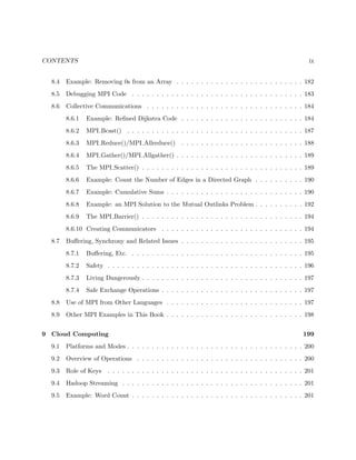
• Say the lock is unlocked (a 0). Then the OS sets it to locked (a 1), and the lock call returns.
The thread enters the critical section.
• When the thread is done, the unlock call unlocks the lock, similar to the locking actions.
• If the lock is locked at the time a thread makes a lock call, the call will block. The OS will
mark this thread as waiting for the lock. When whatever thread currently using the critical
section unlocks the lock, the OS will relock it and unblock the lock call of the waiting thread.
If several threads are waiting, of course only one will be unblock.
Note that main() is a thread too, the original thread that spawns the others. However, it is
dormant most of the time, due to its calls to pthread join().](https://image.slidesharecdn.com/matloff-programmingonparallelmachines-2013-150626072019-lva1-app6892/85/Matloff-programming-on-parallel_machines-2013-32-320.jpg)
![1.3. PROGRAMMER WORLD VIEWS 13
Finally, keep in mind that although the globals variables are shared, the locals are not. Recall that
local variables are stored on a stack. Each thread (just like each process in general) has its own
stack. When a thread begins a turn, the OS prepares for this by pointing the stack pointer register
to this thread’s stack.
1.3.2.4 Debugging Threads Programs
Most debugging tools include facilities for threads. Here’s an overview of how it works in GDB.
First, as you run a program under GDB, the creation of new threads will be announced, e.g.
(gdb) r 100 2
Starting program: /debug/primes 100 2
[New Thread 16384 (LWP 28653)]
[New Thread 32769 (LWP 28676)]
[New Thread 16386 (LWP 28677)]
[New Thread 32771 (LWP 28678)]
You can do backtrace (bt) etc. as usual. Here are some threads-related commands:
• info threads (gives information on all current threads)
• thread 3 (change to thread 3)
• break 88 thread 3 (stop execution when thread 3 reaches source line 88)
• break 88 thread 3 if x==y (stop execution when thread 3 reaches source line 88 and the
variables x and y are equal)
Of course, many GUI IDEs use GDB internally, and thus provide the above facilities with a GUI
wrapper. Examples are DDD, Eclipse and NetBeans.
1.3.2.5 Higher-Level Threads
The OpenMP library gives the programmer a higher-level view of threading. The threads are there,
but rather hidden by higher-level abstractions. We will study OpenMP in detail in Chapter 4, and
use it frequently in the succeeding chapters, but below is an introductory example.
1.3.2.6 Example: Sampling Bucket Sort
This code implements the sampling bucket sort of Section 12.5.](https://image.slidesharecdn.com/matloff-programmingonparallelmachines-2013-150626072019-lva1-app6892/85/Matloff-programming-on-parallel_machines-2013-33-320.jpg)
![14 CHAPTER 1. INTRODUCTION TO PARALLEL PROCESSING
1 // OpenMP introductory example : sampling bucket sort
2
3 // compile : gcc −fopenmp −o bsort bucketsort . c
4
5 // set the number of threads via the environment v a r i a b l e
6 // OMP NUM THREADS, e . g . in the C s h e l l
7
8 // setenv OMP NUM THREADS 8
9
10 #include <omp. h> // required
11 #include <s t d l i b . h>
12
13 // needed f o r c a l l to qsort ()
14 int cmpints ( int ∗u , int ∗v)
15 { i f (∗u < ∗v) return −1;
16 i f (∗u > ∗v) return 1;
17 return 0;
18 }
19
20 // adds xi to the part array , increments npart , the length of part
21 void grab ( int xi , int ∗part , int ∗ npart )
22 {
23 part [∗ npart ] = xi ;
24 ∗ npart += 1;
25 }
26
27 // f i n d s the min and max in y , length ny ,
28 // placing them in miny and maxy
29 void findminmax ( int ∗y , int ny , int ∗miny , int ∗maxy)
30 { int i , yi ;
31 ∗miny = ∗maxy = y [ 0 ] ;
32 f o r ( i = 1; i < ny ; i++) {
33 yi = y [ i ] ;
34 i f ( yi < ∗miny) ∗miny = yi ;
35 e l s e i f ( yi > ∗maxy) ∗maxy = yi ;
36 }
37 }
38
39 // sort the array x of length n
40 void bsort ( int ∗x , int n)
41 { // these are l o c a l to t h i s function , but shared among the threads
42 f l o a t ∗ bdries ; int ∗ counts ;
43 #pragma omp p a r a l l e l
44 // entering t h i s block a c t i v a t e s the threads , each executing i t
45 { // these are l o c a l to each thread :
46 int me = omp get thread num ( ) ;
47 int nth = omp get num threads ( ) ;
48 int i , xi , minx , maxx , s t a r t ;
49 int ∗mypart ;
50 f l o a t increm ;](https://image.slidesharecdn.com/matloff-programmingonparallelmachines-2013-150626072019-lva1-app6892/85/Matloff-programming-on-parallel_machines-2013-34-320.jpg)
![1.3. PROGRAMMER WORLD VIEWS 15
51 int SAMPLESIZE;
52 // now determine the bucket boundaries ; nth − 1 of them , by
53 // sampling the array to get an idea of i t s range
54 #pragma omp s i n g l e // only 1 thread does this , implied b a r r i e r at end
55 {
56 i f (n > 1000) SAMPLESIZE = 1000;
57 e l s e SAMPLESIZE = n / 2;
58 findminmax (x ,SAMPLESIZE,&minx,&maxx ) ;
59 bdries = malloc (( nth −1)∗ s i z e o f ( f l o a t ) ) ;
60 increm = (maxx − minx ) / ( f l o a t ) nth ;
61 f o r ( i = 0; i < nth −1; i++)
62 bdries [ i ] = minx + ( i +1) ∗ increm ;
63 // array to serve as the count of the numbers of elements of x
64 // in each bucket
65 counts = malloc ( nth∗ s i z e o f ( int ) ) ;
66 }
67 // now have t h i s thread grab i t s portion of the array ; thread 0
68 // takes everything below bdries [ 0 ] , thread 1 everything between
69 // bdries [ 0 ] and bdries [ 1 ] , etc . , with thread nth−1 taking
70 // everything over bdries [ nth −1]
71 mypart = malloc (n∗ s i z e o f ( int ) ) ; int nummypart = 0;
72 f o r ( i = 0; i < n ; i++) {
73 i f (me == 0) {
74 i f (x [ i ] <= bdries [ 0 ] ) grab (x [ i ] , mypart ,&nummypart ) ;
75 }
76 e l s e i f (me < nth −1) {
77 i f (x [ i ] > bdries [me−1] && x [ i ] <= bdries [me ] )
78 grab (x [ i ] , mypart ,&nummypart ) ;
79 } e l s e
80 i f (x [ i ] > bdries [me−1]) grab (x [ i ] , mypart ,&nummypart ) ;
81 }
82 // now record how many t h i s thread got
83 counts [me] = nummypart ;
84 // sort my part
85 qsort ( mypart , nummypart , s i z e o f ( int ) , cmpints ) ;
86 #pragma omp b a r r i e r // other threads need to know a l l of counts
87 // copy sorted chunk back to the o r i g i n a l array ; f i r s t find s t a r t point
88 s t a r t = 0;
89 f o r ( i = 0; i < me; i++) s t a r t += counts [ i ] ;
90 f o r ( i = 0; i < nummypart ; i++) {
91 x [ s t a r t+i ] = mypart [ i ] ;
92 }
93 }
94 // implied b a r r i e r here ; main thread won ’ t resume u n t i l a l l threads
95 // are done
96 }
97
98 int main ( int argc , char ∗∗ argv )
99 {
100 // t e s t case](https://image.slidesharecdn.com/matloff-programmingonparallelmachines-2013-150626072019-lva1-app6892/85/Matloff-programming-on-parallel_machines-2013-35-320.jpg)
![16 CHAPTER 1. INTRODUCTION TO PARALLEL PROCESSING
101 int n = a t o i ( argv [ 1 ] ) , ∗x = malloc (n∗ s i z e o f ( int ) ) ;
102 int i ;
103 f o r ( i = 0; i < n ; i++) x [ i ] = rand () % 50;
104 i f (n < 100)
105 f o r ( i = 0; i < n ; i++) p r i n t f (”%dn” ,x [ i ] ) ;
106 bsort (x , n ) ;
107 i f (n <= 100) {
108 p r i n t f (”x a f t e r s o r t i n g : n ” ) ;
109 f o r ( i = 0; i < n ; i++) p r i n t f (”%dn” ,x [ i ] ) ;
110 }
111 }
Details on OpenMP are presented in Chapter 4. Here is an overview of a few of the OpenMP
constructs available:
• #pragma omp for
In our example above, we wrote our own code to assign specific threads to do specific parts
of the work. An alternative is to write an ordinary for loop that iterates over all the work to
be done, and then ask OpenMP to assign specific iterations to specific threads. To do this,
insert the above pragma just before the loop.
• #pragma omp critical
The block that follows is implemented as a critical section. OpenMP sets up the locks etc.
for you, alleviating you of work and alleviating your code of clutter.
1.3.3 Message Passing
1.3.3.1 Programmer View
Again consider the matrix-vector multiply example of Section 1.3.1. In contrast to the shared-
memory case, in the message-passing paradigm all nodes would have separate copies of A, X and
Y. Our example in Section 1.3.2.1 would now change. in order for node 2 to send this new value of
Y[3] to node 15, it would have to execute some special function, which would be something like
send(15,12,"Y[3]");
and node 15 would have to execute some kind of receive() function.
To compute the matrix-vector product, then, would involve the following. One node, say node 0,
would distribute the rows of A to the various other nodes. Each node would receive a different set](https://image.slidesharecdn.com/matloff-programmingonparallelmachines-2013-150626072019-lva1-app6892/85/Matloff-programming-on-parallel_machines-2013-36-320.jpg)
![18 CHAPTER 1. INTRODUCTION TO PARALLEL PROCESSING
35 N, // find all primes from 2 to N
36 Me; // my node number
37 double T1,T2; // start and finish times
38
39 void Init(int Argc,char **Argv)
40 { int DebugWait;
41 N = atoi(Argv[1]);
42 // start debugging section
43 DebugWait = atoi(Argv[2]);
44 while (DebugWait) ; // deliberate infinite loop; see below
45 /* the above loop is here to synchronize all nodes for debugging;
46 if DebugWait is specified as 1 on the mpirun command line, all
47 nodes wait here until the debugging programmer starts GDB at
48 all nodes (via attaching to OS process number), then sets
49 some breakpoints, then GDB sets DebugWait to 0 to proceed; */
50 // end debugging section
51 MPI_Init(&Argc,&Argv); // mandatory to begin any MPI program
52 // puts the number of nodes in NNodes
53 MPI_Comm_size(MPI_COMM_WORLD,&NNodes);
54 // puts the node number of this node in Me
55 MPI_Comm_rank(MPI_COMM_WORLD,&Me);
56 // OK, get started; first record current time in T1
57 if (Me == NNodes-1) T1 = MPI_Wtime();
58 }
59
60 void Node0()
61 { int I,ToCheck,Dummy,Error;
62 for (I = 1; I <= N/2; I++) {
63 ToCheck = 2 * I + 1; // latest number to check for div3
64 if (ToCheck > N) break;
65 if (ToCheck % 3 > 0) // not divis by 3, so send it down the pipe
66 // send the string at ToCheck, consisting of 1 MPI integer, to
67 // node 1 among MPI_COMM_WORLD, with a message type PIPE_MSG
68 Error = MPI_Send(&ToCheck,1,MPI_INT,1,PIPE_MSG,MPI_COMM_WORLD);
69 // error not checked in this code
70 }
71 // sentinel
72 MPI_Send(&Dummy,1,MPI_INT,1,END_MSG,MPI_COMM_WORLD);
73 }
74
75 void NodeBetween()
76 { int ToCheck,Dummy,Divisor;
77 MPI_Status Status;
78 // first received item gives us our prime divisor
79 // receive into Divisor 1 MPI integer from node Me-1, of any message
80 // type, and put information about the message in Status
81 MPI_Recv(&Divisor,1,MPI_INT,Me-1,MPI_ANY_TAG,MPI_COMM_WORLD,&Status);
82 while (1) {
83 MPI_Recv(&ToCheck,1,MPI_INT,Me-1,MPI_ANY_TAG,MPI_COMM_WORLD,&Status);
84 // if the message type was END_MSG, end loop
85 if (Status.MPI_TAG == END_MSG) break;
86 if (ToCheck % Divisor > 0)
87 MPI_Send(&ToCheck,1,MPI_INT,Me+1,PIPE_MSG,MPI_COMM_WORLD);
88 }
89 MPI_Send(&Dummy,1,MPI_INT,Me+1,END_MSG,MPI_COMM_WORLD);
90 }
91
92 NodeEnd()](https://image.slidesharecdn.com/matloff-programmingonparallelmachines-2013-150626072019-lva1-app6892/85/Matloff-programming-on-parallel_machines-2013-38-320.jpg)
![20 CHAPTER 1. INTRODUCTION TO PARALLEL PROCESSING
1.3.4 Scatter/Gather
Technically, the scatter/gather programmer world view is a special case of message passing.
However, it has become so pervasive as to merit its own section here.
In this paradigm, one node, say node 0, serves as a manager, while the others serve as workers.
The parcels out work to the workers, who process their respective chunks of the data and return the
results to the manager. The latter receives the results and combines them into the final product.
The matrix-vector multiply example in Section 1.3.3.1 is an example of scatter/gather.
As noted, scatter/gather is very popular. Here are some examples of packages that use it:
• MPI includes scatter and gather functions (Section 7.4).
• Hadoop/MapReduce Computing (Chapter 9) is basically a scatter/gather operation.
• The snow package (Section 1.3.4.1) for the R language is also a scatter/gather operation.
1.3.4.1 R snow Package
Base R does not include parallel processing facilities, but includes the parallel library for this
purpose, and a number of other parallel libraries are available as well. The parallel package
arose from the merger (and slight modifcation) of two former user-contributed libraries, snow and
multicore. The former (and essentially the latter) uses the scatter/gather paradigm, and so will
be introduced in this section; see Section 1.3.4.1 for further details. for convenience, I’ll refer to
the portion of parallel that came from snow simply as snow.
Let’s use matrix-vector multiply as an example to learn from:
1 > l i b r a r y ( p a r a l l e l )
2 > c2 <− makePSOCKcluster ( rep (” l o c a l h o s t ” ,2))
3 > c2
4 socket c l u s t e r with 2 nodes on host l o c a l h o s t
5 > mmul
6 function ( cls , u , v) {
7 rowgrps <− s p l i t I n d i c e s ( nrow (u ) , length ( c l s ))
8 grpmul <− function ( grp ) u [ grp , ] %∗% v
9 mout <− clusterApply ( cls , rowgrps , grpmul )
10 Reduce ( c , mout)
11 }
12 > a <− matrix ( sample (1:50 ,16 , replace=T) , ncol =2)
13 > a
14 [ , 1 ] [ , 2 ]
15 [ 1 , ] 34 41
16 [ 2 , ] 10 28](https://image.slidesharecdn.com/matloff-programmingonparallelmachines-2013-150626072019-lva1-app6892/85/Matloff-programming-on-parallel_machines-2013-40-320.jpg)
![1.3. PROGRAMMER WORLD VIEWS 21
17 [ 3 , ] 44 23
18 [ 4 , ] 7 29
19 [ 5 , ] 6 24
20 [ 6 , ] 28 29
21 [ 7 , ] 21 1
22 [ 8 , ] 38 30
23 > b <− c (5 , −2)
24 > b
25 [ 1 ] 5 −2
26 > a %∗% b # s e r i a l multiply
27 [ , 1 ]
28 [ 1 , ] 88
29 [ 2 , ] −6
30 [ 3 , ] 174
31 [ 4 , ] −23
32 [ 5 , ] −18
33 [ 6 , ] 82
34 [ 7 , ] 103
35 [ 8 , ] 130
36 > clusterExport ( c2 , c (” a ” ,”b ”)) # send a , b to workers
37 > clusterEvalQ ( c2 , a ) # check that they have i t
38 [ [ 1 ] ]
39 [ , 1 ] [ , 2 ]
40 [ 1 , ] 34 41
41 [ 2 , ] 10 28
42 [ 3 , ] 44 23
43 [ 4 , ] 7 29
44 [ 5 , ] 6 24
45 [ 6 , ] 28 29
46 [ 7 , ] 21 1
47 [ 8 , ] 38 30
48
49 [ [ 2 ] ]
50 [ , 1 ] [ , 2 ]
51 [ 1 , ] 34 41
52 [ 2 , ] 10 28
53 [ 3 , ] 44 23
54 [ 4 , ] 7 29
55 [ 5 , ] 6 24
56 [ 6 , ] 28 29
57 [ 7 , ] 21 1
58 [ 8 , ] 38 30
59 > mmul( c2 , a , b) # t e s t our p a r a l l e l code
60 [ 1 ] 88 −6 174 −23 −18 82 103 130
What just happened?
First we set up a snow cluster. The term should not be confused with hardware systems we referred
to as “clusters” earlier. We are simply setting up a group of R processes that will communicate](https://image.slidesharecdn.com/matloff-programmingonparallelmachines-2013-150626072019-lva1-app6892/85/Matloff-programming-on-parallel_machines-2013-41-320.jpg)
![22 CHAPTER 1. INTRODUCTION TO PARALLEL PROCESSING
with each other via TCP/IP sockets.
In this case, my cluster consists of two R processes running on the machine from which I invoked
makePSOCKcluster(). (In TCP/IP terminology, localhost refers to the local machine.) If I
were to run the Unix ps command, with appropriate options, say ax, I’d see three R processes. I
saved the cluster in c2.
On the other hand, my snow cluster could indeed be set up on a real cluster, e.g.
c3 <− makePSOCKcluster ( c (” pc28 ” ,” pc29 ” ,” pc29 ”))
where pc28 etc. are machine names.
In preparing to test my parallel code, I needed to ship my matrices a and b to the workers:
> clusterExport ( c2 , c (” a ” ,”b ”)) # send a , b to workers
Note that this function assumes that a and b are global variables at the invoking node, i.e. the
manager, and it will place copies of them in the global workspace of the worker nodes.
Note that the copies are independent of the originals; if a worker changes, say, b[3], that change
won’t be made at the manager or at the other worker. This is a message-passing system, indeed.
So, how does the mmul code work? Here’s a handy copy:
1 mmul <− function ( cls , u , v) {
2 rowgrps <− s p l i t I n d i c e s ( nrow (u ) , length ( c l s ))
3 grpmul <− function ( grp ) u [ grp , ] %∗% v
4 mout <− clusterApply ( cls , rowgrps , grpmul )
5 Reduce ( c , mout)
6 }
As discussed in Section 1.3.1, our strategy will be to partition the rows of the matrix, and then
have different workers handle different groups of rows. Our call to splitIndices() sets this up for
us.
That function does what its name implies, e.g.
> s p l i t I n d i c e s (12 ,5)
[ [ 1 ] ]
[ 1 ] 1 2 3
[ [ 2 ] ]
[ 1 ] 4 5
[ [ 3 ] ]
[ 1 ] 6 7
[ [ 4 ] ]
[ 1 ] 8 9](https://image.slidesharecdn.com/matloff-programmingonparallelmachines-2013-150626072019-lva1-app6892/85/Matloff-programming-on-parallel_machines-2013-42-320.jpg)
![1.3. PROGRAMMER WORLD VIEWS 23
[ [ 5 ] ]
[ 1 ] 10 11 12
Here we asked the function to partition the numbers 1,...,12 into 5 groups, as equal-sized as possible,
which you can see is what it did. Note that the type of the return value is an R list.
So, after executing that function in our mmul() code, rowgrps will be an R list consisting of a
partitioning of the row numbers of u, exactly what we need.
The call to clusterApply() is then where the actual work is assigned to the workers. The code
mout <− clusterApply ( cls , rowgrps , grpmul )
instructs snow to have the first worker process the rows in rowgrps[[1]], the second worker to
work on rowgrps[[2]], and so on. The clusterApply() function expects its second argument to
be an R list, which is the case here.
Each worker will then multiply v by its row group, and return the product to the manager. However,
the product will again be a list, one component for each worker, so we need Reduce() to string
everything back together.
Note that R does allow functions defined within functions, which the locals and arguments of the
outer function becoming global to the inner function.
Note that a here could have been huge, in which case the export action could slow down our
program. If a were not needed at the workers other than for this one-time matrix multiply, we may
wish to change to code so that we send each worker only the rows of a that we need:
1 mmul1 <− function ( cls , u , v) {
2 rowgrps <− s p l i t I n d i c e s ( nrow (u ) , length ( c l s ))
3 uchunks <− Map( function ( grp ) u [ grp , ] , rowgrps )
4 mulchunk <− function ( uc ) uc %∗% v
5 mout <− clusterApply ( cls , uchunks , mulchunk )
6 Reduce ( c , mout)
7 }
Let’s test it:
1 > a <− matrix ( sample (1:50 ,16 , replace=T) , ncol =2)
2 > b <− c (5 , −2)
3 > clusterExport ( c2 ,” b”) # don ’ t send a
4 a
5 [ , 1 ] [ , 2 ]
6 [ 1 , ] 10 26
7 [ 2 , ] 1 34
8 [ 3 , ] 49 30
9 [ 4 , ] 39 41
10 [ 5 , ] 12 14](https://image.slidesharecdn.com/matloff-programmingonparallelmachines-2013-150626072019-lva1-app6892/85/Matloff-programming-on-parallel_machines-2013-43-320.jpg)
![24 CHAPTER 1. INTRODUCTION TO PARALLEL PROCESSING
11 [ 6 , ] 2 30
12 [ 7 , ] 33 23
13 [ 8 , ] 44 5
14 > a %∗% b
15 [ , 1 ]
16 [ 1 , ] −2
17 [ 2 , ] −63
18 [ 3 , ] 185
19 [ 4 , ] 113
20 [ 5 , ] 32
21 [ 6 , ] −50
22 [ 7 , ] 119
23 [ 8 , ] 210
24 > mmul1( c2 , a , b)
25 [ 1 ] −2 −63 185 113 32 −50 119 210
Note that we did not need to use clusterExport() to send the chunks of a to the workers, as the
call to clusterApply() does this, since it sends the arguments,](https://image.slidesharecdn.com/matloff-programmingonparallelmachines-2013-150626072019-lva1-app6892/85/Matloff-programming-on-parallel_machines-2013-44-320.jpg)
![2.4. STATIC (BUT POSSIBLY RANDOM) TASK ASSIGNMENT TYPICALLY BETTER THAN DYNAMIC31
In the Mandelbrot example, we could randomly assign rows of the picture, in the same way, and
avoid load imbalance.
So, actually, Method A, or let’s call it Method A’, will still typically work well.
2.4.3 Example: Mutual Web Outlinks
Here’s an example that we’ll use at various points in this book:
Mutual outlinks in a graph:
Consider a network graph of some kind, such as Web links. For any two vertices, say
any two Web sites, we might be interested in mutual outlinks, i.e. outbound links that
are common to two Web sites. Say we want to find the number of mutual outlinks,
averaged over all pairs of Web sites.
Let A be the adjacency matrix of the graph. Then the mean of interest would be
found as follows:
1 sum = 0
2 f o r i = 0 . . . n−2
3 f o r j = i + 1 . . . n−1
4 count = 0
5 f o r k = 0 . . . n−1 count += a [ i ] [ k ] ∗ a [ j ] [ k ]
6 mean = sum / (n∗(n−1)/2)
Say again n = 10000 and we have 10 threads. We should not simply assign work to the
threads by dividing up the i loop, with thread 0 taking the cases i = 0,...,999, thread
1 the cases 1000,...,1999 and so on. This would give us a real load balance problem.
Thread 8 would have much less work to do than thread 3, say.
We could randomize as discussed earlier, but there is a much better solution: Just pair
the rows of A. Thread 0 would handle rows 0,...,499 and 9500,...,9999, thread 1 would
handle rows 500,999 and 9000,...,9499 etc. This approach is taken in our OpenMP
implementation, Section 4.12.
In other words, Method A still works well.
In the mutual outlinks problem, we have a good idea beforehand as to how much time each task
needs, but this may not be true in general. An alternative would be to do random pre-assignment
of tasks to processors.
On the other hand, if we know beforehand that all of the tasks should take about the same time,
we should use static scheduling, as it might yield better cache and virtual memory performance.](https://image.slidesharecdn.com/matloff-programmingonparallelmachines-2013-150626072019-lva1-app6892/85/Matloff-programming-on-parallel_machines-2013-51-320.jpg)
![3.2. MEMORY MODULES 37
(a) High-order interleaving: Here consecutive words are in the same bank (except at bound-
aries). For example, suppose for simplicity that our memory consists of word-addresses 0
through 1023, and that there are four banks, M0 through M3. Then M0 would contain
word-addresses 0-255, M1 would have 256-511, M2 would have 512-767, and M3 would have
768-1023.
(b) Low-order interleaving: Here consecutive addresses are in consecutive banks (except when
we get to the right end). In the example above, if we used low-order interleaving, then word-
address 0 would be in M0, 1 would be in M1, 2 would be in M2, 3 would be in M3, 4 would
be back in M0, 5 in M1, and so on.
Say we have eight banks. Then under high-order interleaving, the first three bits of a word-address
would be taken to be the bank number, with the remaining bits being address within bank. Under
low-order interleaving, the three least significant bits would be used to determine bank number.
Low-order interleaving has often been used for vector processors. On such a machine, we might
have both a regular add instruction, ADD, and a vector version, VADD. The latter would add two
vectors together, so it would need to read two vectors from memory. If low-order interleaving is
used, the elements of these vectors are spread across the various banks, so fast access is possible.
A more modern use of low-order interleaving, but with the same motivation as with the vector
processors, is in GPUs (Chapter 5).
High-order interleaving might work well in matrix applications, for instance, where we can partition
the matrix into blocks, and have different processors work on different blocks. In image processing
applications, we can have different processors work on different parts of the image. Such partitioning
almost never works perfectly—e.g. computation for one part of an image may need information
from another part—but if we are careful we can get good results.
3.2.2 Bank Conflicts and Solutions
Consider an array x of 16 million elements, whose sum we wish to compute, say using 16 threads.
Suppose we have four memory banks, with low-order interleaving.
A naive implementation of the summing code might be
1 parallel for thr = 0 to 15
2 localsum = 0
3 for j = 0 to 999999
4 localsum += x[thr*1000000+j]
5 grandsum += localsumsum
In other words, thread 0 would sum the first million elements, thread 1 would sum the second
million, and so on. After summing its portion of the array, a thread would then add its sum to a](https://image.slidesharecdn.com/matloff-programmingonparallelmachines-2013-150626072019-lva1-app6892/85/Matloff-programming-on-parallel_machines-2013-57-320.jpg)
![38 CHAPTER 3. SHARED MEMORY PARALLELISM
grand total. (The threads could of course add to grandsum directly in each iteration of the loop,
but this would cause too much traffic to memory, thus causing slowdowns.)
Suppose for simplicity that the threads run in lockstep, so that they all attempt to access memory
at once. On a multicore/multiprocessor machine, this may not occur, but it in fact typically will
occur in a GPU setting.
A problem then arises. To make matters simple, suppose that x starts at an address that is a
multiple of 4, thus in bank 0. (The reader should think about how to adjust this to the other
three cases.) On the very first memory access, thread 0 accesses x[0] in bank 0, thread 1 accesses
x[1000000], also in bank 0, and so on—and these will all be in memory bank 0! Thus there will
be major conflicts, hence major slowdown.
A better approach might be to have any given thread work on every sixteenth element of x, instead
of on contiguous elements. Thread 0 would work on x[1000000], x[1000016], x[10000032,...;
thread 1 would handle x[1000001], x[1000017], x[10000033,...; and so on:
1 parallel for thr = 0 to 15
2 localsum = 0
3 for j = 0 to 999999
4 localsum += x[16*j+thr]
5 grandsum += localsumsum
Here, consecutive threads work on consecutive elements in x.1 That puts them in separate banks,
thus no conflicts, hence speedy performance.
In general, avoiding bank conflicts is an art, but there are a couple of approaches we can try.
• We can rewrite our algorithm, e.g. use the second version of the above code instead of the
first.
• We can add padding to the array. For instance in the first version of our code above, we
could lengthen the array from 16 million to 16000016, placing padding in words 1000000,
2000001 and so on. We’d tweak our array indices in our code accordingly, and eliminate bank
conflicts that way.
In the first approach above, the concept of stride often arises. It is defined to be the distance
betwwen array elements in consecutive accesses by a thread. In our original code to compute
grandsum, the stride was 1, since each array element accessed by a thread is 1 past the last access
by that thread. In our second version, the stride was 16.
Strides of greater than 1 often arise in code that deals with multidimensional arrays. Say for
example we have two-dimensional array with 16 columns. In C/C++, which uses row-major order,
1
Here thread 0 is considered “consecutive” to thread 15, in a wraparound manner.](https://image.slidesharecdn.com/matloff-programmingonparallelmachines-2013-150626072019-lva1-app6892/85/Matloff-programming-on-parallel_machines-2013-58-320.jpg)
![3.2. MEMORY MODULES 39
access of an entire column will have a stride of 16. Access down the main diagonal will have a
stride of 17.
Suppose we have b banks, again with low-order interleaving. You should experiment a bit to see
that an array access with a stride of s will access s different banks if and only if s and b are relatively
prime, i.e. the greatest common divisor of s and b is 1. This can be proven with group theory.
Another strategy, useful for collections of complex objects, is to set up structs of arrays rather
than arrays of structs. Say for instance we are working with data on workers, storing for each
worker his name, salary and number of years with the firm. We might naturally write code like
this:
1 s t r u c t {
2 char name [ 2 5 ] ;
3 f l o a t salary ;
4 f l o a t yrs ;
5 } x [ 1 0 0 ] ;
That gives a 100 structs for 100 workers. Again, this is very natural, but it may make for poor
memory access patterns. Salary values for the various workers will no longer be contiguous, for
instance, even though the structs are contiguous. This could cause excessive cache misses.
One solution would be to add padding to each struct, so that the salary values are a word apart
in memory. But another approach would be to replace the above arrays of structs by a struct of
arrays:
1 s t r u c t {
2 char ∗name [ ] 1 0 0 ;
3 f l o a t salary [ 1 0 0 ] ;
4 f l o a t yrs [ 1 0 0 ] ;
5 }
3.2.3 Example: Code to Implement Padding
As discussed above, array padding is used to try to get better parallel access to memory banks. The
code below is aimed to provide utilities to assist in this. Details are explained in the comments.
1
2 // routines to i n i t i a l i z e , read and write
3 // padded versions of a matrix of f l o a t s ;
4 // the matrix i s nominally mxn, but i t s
5 // rows w i l l be padded on the r i g h t ends ,
6 // so as to enable a s t r i d e of s down each
7 // column ; i t i s assumed that s >= n
8
9 // a l l o c a t e space f o r the padded matrix ,](https://image.slidesharecdn.com/matloff-programmingonparallelmachines-2013-150626072019-lva1-app6892/85/Matloff-programming-on-parallel_machines-2013-59-320.jpg)
![52 CHAPTER 3. SHARED MEMORY PARALLELISM
time it does the TAS, until P6 leaves the critical section, writes 0 to L, and causes another cache
miss at P5, etc.
At first the update approach seems obviously superior, and actually, if our shared, cacheable10
variables were only lock variables, this might be true.
But consider a shared, cacheable vector. Suppose the vector fits into one block, and that we write
to each vector element sequentially. Under an update policy, we would have to send a new message
on the bus/network for each component, while under an invalidate policy, only one message (for the
first component) would be needed. If during this time the other processors do not need to access
this vector, all those update messages, and the bus/network bandwidth they use, would be wasted.
Or suppose for example we have code like
Sum += X[I];
in the middle of a for loop. Under an update protocol, we would have to write the value of Sum
back many times, even though the other processors may only be interested in the final value when
the loop ends. (This would be true, for instance, if the code above were part of a critical section.)
Thus the invalidate protocol works well for some kinds of code, while update works better for
others. The CPU designers must try to anticipate which protocol will work well across a broad mix
of applications.11
Now, how is cache coherency handled in non-bus shared-memory systems, say crossbars? Here
the problem is more complex. Think back to the bus case for a minute: The very feature which
was the biggest negative feature of bus systems—the fact that there was only one path between
components made bandwidth very limited—is a very positive feature in terms of cache coherency,
because it makes broadcast very easy: Since everyone is attached to that single pathway, sending a
message to all of them costs no more than sending it to just one—we get the others for free. That’s
no longer the case for multipath systems. In such systems, extra copies of the message must be
created for each path, adding to overall traffic.
A solution is to send messages only to “interested parties.” In directory-based protocols, a list is
kept of all caches which currently have valid copies of all blocks. In one common implementation, for
example, while P2 is in the critical section above, it would be the owner of the block containing L.
(Whoever is the latest node to write to L would be considered its current owner.) It would maintain
a directory of all caches having valid copies of that block, say C5 and C6 in our story here. As
soon as P2 wrote to L, it would then send either invalidate or update packets (depending on which
type was being used) to C5 and C6 (and not to other caches which didn’t have valid copies).
10
Many modern processors, including Pentium and MIPS, allow the programmer to mark some blocks as being
noncacheable.
11
Some protocols change between the two modes dynamically.](https://image.slidesharecdn.com/matloff-programmingonparallelmachines-2013-150626072019-lva1-app6892/85/Matloff-programming-on-parallel_machines-2013-72-320.jpg)
![3.6. MEMORY-ACCESS CONSISTENCY POLICIES 55
has state I at A. B’s action does not cause loading of that block from memory to its cache, so the
block still has state I at B.
3.5.3 The Problem of “False Sharing”
Consider the C declaration
int W,Z;
Since W and Z are declared adjacently, most compilers will assign them contiguous memory ad-
dresses. Thus, unless one of them is at a memory block boundary, when they are cached they
will be stored in the same cache line. Suppose the program writes to Z, and our system uses an
invalidate protocol. Then W will be considered invalid at the other processors, even though its
values at those processors’ caches are correct. This is the false sharing problem, alluding to the
fact that the two variables are sharing a cache line even though they are not related.
This can have very adverse impacts on performance. If for instance our variable W is now written
to, then Z will suffer unfairly, as its copy in the cache will be considered invalid even though it is
perfectly valid. This can lead to a “ping-pong” effect, in which alternate writing to two variables
leads to a cyclic pattern of coherency transactions.
One possible solution is to add padding, e.g. declaring W and Z like this:
int Q,U[1000],Z;
to separate Q and Z so that they won’t be in the same cache block. Of course, we must take block
size into account, and check whether the compiler really has placed the two variables are in widely
separated locations. To do this, we could for instance run the code
printf("%x %xn,&Q,&Z);
3.6 Memory-Access Consistency Policies
Though the word consistency in the title of this section may seem to simply be a synonym for
coherency from the last section, and though there actually is some relation, the issues here are
quite different. In this case, it is a timing issue: After one processor changes the value of a shared
variable, when will that value be visible to the other processors?](https://image.slidesharecdn.com/matloff-programmingonparallelmachines-2013-150626072019-lva1-app6892/85/Matloff-programming-on-parallel_machines-2013-75-320.jpg)
![60 CHAPTER 3. SHARED MEMORY PARALLELISM
SDSM itself is divided into two main approaches, the page-based and object-based varieties.
The page-based approach is generally considered clearer and easier to program in, and provides the
programmer the “look and feel” of shared-memory programming better than does the object-based
type.16 We will discuss only the page-based approach here. The most popular SDSM system today
is the page-based Treadmarks (Rice University). Another excellent page-based system is JIAJIA
(Academy of Sciences, China).
To illustrate how page-based SDSMs work, consider the line of JIAJIA code
Prime = (int *) jia_alloc(N*sizeof(int));
The function jia alloc() is part of the JIAJIA library, libjia.a, which is linked to one’s application
program during compilation.
At first this looks a little like a call to the standard malloc() function, setting up an array Prime
of size N. In fact, it does indeed allocate some memory. Note that each node in our JIAJIA group
is executing this statement, so each node allocates some memory at that node. Behind the scenes,
not visible to the programmer, each node will then have its own copy of Prime.
However, JIAJIA sets things up so that when one node later accesses this memory, for instance in
the statement
Prime[I] = 1;
this action will eventually trigger a network transaction (not visible to the programmer) to the
other JIAJIA nodes.17 This transaction will then update the copies of Prime at the other nodes.18
How is all of this accomplished? It turns out that it relies on a clever usage of the nodes’ virtual
memory (VM) systems. To understand this, you need a basic knowledge of how VM systems work.
If you lack this, or need review, read Section A.2.2 in the appendix of this book before continuing.
Here is how VM is exploited to develop SDSMs on Unix systems. The SDSM will call a system
function such as mprotect(). This allows the SDSM to deliberately mark a page as nonresident
(even if the page is resident). Basically, anytime the SDSM knows that a node’s local copy of a
variable is invalid, it will mark the page containing that variable as nonresident. Then, the next
time the program at this node tries to access that variable, a page fault will occur.
As mentioned in the review above, normally a page fault causes a jump to the OS. However,
technically any page fault in Unix is handled as a signal, specifically SIGSEGV. Recall that Unix
allows the programmer to write his/her own signal handler for any signal type. In this case, that
16
The term object-based is not related to the term object-oriented programming.
17
There are a number of important issues involved with this word eventually, as we will see later.
18
The update may not occur immediately. More on this later.](https://image.slidesharecdn.com/matloff-programmingonparallelmachines-2013-150626072019-lva1-app6892/85/Matloff-programming-on-parallel_machines-2013-80-320.jpg)
![62 CHAPTER 3. SHARED MEMORY PARALLELISM
3.11.0.2 Case Study: JIAJIA
Programmer Interface
We will not go into detail on JIAJIA programming here. There is a short tutorial on JIAJIA at
http://heather.cs.ucdavis.edu/~matloff/jiajia.html, but here is an overview:
• One writes in C/C++ (or FORTRAN), making calls to the JIAJIA library, which is linked
in upon compilation.
• The library calls include standard shared-memory operations for lock, unlock, barrier, pro-
cessor number, etc., plus some calls aimed at improving performance.
Following is a JIAJIA example program, performing Odd/Even Transposition Sort. This is a
variant on Bubble Sort, sometimes useful in parallel processing contexts.20 The algorithm consists
of n phases, in which each processor alternates between trading with its left and right neighbors.
1 // JIAJIA example program: Odd-Even Tranposition Sort
2
3 // array is of size n, and we use n processors; this would be more
4 // efficient in a "chunked" versions, of course (and more suited for a
5 // message-passing context anyway)
6
7 #include <stdio.h>
8 #include <stdlib.h>
9 #include <jia.h> // required include; also must link via -ljia
10
11 // pointer to shared variable
12 float *x; // array to be sorted
13
14 int n, // range to check for primeness
15 debug; // 1 for debugging, 0 else
16
17
18 // does sort of m-element array y
19 void oddeven(float *y, int m)
20 { int i,left=jiapid-1,right=jiapid+1;
21 float newval;
22 for (i=0; i < m; i++) {
23 if ((i+jiapid)%2 == 0) {
24 if (right < m)
25 if (y[jiapid] > y[right]) newval = y[right];
26 }
27 else {
28 if (left >= 0)
29 if (y[jiapid] < y[left]) newval = y[left];
30 }
31 jia_barrier();
20
Though, as mentioned in the comments, it is aimed more at message-passing contexts.](https://image.slidesharecdn.com/matloff-programmingonparallelmachines-2013-150626072019-lva1-app6892/85/Matloff-programming-on-parallel_machines-2013-82-320.jpg)
![3.11. ILLUSION OF SHARED-MEMORY THROUGH SOFTWARE 63
32 if ((i+jiapid)%2 == 0 && right < m || (i+jiapid)%2 == 1 && left >= 0)
33 y[jiapid] = newval;
34 jia_barrier();
35 }
36 }
37
38 main(int argc, char **argv)
39 { int i,mywait=0;
40 jia_init(argc,argv); // required init call
41 // get command-line arguments (shifted for nodes > 0)
42 if (jiapid == 0) {
43 n = atoi(argv[1]);
44 debug = atoi(argv[2]);
45 }
46 else {
47 n = atoi(argv[2]);
48 debug = atoi(argv[3]);
49 }
50 jia_barrier();
51 // create a shared array x of length n
52 x = (float *) jia_alloc(n*sizeof(float));
53 // barrier recommended after allocation
54 jia_barrier();
55 // node 0 gets simple test array from command-line
56 if (jiapid == 0) {
57 for (i = 0; i < n; i++)
58 x[i] = atoi(argv[i+3]);
59 }
60 jia_barrier();
61 if (debug && jiapid == 0)
62 while (mywait == 0) { ; }
63 jia_barrier();
64 oddeven(x,n);
65 if (jiapid == 0) {
66 printf("nfinal arrayn");
67 for (i = 0; i < n; i++)
68 printf("%fn",x[i]);
69 }
70 jia_exit();
71 }
System Workings
JIAJIA’s main characteristics as an SDSM are:
• page-based
• scope consistency
• home-based
• multiple writers](https://image.slidesharecdn.com/matloff-programmingonparallelmachines-2013-150626072019-lva1-app6892/85/Matloff-programming-on-parallel_machines-2013-83-320.jpg)
![3.12. BARRIER IMPLEMENTATION 67
if we are unlucky, some other processor, say processor 3, will then race ahead, perform the second
iteration of the loop in an extremely short period of time, and then reach the barrier and increment
the Count variable before processor 12 resets it to 0. This would result in disaster, since processor
3’s increment would be canceled, leaving us one short when we try to finish the barrier the second
time.
Another disaster scenario which might occur is that one processor might reset B.Count to 0 before
another processor had a chance to notice that B.Count had reached B.NNodes.
3.12.3 A Correct Version
One way to avoid this would be to have two Count variables, and have the processors alternate
using one then the other. In the scenario described above, processor 3 would increment the other
Count variable, and thus would not conflict with processor 12’s resetting. Here is a safe barrier
function based on this idea:
1 struct BarrStruct {
2 int NNodes, // number of threads participating in the barrier
3 Count[2], // number of threads that have hit the barrier so far
4 pthread_mutex_t Lock = PTHREAD_MUTEX_INITIALIZER;
5 } ;
6
7 Barrier(struct BarrStruct *PB)
8 { int Par,OldCount;
9 Par = PB->EvenOdd;
10 pthread_mutex_lock(&PB->Lock);
11 OldCount = PB->Count[Par]++;
12 if (OldCount == PB->NNodes-1) {
13 PB->Count[Par] = 0;
14 PB->EvenOdd = 1 - Par;
15 pthread_mutex_unlock(&PB->Lock);
16 }
17 else {
18 pthread_mutex_unlock(&PB->Lock);
19 while (PB->Count[Par] > 0) ;
20 }
21 }
3.12.4 Refinements
3.12.4.1 Use of Wait Operations
The code
else while (PB->Count[Par] > 0) ;](https://image.slidesharecdn.com/matloff-programmingonparallelmachines-2013-150626072019-lva1-app6892/85/Matloff-programming-on-parallel_machines-2013-87-320.jpg)
![68 CHAPTER 3. SHARED MEMORY PARALLELISM
is harming performance, since it has the processor spining around doing no useful work. In the
Pthreads context, we can use a condition variable:
1 struct BarrStruct {
2 int NNodes, // number of threads participating in the barrier
3 Count[2], // number of threads that have hit the barrier so far
4 pthread_mutex_t Lock = PTHREAD_MUTEX_INITIALIZER;
5 pthread_cond_t CV = PTHREAD_COND_INITIALIZER;
6 } ;
7
8 Barrier(struct BarrStruct *PB)
9 { int Par,I;
10 Par = PB->EvenOdd;
11 pthread_mutex_lock(&PB->Lock);
12 PB->Count[Par]++;
13 if (PB->Count < PB->NNodes)
14 pthread_cond_wait(&PB->CV,&PB->Lock);
15 else {
16 PB->Count[Par] = 0;
17 PB->EvenOdd = 1 - Par;
18 for (I = 0; I < PB->NNodes-1; I++)
19 pthread_cond_signal(&PB->CV);
20 }
21 pthread_mutex_unlock(&PB->Lock);
22 }
Here, if a thread finds that not everyone has reached the barrier yet, it still waits for the rest, but
does so passively, via the wait for the condition variable CV. This way the thread is not wasting
valuable time on that processor, which can run other useful work.
Note that the call to pthread cond wait() requires use of the lock. Your code must lock the
lock before making the call. The call itself immediately unlocks that lock after it registers the
wait with the threads manager. But the call blocks until awakened when another thread calls
pthread cond signal() or pthread cond broadcast().
It is required that your code lock the lock before calling pthread cond signal(), and that it
unlock the lock after the call.
By using pthread cond wait() and placing the unlock operation later in the code, as seen above,
we actually could get by with just a single Count variable, as before.
Even better, the for loop could be replaced by a single call
pthread_cond_broadcast(&PB->CV);
This still wakes up the waiting threads one by one, but in a much more efficient way, and it makes
for clearer code.](https://image.slidesharecdn.com/matloff-programmingonparallelmachines-2013-150626072019-lva1-app6892/85/Matloff-programming-on-parallel_machines-2013-88-320.jpg)
![3.12. BARRIER IMPLEMENTATION 69
3.12.4.2 Parallelizing the Barrier Operation
3.12.4.2.1 Tree Barriers It is clear from the code above that barriers can be costly to per-
formance, since they rely so heavily on critical sections, i.e. serial parts of a program. Thus in
many settings it is worthwhile to parallelize not only the general computation, but also the barrier
operations themselves.
Consider for instance a barrier in which 16 threads are participating. We could speed things up
by breaking this barrier down into two sub-barriers, with eight threads each. We would then set
up three barrier operations: one of the first group of eight threads, another for the other group
of eight threads, and a third consisting of a “competition” between the two groups. The variable
NNodes above would have the value 8 for the first two barriers, and would be equal to 2 for the
third barrier.
Here thread 0 could be the representative for the first group, with thread 4 representing the second
group. After both groups’s barriers were hit by all of their members, threads 0 and 4 would
participated in the third barrier.
Note that then the notification phase would the be done in reverse: When the third barrier was
complete, threads 0 and 4 would notify the members of their groups.
This would parallelize things somewhat, as critical-section operations could be executing simulta-
neously for the first two barriers. There would still be quite a bit of serial action, though, so we
may wish to do further splitting, by partitioning each group of four threads into two subroups of
two threads each.
In general, for n threads (with n, say, equal to a power of 2) we would have a tree structure, with
log2n levels in the tree. The ith level (starting with the root as level 0) with consist of 2i parallel
barriers, each one representing n/2i threads.
3.12.4.2.2 Butterfly Barriers Another method basically consists of each node “shaking hands”
with every other node. In the shared-memory case, handshaking could be done by having a global
array ReachedBarrier. When thread 3 and thread 7 shake hands, for instance, would reach the
barrier, thread 3 would set ReachedBarrier[3] to 1, and would then wait for ReachedBarrier[7]
to become 1. The wait, as before, could either be a while loop or a call to pthread cond wait().
Thread 7 would do the opposite.
If we have n nodes, again with n being a power of 2, then the barrier process would consist of log2n
phases, which we’ll call phase 0, phase 1, etc. Then the process works as follows.
For any node i, let i(k) be the number obtained by inverting bit k in the binary representation of
i, with bit 0 being the least significant bit. Then in the kth phase, node i would shake hands with
node i(k).](https://image.slidesharecdn.com/matloff-programmingonparallelmachines-2013-150626072019-lva1-app6892/85/Matloff-programming-on-parallel_machines-2013-89-320.jpg)

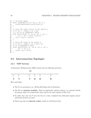
![72 CHAPTER 4. INTRODUCTION TO OPENMP
4 // bidirectional graph; finds the shortest path from vertex 0 to all
5 // others
6
7 // usage: dijkstra nv print
8
9 // where nv is the size of the graph, and print is 1 if graph and min
10 // distances are to be printed out, 0 otherwise
11
12 #include <omp.h>
13
14 // global variables, shared by all threads by default
15
16 int nv, // number of vertices
17 *notdone, // vertices not checked yet
18 nth, // number of threads
19 chunk, // number of vertices handled by each thread
20 md, // current min over all threads
21 mv, // vertex which achieves that min
22 largeint = -1; // max possible unsigned int
23
24 unsigned *ohd, // 1-hop distances between vertices; "ohd[i][j]" is
25 // ohd[i*nv+j]
26 *mind; // min distances found so far
27
28 void init(int ac, char **av)
29 { int i,j,tmp;
30 nv = atoi(av[1]);
31 ohd = malloc(nv*nv*sizeof(int));
32 mind = malloc(nv*sizeof(int));
33 notdone = malloc(nv*sizeof(int));
34 // random graph
35 for (i = 0; i < nv; i++)
36 for (j = i; j < nv; j++) {
37 if (j == i) ohd[i*nv+i] = 0;
38 else {
39 ohd[nv*i+j] = rand() % 20;
40 ohd[nv*j+i] = ohd[nv*i+j];
41 }
42 }
43 for (i = 1; i < nv; i++) {
44 notdone[i] = 1;
45 mind[i] = ohd[i];
46 }
47 }
48
49 // finds closest to 0 among notdone, among s through e
50 void findmymin(int s, int e, unsigned *d, int *v)
51 { int i;
52 *d = largeint;
53 for (i = s; i <= e; i++)
54 if (notdone[i] && mind[i] < *d) {
55 *d = mind[i];
56 *v = i;
57 }
58 }
59
60 // for each i in [s,e], ask whether a shorter path to i exists, through
61 // mv](https://image.slidesharecdn.com/matloff-programmingonparallelmachines-2013-150626072019-lva1-app6892/85/Matloff-programming-on-parallel_machines-2013-92-320.jpg)
![4.2. EXAMPLE: DIJKSTRA SHORTEST-PATH ALGORITHM 73
62 void updatemind(int s, int e)
63 { int i;
64 for (i = s; i <= e; i++)
65 if (mind[mv] + ohd[mv*nv+i] < mind[i])
66 mind[i] = mind[mv] + ohd[mv*nv+i];
67 }
68
69 void dowork()
70 {
71 #pragma omp parallel
72 { int startv,endv, // start, end vertices for my thread
73 step, // whole procedure goes nv steps
74 mymv, // vertex which attains the min value in my chunk
75 me = omp_get_thread_num();
76 unsigned mymd; // min value found by this thread
77 #pragma omp single
78 { nth = omp_get_num_threads(); // must call inside parallel block
79 if (nv % nth != 0) {
80 printf("nv must be divisible by nthn");
81 exit(1);
82 }
83 chunk = nv/nth;
84 printf("there are %d threadsn",nth);
85 }
86 startv = me * chunk;
87 endv = startv + chunk - 1;
88 for (step = 0; step < nv; step++) {
89 // find closest vertex to 0 among notdone; each thread finds
90 // closest in its group, then we find overall closest
91 #pragma omp single
92 { md = largeint; mv = 0; }
93 findmymin(startv,endv,&mymd,&mymv);
94 // update overall min if mine is smaller
95 #pragma omp critical
96 { if (mymd < md)
97 { md = mymd; mv = mymv; }
98 }
99 #pragma omp barrier
100 // mark new vertex as done
101 #pragma omp single
102 { notdone[mv] = 0; }
103 // now update my section of mind
104 updatemind(startv,endv);
105 #pragma omp barrier
106 }
107 }
108 }
109
110 int main(int argc, char **argv)
111 { int i,j,print;
112 double startime,endtime;
113 init(argc,argv);
114 startime = omp_get_wtime();
115 // parallel
116 dowork();
117 // back to single thread
118 endtime = omp_get_wtime();
119 printf("elapsed time: %fn",endtime-startime);](https://image.slidesharecdn.com/matloff-programmingonparallelmachines-2013-150626072019-lva1-app6892/85/Matloff-programming-on-parallel_machines-2013-93-320.jpg)
![74 CHAPTER 4. INTRODUCTION TO OPENMP
120 print = atoi(argv[2]);
121 if (print) {
122 printf("graph weights:n");
123 for (i = 0; i < nv; i++) {
124 for (j = 0; j < nv; j++)
125 printf("%u ",ohd[nv*i+j]);
126 printf("n");
127 }
128 printf("minimum distances:n");
129 for (i = 1; i < nv; i++)
130 printf("%un",mind[i]);
131 }
132 }
The constructs will be presented in the following sections, but first the algorithm will be explained.
4.2.1 The Algorithm
The code implements the Dijkstra algorithm for finding the shortest paths from vertex 0 to the
other vertices in an N-vertex undirected graph. Pseudocode for the algorithm is shown below, with
the array G assumed to contain the one-hop distances between vertices.
1 Done = {0} # vertices checked so far
2 NewDone = None # currently checked vertex
3 NonDone = {1,2,...,N-1} # vertices not checked yet
4 for J = 0 to N-1 Dist[J] = G(0,J) # initialize shortest-path lengths
5
6 for Step = 1 to N-1
7 find J such that Dist[J] is min among all J in NonDone
8 transfer J from NonDone to Done
9 NewDone = J
10 for K = 1 to N-1
11 if K is in NonDone
12 # check if there is a shorter path from 0 to K through NewDone
13 # than our best so far
14 Dist[K] = min(Dist[K],Dist[NewDone]+G[NewDone,K])
At each iteration, the algorithm finds the closest vertex J to 0 among all those not yet processed,
and then updates the list of minimum distances to each vertex from 0 by considering paths that go
through J. Two obvious potential candidate part of the algorithm for parallelization are the “find
J” and “for K” lines, and the above OpenMP code takes this approach.
4.2.2 The OpenMP parallel Pragma
As can be seen in the comments in the lines](https://image.slidesharecdn.com/matloff-programmingonparallelmachines-2013-150626072019-lva1-app6892/85/Matloff-programming-on-parallel_machines-2013-94-320.jpg)
![78 CHAPTER 4. INTRODUCTION TO OPENMP
4 // in a bidirectional graph; finds the shortest path from vertex 0 to
5 // all others
6
7 // usage: dijkstra nv print
8
9 // where nv is the size of the graph, and print is 1 if graph and min
10 // distances are to be printed out, 0 otherwise
11
12 #include <omp.h>
13
14 // global variables, shared by all threads by default
15
16 int nv, // number of vertices
17 *notdone, // vertices not checked yet
18 nth, // number of threads
19 chunk, // number of vertices handled by each thread
20 md, // current min over all threads
21 mv, // vertex which achieves that min
22 largeint = -1; // max possible unsigned int
23
24 unsigned *ohd, // 1-hop distances between vertices; "ohd[i][j]" is
25 // ohd[i*nv+j]
26 *mind; // min distances found so far
27
28 void init(int ac, char **av)
29 { int i,j,tmp;
30 nv = atoi(av[1]);
31 ohd = malloc(nv*nv*sizeof(int));
32 mind = malloc(nv*sizeof(int));
33 notdone = malloc(nv*sizeof(int));
34 // random graph
35 for (i = 0; i < nv; i++)
36 for (j = i; j < nv; j++) {
37 if (j == i) ohd[i*nv+i] = 0;
38 else {
39 ohd[nv*i+j] = rand() % 20;
40 ohd[nv*j+i] = ohd[nv*i+j];
41 }
42 }
43 for (i = 1; i < nv; i++) {
44 notdone[i] = 1;
45 mind[i] = ohd[i];
46 }
47 }
48
49 void dowork()
50 {
51 #pragma omp parallel
52 { int step, // whole procedure goes nv steps
53 mymv, // vertex which attains that value
54 me = omp_get_thread_num(),
55 i;
56 unsigned mymd; // min value found by this thread
57 #pragma omp single
58 { nth = omp_get_num_threads();
59 printf("there are %d threadsn",nth); }
60 for (step = 0; step < nv; step++) {
61 // find closest vertex to 0 among notdone; each thread finds](https://image.slidesharecdn.com/matloff-programmingonparallelmachines-2013-150626072019-lva1-app6892/85/Matloff-programming-on-parallel_machines-2013-98-320.jpg)
![4.3. THE OPENMP FOR PRAGMA 79
62 // closest in its group, then we find overall closest
63 #pragma omp single
64 { md = largeint; mv = 0; }
65 mymd = largeint;
66 #pragma omp for nowait
67 for (i = 1; i < nv; i++) {
68 if (notdone[i] && mind[i] < mymd) {
69 mymd = ohd[i];
70 mymv = i;
71 }
72 }
73 // update overall min if mine is smaller
74 #pragma omp critical
75 { if (mymd < md)
76 { md = mymd; mv = mymv; }
77 }
78 // mark new vertex as done
79 #pragma omp single
80 { notdone[mv] = 0; }
81 // now update ohd
82 #pragma omp for
83 for (i = 1; i < nv; i++)
84 if (mind[mv] + ohd[mv*nv+i] < mind[i])
85 mind[i] = mind[mv] + ohd[mv*nv+i];
86 }
87 }
88 }
89
90 int main(int argc, char **argv)
91 { int i,j,print;
92 init(argc,argv);
93 // parallel
94 dowork();
95 // back to single thread
96 print = atoi(argv[2]);
97 if (print) {
98 printf("graph weights:n");
99 for (i = 0; i < nv; i++) {
100 for (j = 0; j < nv; j++)
101 printf("%u ",ohd[nv*i+j]);
102 printf("n");
103 }
104 printf("minimum distances:n");
105 for (i = 1; i < nv; i++)
106 printf("%un",mind[i]);
107 }
108 }
109
The work which used to be done in the function findmymin() is now done here:
#pragma omp for
for (i = 1; i < nv; i++) {
if (notdone[i] && mind[i] < mymd) {
mymd = ohd[i];
mymv = i;](https://image.slidesharecdn.com/matloff-programmingonparallelmachines-2013-150626072019-lva1-app6892/85/Matloff-programming-on-parallel_machines-2013-99-320.jpg)
![4.3. THE OPENMP FOR PRAGMA 81
For the Dijkstra algorithm, for instance, we could get the same operation with less code by asking
OpenMP to do the chunking for us, say with a chunk size of 8:
...
#pragma omp for schedule(static)
for (i = 1; i < nv; i++) {
if (notdone[i] && mind[i] < mymd) {
mymd = ohd[i];
mymv = i;
}
}
...
#pragma omp for schedule(static)
for (i = 1; i < nv; i++)
if (mind[mv] + ohd[mv*nv+i] < mind[i])
mind[i] = mind[mv] + ohd[mv*nv+i];
...
Note again that this would have the same effect as our original code, which each thread handling
one chunk of contiguous iterations within a loop. So it’s just a programming convenience for us in
this case. (If the number of threads doesn’t evenly divide the number of iterations, OpenMP will
fix that up for us too.)
The more general form is
#pragma omp for schedule(static,chunk)
Here static is still a keyword but chunk is an actual argument. However, setting the chunk size
in the schedule() clause is a compile-time operation. If you wish to have the chunk size set at run
time, call omp set schedule() in conjunction with the runtime clause. Example:
1 int main ( int argc , char ∗∗ argv )
2 {
3 . . .
4 n = a t oi ( argv [ 1 ] ) ;
5 int chunk = a to i ( argv [ 2 ] ) ;
6 omp set schedule ( omp sched static , chunk ) ;
7 #pragma omp p a r a l l e l
8 {
9 . . .
10 #pragma omp f o r schedule ( runtime )
11 f o r ( i = 1; i < n ; i++) {
12 . . .
13 }
14 . . .
15 }
16 }](https://image.slidesharecdn.com/matloff-programmingonparallelmachines-2013-150626072019-lva1-app6892/85/Matloff-programming-on-parallel_machines-2013-101-320.jpg)
![82 CHAPTER 4. INTRODUCTION TO OPENMP
Or set the OMP SCHEDULE environment variable.
The syntax is the same for dynamic and guided.
As discussed in Section 2.4, on the one hand, large chunks are good, due to there being less
overhead—every time a thread finishes a chunk, it must go through the critical section, which
serializes our parallel program and thus slows things down. On the other hand, if chunk sizes are
large, then toward the end of the work, some threads may be working on their last chunks while
others have finished and are now idle, thus foregoing potential speed enhancement. So it would be
nice to have large chunks at the beginning of the run, to reduce the overhead, but smaller chunks
at the end. This can be done using the guided clause.
For the Dijkstra algorithm, for instance, we could have this:
...
#pragma omp for schedule(guided)
for (i = 1; i < nv; i++) {
if (notdone[i] && mind[i] < mymd) {
mymd = ohd[i];
mymv = i;
}
}
...
#pragma omp for schedule(guided)
for (i = 1; i < nv; i++)
if (mind[mv] + ohd[mv*nv+i] < mind[i])
mind[i] = mind[mv] + ohd[mv*nv+i];
...
There are other variations of this available in OpenMP. However, in Section 2.4, I showed that
these would seldom be necessary or desirable; having each thread handle a single chunk would be
best.
See Section 2.4 for a timing example.
1 setenv OMP SCHEDULE ” s t a t i c ,20”
4.3.4 Example: In-Place Matrix Transpose
This method works in-place, a virtue if we are short on memory. Its cache performance is probably
poor, though. It may be better to look at horizontal slabs above the diagonal, say, and trade them
with vertical ones below the diagonal.
1 #include <omp. h>
2
3 // t r a n s l a t e from 2−D to 1−D i n d i c e s
4 int onedim ( int n , int i , int j ) { return n ∗ i + j ; }](https://image.slidesharecdn.com/matloff-programmingonparallelmachines-2013-150626072019-lva1-app6892/85/Matloff-programming-on-parallel_machines-2013-102-320.jpg)
![4.3. THE OPENMP FOR PRAGMA 83
5
6 void transp ( int ∗m, int n)
7 {
8 #pragma omp p a r a l l e l
9 { int i , j , tmp ;
10 // walk through a l l the above−diagonal elements , swapping them
11 // with t h e i r below−diagonal counterparts
12 #pragma omp f o r
13 f o r ( i = 0; i < n ; i++) {
14 f o r ( j = i +1; j < n ; j++) {
15 tmp = m[ onedim (n , i , j ) ] ;
16 m[ onedim (n , i , j ) ] = m[ onedim (n , j , i ) ] ;
17 m[ onedim (n , j , i ) ] = tmp ;
18 }
19 }
20 }
21 }
4.3.5 The OpenMP reduction Clause
The name of this OpenMP clause alludes to the term reduction in functional programming.
Many parallel programming languages include such operations, to enable the programmer to more
conveniently (and often more efficiently) have threads/processors cooperate in computing sums,
products, etc. OpenMP does this via the reduction clause.
For example, consider
1 int z;
2 ...
3 #pragma omp for reduction(+:z)
4 for (i = 0; i < n; i++) z += x[i];
The pragma says that the threads will share the work as in our previous discussion of the for
pragma. In addition, though, there will be independent copies of z maintained for each thread,
each initialized to 0 before the loop begins. When the loop is entirely done, the values of z from
the various threads will be summed, of course in an atomic manner.
Note that the + operator not only indicates that the values of z are to be summed, but also that
their initial values are to be 0. If the operator were *, say, then the product of the values would
be computed, and their initial values would be 1.
One can specify several reduction variables to the right of the colon, separated by commas.
Our use of the reduction clause here makes our programming much easier. Indeed, if we had old
serial code that we wanted to parallelize, we would have to make no change to it! OpenMP is taking](https://image.slidesharecdn.com/matloff-programmingonparallelmachines-2013-150626072019-lva1-app6892/85/Matloff-programming-on-parallel_machines-2013-103-320.jpg)
![84 CHAPTER 4. INTRODUCTION TO OPENMP
care of both the work splitting across values of i, and the atomic operations. Moreover—note this
carefully—it is efficient, because by maintaining separate copies of z until the loop is done, we are
reducing the number of serializing atomic actions, and are avoiding time-costly cache coherency
transactions and the like.
Without this construct, we would have to do
int z,myz=0;
...
#pragma omp for private(myz)
for (i = 0; i < n; i++) myz += x[i];
#pragma omp critical
{ z += myz; }
Here are the eligible operators and the corresponding initial values:
In C/C++, you can use reduction with +, -, *, &, |, && and || (and the exclusive-or operator).
operator initial value
+ 0
- 0
* 1
& bit string of 1s
| bit string of 0s
^ 0
&& 1
|| 0
The lack of other operations typically found in other parallel programming languages, such as min
and max, is due to the lack of these operators in C/C++. The FORTRAN version of OpenMP
does have min and max.3
Note that the reduction variables must be shared by the threads, and apparently the only acceptable
way to do so in this case is to declare them as global variables.
A reduction variable must be scalar, in C/C++. It can be an array in FORTRAN.
4.4 Example: Mandelbrot Set
Here’s the code for the timings in Section 2.4.5:
3
Note, though, that plain min and max would not help in our Dijkstra example above, as we not only need to find
the minimum value, but also need the vertex which attains that value.](https://image.slidesharecdn.com/matloff-programmingonparallelmachines-2013-150626072019-lva1-app6892/85/Matloff-programming-on-parallel_machines-2013-104-320.jpg)
![4.4. EXAMPLE: MANDELBROT SET 85
1 // compile with −D, e . g .
2 //
3 // gcc −fopenmp −o manddyn Gove . c −DDYNAMIC
4 //
5 // to get the version that uses dynamic scheduling
6
7 #include <omp. h>
8 #include <complex . h>
9
10 #include <time . h>
11 f l o a t t i m e d i f f ( s t r u c t timespec t1 , s t r u c t timespec t2 )
12 { i f ( t1 . tv nsec > t2 . tv nsec ) {
13 t2 . t v s e c −= 1;
14 t2 . tv nsec += 1000000000;
15 }
16 return t2 . tv sec −t1 . t v s e c + 0.000000001 ∗ ( t2 . tv nsec −t1 . tv nsec ) ;
17 }
18
19 #i f d e f RC
20 // f i n d s chunk among 0 , . . . , n−1 to assign to thread number me among nth
21 // threads
22 void findmyrange ( int n , int nth , int me, int ∗myrange )
23 { int chunksize = n / nth ;
24 myrange [ 0 ] = me ∗ chunksize ;
25 i f (me < nth −1) myrange [ 1 ] = (me+1) ∗ chunksize − 1;
26 e l s e myrange [ 1 ] = n − 1;
27 }
28
29 #include <s t d l i b . h>
30 #include <s t d i o . h>
31 // from http ://www. c i s . temple . edu/˜ ingargio / c i s 7 1 /code/randompermute . c
32 // I t returns a random permutation of 0 . . n−1
33 int ∗ rpermute ( int n) {
34 int ∗a = ( int ∗)( int ∗) malloc (n∗ s i z e o f ( int ) ) ;
35 // int ∗a = malloc (n∗ s i z e o f ( int ) ) ;
36 int k ;
37 f o r (k = 0; k < n ; k++)
38 a [ k ] = k ;
39 f o r (k = n−1; k > 0; k−−) {
40 int j = rand () % (k+1);
41 int temp = a [ j ] ;
42 a [ j ] = a [ k ] ;
43 a [ k ] = temp ;
44 }
45 return a ;
46 }
47 #endif
48
49 #define MAXITERS 1000
50](https://image.slidesharecdn.com/matloff-programmingonparallelmachines-2013-150626072019-lva1-app6892/85/Matloff-programming-on-parallel_machines-2013-105-320.jpg)
![86 CHAPTER 4. INTRODUCTION TO OPENMP
51 // g l o b a l s
52 int count = 0;
53 int nptsside ;
54 f l o a t side2 ;
55 f l o a t side4 ;
56
57 int i n s e t ( double complex c ) {
58 int i t e r s ;
59 f l o a t rl , im ;
60 double complex z = c ;
61 f o r ( i t e r s = 0; i t e r s < MAXITERS; i t e r s ++) {
62 z = z∗z + c ;
63 r l = c r e a l ( z ) ;
64 im = cimag ( z ) ;
65 i f ( r l ∗ r l + im∗im > 4) return 0;
66 }
67 return 1;
68 }
69
70 int ∗scram ;
71
72 void dowork ()
73 {
74 #i f d e f RC
75 #pragma omp p a r a l l e l reduction (+: count )
76 #e l s e
77 #pragma omp p a r a l l e l
78 #endif
79 {
80 int x , y ; f l o a t xv , yv ;
81 double complex z ;
82 #i f d e f STATIC
83 #pragma omp f o r reduction (+: count ) schedule ( s t a t i c )
84 #e l i f defined DYNAMIC
85 #pragma omp f o r reduction (+: count ) schedule ( dynamic )
86 #e l i f defined GUIDED
87 #pragma omp f o r reduction (+: count ) schedule ( guided )
88 #endif
89 #i f d e f RC
90 int myrange [ 2 ] ;
91 int me = omp get thread num ( ) ;
92 int nth = omp get num threads ( ) ;
93 int i ;
94 findmyrange ( nptsside , nth ,me, myrange ) ;
95 f o r ( i = myrange [ 0 ] ; i <= myrange [ 1 ] ; i++) {
96 x = scram [ i ] ;
97 #e l s e
98 f o r (x=0; x<nptsside ; x++) {
99 #endif
100 f o r ( y=0; y<nptsside ; y++) {](https://image.slidesharecdn.com/matloff-programmingonparallelmachines-2013-150626072019-lva1-app6892/85/Matloff-programming-on-parallel_machines-2013-106-320.jpg)
![4.5. THE TASK DIRECTIVE 87
101 xv = (x − side2 ) / side4 ;
102 yv = (y − side2 ) / side4 ;
103 z = xv + yv∗ I ;
104 i f ( i n s e t ( z )) {
105 count++;
106 }
107 }
108 }
109 }
110 }
111
112 int main ( int argc , char ∗∗ argv )
113 {
114 nptsside = at o i ( argv [ 1 ] ) ;
115 side2 = nptsside / 2 . 0 ;
116 side4 = nptsside / 4 . 0 ;
117
118 s t r u c t timespec bgn , nd ;
119 clock gettime (CLOCK REALTIME, &bgn ) ;
120
121 #i f d e f RC
122 scram = rpermute ( nptsside ) ;
123 #endif
124
125 dowork ( ) ;
126
127 // implied b a r r i e r
128 p r i n t f (”%dn” , count ) ;
129 clock gettime (CLOCK REALTIME, &nd ) ;
130 p r i n t f (”% f n” , t i m e d i f f (bgn , nd ) ) ;
131 }
The code is similar to that of a number of books and Web sites, such as the Gove book cited in
Section 2.2. Here RC is the random chunk method discussed in Section 2.4.
4.5 The Task Directive
This is new to OpenMP 3.0. The basic idea is to set up a task queue: When a thread encounters
a task directive, it arranges for some thread to execute the associated block—at some time. The
first thread can continue. Note that the task might not execute right away; it may have to wait
for some thread to become free after finishing another task. Also, there may be more tasks than
threads, also causing some threads to wait.
Note that we could arrange for all this ourselves, without task. We’d set up our own work queue,
as a shared variable, and write our code so that whenever a thread finished a unit of work, it would](https://image.slidesharecdn.com/matloff-programmingonparallelmachines-2013-150626072019-lva1-app6892/85/Matloff-programming-on-parallel_machines-2013-107-320.jpg)
![88 CHAPTER 4. INTRODUCTION TO OPENMP
delete the head of the queue. Whenever a thread generated a unit of work, it would add it to the
que. Of course, the deletion and addition would have to be done atomically. All this would amount
to a lot of coding on our part, so task really simplifies the programming.
4.5.1 Example: Quicksort
1 // OpenMP example program: quicksort; not necessarily efficient
2
3 void swap(int *yi, int *yj)
4 { int tmp = *yi;
5 *yi = *yj;
6 *yj = tmp;
7 }
8
9 int *separate(int *x, int low, int high)
10 { int i,pivot,last;
11 pivot = x[low]; // would be better to take, e.g., median of 1st 3 elts
12 swap(x+low,x+high);
13 last = low;
14 for (i = low; i < high; i++) {
15 if (x[i] <= pivot) {
16 swap(x+last,x+i);
17 last += 1;
18 }
19 }
20 swap(x+last,x+high);
21 return last;
22 }
23
24 // quicksort of the array z, elements zstart through zend; set the
25 // latter to 0 and m-1 in first call, where m is the length of z;
26 // firstcall is 1 or 0, according to whether this is the first of the
27 // recursive calls
28 void qs(int *z, int zstart, int zend, int firstcall)
29 {
30 #pragma omp parallel
31 { int part;
32 if (firstcall == 1) {
33 #pragma omp single nowait
34 qs(z,0,zend,0);
35 } else {
36 if (zstart < zend) {
37 part = separate(z,zstart,zend);
38 #pragma omp task
39 qs(z,zstart,part-1,0);
40 #pragma omp task
41 qs(z,part+1,zend,0);
42 }
43
44 }
45 }
46 }
47
48 // test code](https://image.slidesharecdn.com/matloff-programmingonparallelmachines-2013-150626072019-lva1-app6892/85/Matloff-programming-on-parallel_machines-2013-108-320.jpg)
![4.6. OTHER OPENMP SYNCHRONIZATION ISSUES 89
49 main(int argc, char**argv)
50 { int i,n,*w;
51 n = atoi(argv[1]);
52 w = malloc(n*sizeof(int));
53 for (i = 0; i < n; i++) w[i] = rand();
54 qs(w,0,n-1,1);
55 if (n < 25)
56 for (i = 0; i < n; i++) printf("%dn",w[i]);
57 }
The code
if (firstcall == 1) {
#pragma omp single nowait
qs(z,0,zend,0);
gets things going. We want only one thread to execute the root of the recursion tree, hence the
need for the single clause. After that, the code
part = separate(z,zstart,zend);
#pragma omp task
qs(z,zstart,part-1,0);
sets up a call to a subtree, with the task directive stating, “OMP system, please make sure that
this subtree is handled by some thread.”
There are various refinements, such as the barrier-like taskwait clause.
4.6 Other OpenMP Synchronization Issues
Earlier we saw the critical and barrier constructs. There is more to discuss, which we do here.
4.6.1 The OpenMP atomic Clause
The critical construct not only serializes your program, but also it adds a lot of overhead. If your
critical section involves just a one-statement update to a shared variable, e.g.
x += y;
etc., then the OpenMP compiler can take advantage of an atomic hardware instruction, e.g. the
LOCK prefix on Intel, to set up an extremely efficient critical section, e.g.](https://image.slidesharecdn.com/matloff-programmingonparallelmachines-2013-150626072019-lva1-app6892/85/Matloff-programming-on-parallel_machines-2013-109-320.jpg)
![94 CHAPTER 4. INTRODUCTION TO OPENMP
4.10.2 Some Fine Tuning
How could we make our Dijkstra code faster? One idea would be to eliminate the critical section.
Recall that in each iteration, the threads compute their local minimum distance values md and
mv, and then update the global values md and mv. Since the update must be atomic, this causes
some serialization of the program. Instead, we could have the threads store their values mymd
and mymv in a global array mymins, with each thread using a separate pair of locations within
that array, and then at the end of the iteration we could have just one task scan through mymins
and update md and mv.
Here is the resulting code:
1 // Dijkstra.c
2
3 // OpenMP example program: Dijkstra shortest-path finder in a
4 // bidirectional graph; finds the shortest path from vertex 0 to all
5 // others
6
7 // **** in this version, instead of having a critical section in which
8 // each thread updates md and mv, the threads record their mymd and mymv
9 // values in a global array mymins, which one thread then later uses to
10 // update md and mv
11
12 // usage: dijkstra nv print
13
14 // where nv is the size of the graph, and print is 1 if graph and min
15 // distances are to be printed out, 0 otherwise
16
17 #include <omp.h>
18
19 // global variables, shared by all threads by default
20
21 int nv, // number of vertices
22 *notdone, // vertices not checked yet
23 nth, // number of threads
24 chunk, // number of vertices handled by each thread
25 md, // current min over all threads
26 mv, // vertex which achieves that min
27 largeint = -1; // max possible unsigned int
28
29 int *mymins; // (mymd,mymv) for each thread; see dowork()
30
31 unsigned *ohd, // 1-hop distances between vertices; "ohd[i][j]" is
32 // ohd[i*nv+j]
33 *mind; // min distances found so far
34
35 void init(int ac, char **av)
36 { int i,j,tmp;
37 nv = atoi(av[1]);
38 ohd = malloc(nv*nv*sizeof(int));
39 mind = malloc(nv*sizeof(int));
40 notdone = malloc(nv*sizeof(int));
41 // random graph](https://image.slidesharecdn.com/matloff-programmingonparallelmachines-2013-150626072019-lva1-app6892/85/Matloff-programming-on-parallel_machines-2013-114-320.jpg)
![4.10. PERFORMANCE 95
42 for (i = 0; i < nv; i++)
43 for (j = i; j < nv; j++) {
44 if (j == i) ohd[i*nv+i] = 0;
45 else {
46 ohd[nv*i+j] = rand() % 20;
47 ohd[nv*j+i] = ohd[nv*i+j];
48 }
49 }
50 for (i = 1; i < nv; i++) {
51 notdone[i] = 1;
52 mind[i] = ohd[i];
53 }
54 }
55
56 // finds closest to 0 among notdone, among s through e
57 void findmymin(int s, int e, unsigned *d, int *v)
58 { int i;
59 *d = largeint;
60 for (i = s; i <= e; i++)
61 if (notdone[i] && mind[i] < *d) {
62 *d = ohd[i];
63 *v = i;
64 }
65 }
66
67 // for each i in [s,e], ask whether a shorter path to i exists, through
68 // mv
69 void updatemind(int s, int e)
70 { int i;
71 for (i = s; i <= e; i++)
72 if (mind[mv] + ohd[mv*nv+i] < mind[i])
73 mind[i] = mind[mv] + ohd[mv*nv+i];
74 }
75
76 void dowork()
77 {
78 #pragma omp parallel
79 { int startv,endv, // start, end vertices for my thread
80 step, // whole procedure goes nv steps
81 me,
82 mymv; // vertex which attains the min value in my chunk
83 unsigned mymd; // min value found by this thread
84 int i;
85 me = omp_get_thread_num();
86 #pragma omp single
87 { nth = omp_get_num_threads();
88 if (nv % nth != 0) {
89 printf("nv must be divisible by nthn");
90 exit(1);
91 }
92 chunk = nv/nth;
93 mymins = malloc(2*nth*sizeof(int));
94 }
95 startv = me * chunk;
96 endv = startv + chunk - 1;
97 for (step = 0; step < nv; step++) {
98 // find closest vertex to 0 among notdone; each thread finds
99 // closest in its group, then we find overall closest](https://image.slidesharecdn.com/matloff-programmingonparallelmachines-2013-150626072019-lva1-app6892/85/Matloff-programming-on-parallel_machines-2013-115-320.jpg)
![96 CHAPTER 4. INTRODUCTION TO OPENMP
100 findmymin(startv,endv,&mymd,&mymv);
101 mymins[2*me] = mymd;
102 mymins[2*me+1] = mymv;
103 #pragma omp barrier
104 // mark new vertex as done
105 #pragma omp single
106 { md = largeint; mv = 0;
107 for (i = 1; i < nth; i++)
108 if (mymins[2*i] < md) {
109 md = mymins[2*i];
110 mv = mymins[2*i+1];
111 }
112 notdone[mv] = 0;
113 }
114 // now update my section of mind
115 updatemind(startv,endv);
116 #pragma omp barrier
117 }
118 }
119 }
120
121 int main(int argc, char **argv)
122 { int i,j,print;
123 double startime,endtime;
124 init(argc,argv);
125 startime = omp_get_wtime();
126 // parallel
127 dowork();
128 // back to single thread
129 endtime = omp_get_wtime();
130 printf("elapsed time: %fn",endtime-startime);
131 print = atoi(argv[2]);
132 if (print) {
133 printf("graph weights:n");
134 for (i = 0; i < nv; i++) {
135 for (j = 0; j < nv; j++)
136 printf("%u ",ohd[nv*i+j]);
137 printf("n");
138 }
139 printf("minimum distances:n");
140 for (i = 1; i < nv; i++)
141 printf("%un",mind[i]);
142 }
143 }
Let’s take a look at the latter part of the code for one iteration;
1 findmymin(startv,endv,&mymd,&mymv);
2 mymins[2*me] = mymd;
3 mymins[2*me+1] = mymv;
4 #pragma omp barrier
5 // mark new vertex as done
6 #pragma omp single
7 { notdone[mv] = 0;
8 for (i = 1; i < nth; i++)
9 if (mymins[2*i] < md) {](https://image.slidesharecdn.com/matloff-programmingonparallelmachines-2013-150626072019-lva1-app6892/85/Matloff-programming-on-parallel_machines-2013-116-320.jpg)
![4.10. PERFORMANCE 97
10 md = mymins[2*i];
11 mv = mymins[2*i+1];
12 }
13 }
14 // now update my section of mind
15 updatemind(startv,endv);
16 #pragma omp barrier
The call to findmymin() is as before; this thread finds the closest vertex to 0 among this thread’s
range of vertices. But instead of comparing the result to md and possibly updating it and mv, the
thread simply stores its mymd and mymv in the global array mymins. After all threads have
done this and then waited at the barrier, we have just one thread update md and mv.
Let’s see how well this tack worked:
nv nth time
25000 1 2.546335
25000 2 1.449387
25000 4 1.411387
This brought us about a 15% speedup in the two-thread case, though less for four threads.
What else could we do? Here are a few ideas:
• False sharing could be a problem here. To address it, we could make mymins much longer,
changing the places at which the threads write their data, leaving most of the array as padding.
• We could try the modification of our program in Section 4.3.1, in which we use the OpenMP
for pragma, as well as the refinements stated there, such as schedule.
• We could try combining all of the ideas here.
4.10.3 OpenMP Internals
We may be able to write faster code if we know a bit about how OpenMP works inside.
You can get some idea of this from your compiler. For example, if you use the -t option with the
Omni compiler, or -k with Ompi, you can inspect the result of the preprocessing of the OpenMP
pragmas.
Here for instance is the code produced by Omni from the call to findmymin() in our Dijkstra
program:
# 93 "Dijkstra.c"
findmymin(startv,endv,&(mymd),&(mymv));{](https://image.slidesharecdn.com/matloff-programmingonparallelmachines-2013-150626072019-lva1-app6892/85/Matloff-programming-on-parallel_machines-2013-117-320.jpg)
![100 CHAPTER 4. INTRODUCTION TO OPENMP
58
59 int main ( int argc , char ∗∗ argv )
60 { p r i n t f (”% f n” , root ( t e s t f , −4.1 ,4.1 ,1000)); }
4.12 Example: Mutual Outlinks
Consider the example of Section 2.4.3. We have a network graph of some kind, such as Web
links. For any two vertices, say any two Web sites, we might be interested in mutual outlinks, i.e.
outbound links that are common to two Web sites.
The OpenMP code below finds the mean number of mutual outlinks, among all pairs of sites in a
set of Web sites. Note that it uses the method for load balancing presented in Section 2.4.3.
1 #include <omp.h>
2 #include <stdio.h>
3
4 // OpenMP example: finds mean number of mutual outlinks, among all
5 // pairs of Web sites in our set
6
7 int n, // number of sites (will assume n is even)
8 nth, // number of threads (will assume n/2 divisible by nth)
9 *m, // link matrix
10 tot = 0; // grand total of matches
11
12 // processes row pairs (i,i+1), (i,i+2), ...
13 int procpairs(int i)
14 { int j,k,sum=0;
15 for (j = i+1; j < n; j++) {
16 for (k = 0; k < n; k++)
17 sum += m[n*i+k] * m[n*j+k];
18 }
19 return sum;
20 }
21
22 float dowork()
23 {
24 #pragma omp parallel
25 { int pn1,pn2,i,mysum=0;
26 int me = omp_get_thread_num();
27 nth = omp_get_num_threads();
28 // in checking all (i,j) pairs, partition the work according to i;
29 // to get good load balance, this thread me will handle all i that equal
30 // me mod nth
31 for (i = me; i < n; i += nth) {
32 mysum += procpairs(i);
33 }
34 #pragma omp atomic
35 tot += mysum;
36 #pragma omp barrier
37 }
38 int divisor = n * (n-1) / 2;](https://image.slidesharecdn.com/matloff-programmingonparallelmachines-2013-150626072019-lva1-app6892/85/Matloff-programming-on-parallel_machines-2013-120-320.jpg)
![4.13. EXAMPLE: TRANSFORMING AN ADJACENCY MATRIX 101
39 return ((float) tot)/divisor;
40 }
41
42 int main(int argc, char **argv)
43 { int n2 = n/2,i,j;
44 n = atoi(argv[1]); // number of matrix rows/cols
45 int msize = n * n * sizeof(int);
46 m = (int *) malloc(msize);
47 // as a test, fill matrix with random 1s and 0s
48 for (i = 0; i < n; i++) {
49 m[n*i+i] = 0;
50 for (j = 0; j < n; j++) {
51 if (j != i) m[i*n+j] = rand() % 2;
52 }
53 }
54 if (n < 10) {
55 for (i = 0; i < n; i++) {
56 for (j = 0; j < n; j++) printf("%d ",m[n*i+j]);
57 printf("n");
58 }
59 }
60 tot = 0;
61 float meanml = dowork();
62 printf("mean = %fn",meanml);
63 }
4.13 Example: Transforming an Adjacency Matrix
Say we have a graph with adjacency matrix
0 1 0 0
1 0 0 1
0 1 0 1
1 1 1 0
(4.1)
with row and column numbering starting at 0, not 1. We’d like to transform this to a two-column
matrix that displays the links, in this case
0 1
1 0
1 3
2 1
2 3
3 0
3 1
3 2
(4.2)](https://image.slidesharecdn.com/matloff-programmingonparallelmachines-2013-150626072019-lva1-app6892/85/Matloff-programming-on-parallel_machines-2013-121-320.jpg)
![102 CHAPTER 4. INTRODUCTION TO OPENMP
For instance, there is a 1 on the far right, second row of the above matrix, meaning that in the
graph there is an edge from vertex 1 to vertex 3. This results in the row (1,3) in the transformed
matrix seen above.
Suppose further that we require this listing to be in lexicographical order, sorted on source vertex
and then on destination vertex. Here is code to do this computation in OpenMP:
1 // takes a graph adjacency matrix f o r a directed graph , and converts i t
2 // to a 2−column matrix of p a i r s ( i , j ) , meaning an edge from vertex i to
3 // vertex j ; the output matrix must be in l e x i c o g r a p h i c a l order
4
5 // not claimed e f f i c i e n t , e i t h e r in speed or in memory usage
6
7 #include <omp. h>
8
9 // needs −l r t l i n k f l a g f o r C++
10 #include <time . h>
11 f l o a t t i m e d i f f ( s t r u c t timespec t1 , s t r u c t timespec t2 )
12 { i f ( t1 . tv nsec > t2 . tv nsec ) {
13 t2 . t v s e c −= 1;
14 t2 . tv nsec += 1000000000;
15 }
16 return t2 . tv sec −t1 . t v s e c + 0.000000001 ∗ ( t2 . tv nsec −t1 . tv nsec ) ;
17 }
18
19 // transgraph () does t h i s work
20 // arguments :
21 // adjm : the adjacency matrix (NOT assumed symmetric ) , 1 f o r edge , 0
22 // otherwise ; note : matrix i s overwritten by the function
23 // n : number of rows and columns of adjm
24 // nout : output , number of rows in returned matrix
25 // return value : pointer to the converted matrix
26 int ∗ transgraph ( int ∗adjm , int n , int ∗nout )
27 {
28 int ∗outm , // to become the output matrix
29 ∗num1s , // i−th element w i l l be the number of 1 s in row i of adjm
30 ∗cumul1s ; // cumulative sums in num1s
31 #pragma omp p a r a l l e l
32 { int i , j ,m;
33 int me = omp get thread num ( ) ,
34 nth = omp get num threads ( ) ;
35 int myrows [ 2 ] ;
36 int tot1s ;
37 int outrow , num1si ;
38 #pragma omp s i n g l e
39 {
40 num1s = malloc (n∗ s i z e o f ( int ) ) ;
41 cumul1s = malloc (( n+1)∗ s i z e o f ( int ) ) ;
42 }
43 // determine the rows in adjm to be handled by t h i s thread](https://image.slidesharecdn.com/matloff-programmingonparallelmachines-2013-150626072019-lva1-app6892/85/Matloff-programming-on-parallel_machines-2013-122-320.jpg)
![4.13. EXAMPLE: TRANSFORMING AN ADJACENCY MATRIX 103
44 findmyrange (n , nth ,me, myrows ) ;
45 // s t a r t the action
46 f o r ( i = myrows [ 0 ] ; i <= myrows [ 1 ] ; i++) {
47 tot1s = 0;
48 f o r ( j = 0; j < n ; j++)
49 i f ( adjm [ n∗ i+j ] == 1) {
50 adjm [ n∗ i +( tot1s ++)] = j ;
51 }
52 num1s [ i ] = tot1s ;
53 }
54 #pragma omp b a r r i e r
55 #pragma omp s i n g l e
56 {
57 cumul1s [ 0 ] = 0;
58 // now c a l c u l a t e where the output of each row in adjm
59 // should s t a r t in outm
60 f o r (m = 1; m <= n ; m++) {
61 cumul1s [m] = cumul1s [m−1] + num1s [m−1];
62 }
63 ∗nout = cumul1s [ n ] ;
64 outm = malloc (2∗(∗ nout ) ∗ s i z e o f ( int ) ) ;
65 }
66 // now f i l l in t h i s thread ’ s portion
67 f o r ( i = myrows [ 0 ] ; i <= myrows [ 1 ] ; i++) {
68 outrow = cumul1s [ i ] ;
69 num1si = num1s [ i ] ;
70 f o r ( j = 0; j < num1si ; j++) {
71 outm [ 2 ∗ ( outrow+j ) ] = i ;
72 outm [ 2 ∗ ( outrow+j )+1] = adjm [ n∗ i+j ] ;
73 }
74 }
75 #pragma omp b a r r i e r
76 }
77 return outm ;
78 }
79
80 int main ( int argc , char ∗∗ argv )
81 { int i , j ;
82 int ∗adjm ;
83 int n = at o i ( argv [ 1 ] ) ;
84 int nout ;
85 int ∗outm ;
86 adjm = malloc (n∗n∗ s i z e o f ( int ) ) ;
87 f o r ( i = 0; i < n ; i++)
88 f o r ( j = 0; j < n ; j++)
89 i f ( i == j ) adjm [ n∗ i+j ] = 0;
90 e l s e adjm [ n∗ i+j ] = rand () % 2;
91
92 s t r u c t timespec bgn , nd ;
93 clock gettime (CLOCK REALTIME, &bgn ) ;](https://image.slidesharecdn.com/matloff-programmingonparallelmachines-2013-150626072019-lva1-app6892/85/Matloff-programming-on-parallel_machines-2013-123-320.jpg)
![104 CHAPTER 4. INTRODUCTION TO OPENMP
94
95 outm = transgraph (adjm , n,&nout ) ;
96 p r i n t f (”number of output rows : %dn” , nout ) ;
97
98 clock gettime (CLOCK REALTIME, &nd ) ;
99 p r i n t f (”% f n” , t i m e d i f f (bgn , nd ) ) ;
100
101 i f (n <= 10)
102 f o r ( i = 0; i < nout ; i++)
103 p r i n t f (”%d %dn” ,outm [2∗ i ] , outm [2∗ i +1]);
104 }
105
106 // f i n d s chunk among 0 , . . . , n−1 to assign to thread number me among nth
107 // threads
108 void findmyrange ( int n , int nth , int me, int ∗myrange )
109 { int chunksize = n / nth ;
110 myrange [ 0 ] = me ∗ chunksize ;
111 i f (me < nth −1) myrange [ 1 ] = (me+1) ∗ chunksize − 1;
112 e l s e myrange [ 1 ] = n − 1;
113 }
4.14 Locks with OpenMP
Though one of OpenMP’s best virtues is that you can avoid working with those pesky lock variables
needed for straight threads programming, there are still some instances in which lock variables may
be useful. OpenMP does provide for locks:
• declare your locks to be of type omp lock t
• call omp set lock() to lock the lock
• call omp unset lock() to unlock the lock
4.15 Other Examples of OpenMP Code in This Book
There are additional OpenMP examples in later sections of this book, such as:5
• sampling bucket sort, Section 1.3.2.6
5
If you are reading this presentation on OpenMP separately from the book, the book is at http://heather.cs.
ucdavis.edu/~matloff/158/PLN/ParProcBook.pdf](https://image.slidesharecdn.com/matloff-programmingonparallelmachines-2013-150626072019-lva1-app6892/85/Matloff-programming-on-parallel_machines-2013-124-320.jpg)

![108 CHAPTER 5. INTRODUCTION TO GPU PROGRAMMING WITH CUDA
There are various restrictions that come with this, but you can see that there is fantastic potential
for speed here.
NVIDIA has developed the CUDA language as a vehicle for programming on their GPUs. It’s
basically just a slight extension of C, and has become very popular. More recently, the OpenCL
language has been developed by Apple, AMD and others (including NVIDIA). It too is a slight
extension of C, and it aims to provide a uniform interface that works with multicore machines in
addition to GPUs. OpenCL is not yet in as broad use as CUDA, so our discussion here focuses on
CUDA and NVIDIA GPUs.
Also, the discussion will focus on NVIDIA’s Tesla line. There is also a newer, more versatile line
called Fermi, but unless otherwise stated, all statements refer to Tesla.
Some terminology:
• A CUDA program consists of code to be run on the host, i.e. the CPU, and code to run on
the device, i.e. the GPU.
• A function that is called by the host to execute on the device is called a kernel.
• Threads in an application are grouped into blocks. The entirety of blocks is called the grid
of that application.
5.2 Example: Calculate Row Sums
Here’s a sample program. And I’ve kept the sample simple: It just finds the sums of all the rows
of a matrix.
1 #include <s t d i o . h>
2 #include <s t d l i b . h>
3 #include <cuda . h>
4
5 // CUDA example : f i n d s row sums of an i n t e g e r matrix m
6
7 // f i n d 1 e l t () f i n d s the rowsum of one row of the nxn matrix m, s t o r i n g the
8 // r e s u l t in the corresponding p o s i t i o n in the rowsum array rs ; matrix
9 // stored as 1−dimensional , row−major order
10
11 g l o b a l void f i n d 1 e l t ( int ∗m, int ∗ rs , int n)
12 {
13 int rownum = blockIdx . x ; // t h i s thread w i l l handle row # rownum
14 int sum = 0;
15 f o r ( int k = 0; k < n ; k++)
16 sum += m[ rownum∗n+k ] ;
17 rs [ rownum ] = sum ;](https://image.slidesharecdn.com/matloff-programmingonparallelmachines-2013-150626072019-lva1-app6892/85/Matloff-programming-on-parallel_machines-2013-128-320.jpg)
![5.2. EXAMPLE: CALCULATE ROW SUMS 109
18 }
19
20 int main ( int argc , char ∗∗ argv )
21 {
22 int n = a t oi ( argv [ 1 ] ) ; // number of matrix rows/ c o l s
23 int ∗hm, // host matrix
24 ∗dm, // device matrix
25 ∗hrs , // host rowsums
26 ∗ drs ; // device rowsums
27 int msize = n ∗ n ∗ s i z e o f ( int ) ; // s i z e of matrix in bytes
28 // a l l o c a t e space f o r host matrix
29 hm = ( int ∗) malloc ( msize ) ;
30 // as a test , f i l l matrix with consecutive i n t e g e r s
31 int t = 0 , i , j ;
32 f o r ( i = 0; i < n ; i++) {
33 f o r ( j = 0; j < n ; j++) {
34 hm[ i ∗n+j ] = t++;
35 }
36 }
37 // a l l o c a t e space f o r device matrix
38 cudaMalloc (( void ∗∗)&dm, msize ) ;
39 // copy host matrix to device matrix
40 cudaMemcpy(dm,hm, msize , cudaMemcpyHostToDevice ) ;
41 // a l l o c a t e host , device rowsum arrays
42 int r s s i z e = n ∗ s i z e o f ( int ) ;
43 hrs = ( int ∗) malloc ( r s s i z e ) ;
44 cudaMalloc (( void ∗∗)&drs , r s s i z e ) ;
45 // set up parameters f o r threads structure
46 dim3 dimGrid (n , 1 ) ; // n blocks
47 dim3 dimBlock ( 1 , 1 , 1 ) ; // 1 thread per block
48 // invoke the kernel
49 f i n d 1 e l t <<<dimGrid , dimBlock>>>(dm, drs , n ) ;
50 // wait f o r kernel to f i n i s h
51 cudaThreadSynchronize ( ) ;
52 // copy row vector from device to host
53 cudaMemcpy( hrs , drs , r s s i z e , cudaMemcpyDeviceToHost ) ;
54 // check r e s u l t s
55 i f (n < 10) f o r ( int i =0; i<n ; i++) p r i n t f (”%dn” , hrs [ i ] ) ;
56 // clean up
57 f r e e (hm) ;
58 cudaFree (dm) ;
59 f r e e ( hrs ) ;
60 cudaFree ( drs ) ;
61 }
This is mostly C, with a bit of CUDA added here and there. Here’s how the program works:
• Our main() runs on the host.](https://image.slidesharecdn.com/matloff-programmingonparallelmachines-2013-150626072019-lva1-app6892/85/Matloff-programming-on-parallel_machines-2013-129-320.jpg)
![110 CHAPTER 5. INTRODUCTION TO GPU PROGRAMMING WITH CUDA
• Kernel functions are identified by global void. They are called by the host and run on
the device, thus serving as entries to the device.
We have only one kernel invocation here, but could have many, say with the output of one
serving as input to the next.
• Other functions that will run on the device, called by functions running on the device, must
be identified by device , e.g.
__device__ int sumvector(float *x, int n)
Note that unlike kernel functions, device functions can have return values, e.g. int above.
• When a kernel is called, each thread runs it. Each thread receives the same arguments.
• Each block and thread has an ID, stored in programmer-accessible structs blockIdx and
threadIdx. We’ll discuss the details later, but for now, we’ll just note that here the statement
int rownum = blockIdx.x;
picks up the block number, which our code in this example uses to determine which row to
sum.
• One calls cudaMalloc() on the host to dynamically allocate space on the device’s memory.1
Execution of the statement
cudaMalloc((void **)&drs,rssize);
allocates space on the device, pointed to by drs, a variable in the host’s address space.
The space allocated by a cudaMalloc() call on the device is global to all kernels, and resides
in the global memory of the device (details on memory types later).
One can also allocate device memory statically. For example, the statement
__device int z[100];
appearing outside any function definition would allocate space on device global memory, with
scope global to all kernels. However, it is not accessible to the host.
• Data is transferred to and from the host and device memories via cudaMemcpy(). The
fourth argument specifies the direction, e.g. cudaMemcpyHostToDevice, cudaMemcpyDe-
viceToHost or cudaMemcpyDeviceToDevice.
• Kernels return void values, so values are returned via a kernel’s arguments.
1
This function cannot be called from the device itself. However, malloc() is available from the device, and device
memory allocated by it can be copied to the host. See the NVIDIA programming guide for details.](https://image.slidesharecdn.com/matloff-programmingonparallelmachines-2013-150626072019-lva1-app6892/85/Matloff-programming-on-parallel_machines-2013-130-320.jpg)
![5.2. EXAMPLE: CALCULATE ROW SUMS 111
• Device functions (which we don’t have here) can return values. They are called only by kernel
functions or other device functions.
• Note carefully that a call to the kernel doesn’t block; it returns immediately. For that reason,
the code above has a host barrier call, to avoid copying the results back to the host from the
device before they’re ready:
cudaThreadSynchronize();
On the other hand, if our code were to have another kernel call, say on the next line after
find1elt<<<dimGrid,dimBlock>>>(dm,drs,n);
and if some of the second call’s input arguments were the outputs of the first call, there would
be an implied barrier betwwen the two calls; the second would not start execution before the
first finished.
Calls like cudaMemcpy() do block until the operation completes.
There is also a thread barrier available for the threads themselves, at the block level. The
call is
__syncthreads();
This can only be invoked by threads within a block, not across blocks. In other words, this
is barrier synchronization within blocks.
• I’ve written the program so that each thread will handle one row of the matrix. I’ve chosen
to store the matrix in one-dimensional form in row-major order, and the matrix is of size n x
n, so the loop
for (int k = 0; k < n; k++)
sum += m[rownum*n+k];
will indeed traverse the n elements of row number rownum, and compute their sum. That
sum is then placed in the proper element of the output array:
rs[rownum] = sum;
• After the kernel returns, the host must copy the result back from the device memory to the
host memory, in order to access the results of the call.](https://image.slidesharecdn.com/matloff-programmingonparallelmachines-2013-150626072019-lva1-app6892/85/Matloff-programming-on-parallel_machines-2013-131-320.jpg)
![5.3. UNDERSTANDING THE HARDWARE STRUCTURE 115
On the other hand, global memory is off-chip and very slow, taking hundreds of clock cycles
per access instead of just a few. As noted earlier, this can be ameliorated by exploiting latency
hiding; we will elaborate on this in Section 5.3.3.2.
The reader should pause here and reread the above comparison between shared and global memories.
The key implication is that shared memory is used essentially as a programmer-managed cache.
Data will start out in global memory, but if a variable is to be accessed multiple times by the GPU
code, it’s probably better for the programmer to write code that copies it to shared memory, and
then access the copy instead of the original. If the variable is changed and is to be eventually
transmitted back to the host, the programmer must include code to copy it back to global memory.
Accesses to global and shared memory are done via half-warps, i.e. an attempt is made to do all
memory accesses in a half-warp simultaneously. In that sense, only threads in a half-warp run
simultaneously, but the full warp is scheduled to run contemporaneously by the hardware OS, first
one half-warp and then the other.
The host can access global memory via cudaMemcpy(), as seen earlier. It cannot access shared
memory. Here is a typical pattern:
__global__ void abckernel(int *abcglobalmem)
{
__shared__ int abcsharedmem[100];
// ... code to copy some of abcglobalmem to some of abcsharedmem
// ... code for computation
// ... code to copy some of abcsharedmem to some of abcglobalmem
}
Typically you would write the code so that each thread deals with its own portion of the shared
data, e.g. its own portion of abcsharedmem and abcglobalmem above. However, all the threads
in that block can read/write any element in abcsharedmem.
Shared memory consistency (recall Section 3.6) is sequential within a thread, but relaxed among
threads in a block: A write by one thread is not guaranteed to be visible to the others in a block
until syncthreads() is called. On the other hand, writes by a thread will be visible to that same
thread in subsequent reads without calling syncthreads(). Among the implications of this is
that if each thread writes only to portions of shared memory that are not read by other threads in
the block, then syncthreads() need not be called.
In the code fragment above, we allocated the shared memory through a C-style declaration:
__shared__ int abcsharedmem[100];
It is also possible to allocate shared memory in the kernel call, along with the block and thread
configuration. Here is an example:](https://image.slidesharecdn.com/matloff-programmingonparallelmachines-2013-150626072019-lva1-app6892/85/Matloff-programming-on-parallel_machines-2013-135-320.jpg)
![116 CHAPTER 5. INTRODUCTION TO GPU PROGRAMMING WITH CUDA
1 #include <s t d i o . h>
2 #include <s t d l i b . h>
3 #include <cuda . h>
4
5 // CUDA example : i l l u s t r a t e s kernel −a l l o c a t e d shared memory ; does
6 // nothing useful , j u s t copying an array from host to device global ,
7 // then to device shared , doubling i t there , then copying back to device
8 // global then host
9
10 g l o b a l void doubleit ( int ∗dv , int n)
11 { extern s h a r e d int sv [ ] ;
12 int me = threadIdx . x ;
13 // threads share in copying dv to sv , with each thread copying one
14 // element
15 sv [me] = 2 ∗ dv [me ] ;
16 dv [me] = sv [me ] ;
17 }
18
19 int main ( int argc , char ∗∗ argv )
20 {
21 int n = a t oi ( argv [ 1 ] ) ; // number of matrix rows/ c o l s
22 int ∗hv , // host array
23 ∗dv ; // device array
24 int v s i z e = n ∗ s i z e o f ( int ) ; // s i z e of array in bytes
25 // a l l o c a t e space f o r host array
26 hv = ( int ∗) malloc ( v s i z e ) ;
27 // f i l l t e s t array with consecutive i n t e g e r s
28 int t = 0 , i ;
29 f o r ( i = 0; i < n ; i++)
30 hv [ i ] = t++;
31 // a l l o c a t e space f o r device array
32 cudaMalloc (( void ∗∗)&dv , v s i z e ) ;
33 // copy host array to device array
34 cudaMemcpy(dv , hv , vsize , cudaMemcpyHostToDevice ) ;
35 // set up parameters f o r threads structure
36 dim3 dimGrid ( 1 , 1 ) ;
37 dim3 dimBlock (n , 1 , 1 ) ; // a l l n threads in the same block
38 // invoke the kernel ; third argument i s amount of shared memory
39 doubleit <<<dimGrid , dimBlock , vsize >>>(dv , n ) ;
40 // wait f o r kernel to f i n i s h
41 cudaThreadSynchronize ( ) ;
42 // copy row array from device to host
43 cudaMemcpy(hv , dv , vsize , cudaMemcpyDeviceToHost ) ;
44 // check r e s u l t s
45 i f (n < 10) f o r ( int i =0; i<n ; i++) p r i n t f (”%dn” ,hv [ i ] ) ;
46 // clean up
47 f r e e (hv ) ;
48 cudaFree (dv ) ;
49 }](https://image.slidesharecdn.com/matloff-programmingonparallelmachines-2013-150626072019-lva1-app6892/85/Matloff-programming-on-parallel_machines-2013-136-320.jpg)
![5.3. UNDERSTANDING THE HARDWARE STRUCTURE 117
Here the variable sv is kernel allocated. It’s declared in the statement
extern __shared__ int sv[];
but actually allocated during the kernel invocation
doubleit<<<dimGrid,dimBlock,vsize>>>(dv,n);
in that third argument within the chevrons, vsize.
Note that one can only directly declare one region of space in this manner. This has two implica-
tions:
• Suppose we have two device functions, each declared an extern shared array like
this. Those two arrays will occupy the same place in memory!
• Suppose within one device function, we wish to have two extern shared arrays. We
cannot do that literally, but we can share the space via subarrays, e.g.:
int *x = &sv[120];
would set up x as a subarray of sv above, starting at element 120.
One can also set up shared arrays of fixed length in the same code. Declare them before the
variable-length one.
In our example above, the array sv is syntactically local to the function doubleit(), but is shared
by all invocations of that function in the block, thus acting “global” to them in a sense. But the
point is that it is not accessible from within other functions running in that block. In order to
achieve the latter situation, a shared array can be declared outside any function.
5.3.3.2 Global-Memory Performance Issues
As noted, the latency (Section 2.5) for global memory is quite high, on the order of hundreds of
clock cycles. However, the hardware attempts to ameliorate this problem in a couple of ways.
First, as mentioned earlier, if a warp has requested a global memory access that will take a long
time, the harware will schedule another warp to run while the first is waiting for the memory access
to complete. This is an example of a common parallel processing technique called latency hiding.
Second, the bandwidth (Section 2.5) to global memory can be high, due to hardware actions called
coalescing. This simply means that if the hardware sees that the threads in this half-warp (or at](https://image.slidesharecdn.com/matloff-programmingonparallelmachines-2013-150626072019-lva1-app6892/85/Matloff-programming-on-parallel_machines-2013-137-320.jpg)
![5.3. UNDERSTANDING THE HARDWARE STRUCTURE 119
5.3.3.5 Other Types of Memory
There are also other types of memory. Again, let’s start with a summary:
type registers local constant texture
scope single thread single thread glbl. to app. glbl. to app.
location device device host+device cache host+device cache
speed fast molasses fast if cache hit fast if cache hit
lifetime kernel kernel application application
host access? no no yes yes
device access? read/write read/write read read
• Registers:
Each SM has a set of registers, much more numerous than in a CPU. Access to them is very
fast, said to be slightly faster than to shared memory.
The compiler normally stores the local variables for a device function in registers, but there
are exceptions. An array won’t be placed in registers if the array is too large, or if the array
has variable index values, such as
int z[20],i;
...
y = z[i];
Since registers are not indexable by the hardware, the compiler cannot allocate z to registers
in this case. If on the other hand, the only code accessing z has constant indices, e.g. z[8],
the compiler may put z in registers.
• Local memory:
This is physically part of global memory, but is an area within that memory that is allocated
by the compiler for a given thread. As such, it is slow, and accessible only by that thread.
The compiler allocates this memory for local variables in a device function if the compiler
cannot store them in registers. This is called register spill.
• Constant memory:
As the name implies, it’s read-only from the device (read/write by the host), for storing values
that will not be changed by device code. It is off-chip, thus potentially slow, but has a cache
on the chip. At present, the size is 64K.
One designates this memory with constant , as a global variable in the source file. One
sets its contents from the host via cudaMemcpyToSymbol(), whose (simple form for the)
call is](https://image.slidesharecdn.com/matloff-programmingonparallelmachines-2013-150626072019-lva1-app6892/85/Matloff-programming-on-parallel_machines-2013-139-320.jpg)
![120 CHAPTER 5. INTRODUCTION TO GPU PROGRAMMING WITH CUDA
cudaMemcpyToSymbol(var_name,pointer_to_source,number_bytes_copy,cudaMemcpyHostToDevice)
For example:
__constant__ int x; // not contained in any function
// host code
int y = 3;
cudaMemcpyToSymbol("x",&y,sizeof(int));
...
// device code
int z;
z = x;
Note again that the name Constant refers to the fact that device code cannot change it.
But host code certainly can change it between kernel calls. This might be useful in iterative
algorithms like this:
/ host code
for 1 to number of iterations
set Constant array x
call kernel (do scatter op)
cudaThreadSynchronize()
do gather op, using kernel results to form new x
// device code
use x together with thread-specific data
return results to host
• Texture:
This is similar to constant memory, in the sense that it is read-only and cached. The difference
is that the caching is two-dimensional. The elements a[i][j] and a[i+1][j] are far from each
other in the global memory, but since they are “close” in a two-dimensional sense, they may
reside in the same cache line.
5.3.4 Threads Hierarchy
Following the hardware, threads in CUDA software follow a hierarchy:
• The entirety of threads for an application is called a grid.
• A grid consists of one or more blocks of threads.
• Each block has its own ID within the grid, consisting of an “x coordinate” and a “y coordi-
nate.”](https://image.slidesharecdn.com/matloff-programmingonparallelmachines-2013-150626072019-lva1-app6892/85/Matloff-programming-on-parallel_machines-2013-140-320.jpg)
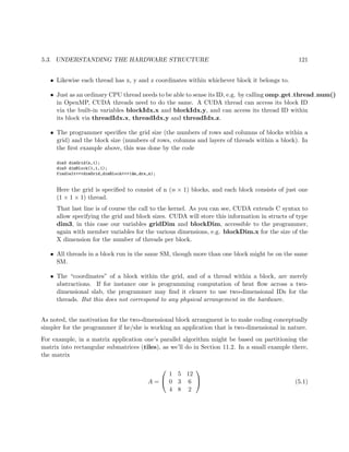
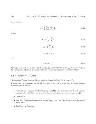
![5.6. HARDWARE REQUIREMENTS, INSTALLATION, COMPILATION, DEBUGGING 125
Download the CUDA toolkit from NVIDIA. Just plug “CUDA download” into a Web search engine
to find the site. Install as directed.
You’ll need to set your search and library paths to include the CUDA bin and lib directories.
To compile x.cu (and yes, use the .cu suffix), type
$ nvcc -g -G x.cu
The -g -G options are for setting up debugging, the first for host code, the second for device code.
You may also need to specify
-I/your_CUDA_include_path
to pick up the file cuda.h. Run the code as you normally would.
You may need to take special action to set your library path properly. For example, on Linux
machines, set the environment variable LD LIBRARY PATH to include the CUDA library.
To determine the limits, e.g. maximum number of threads, for your device, use code like this:
cudaDeviceProp Props;
cudaGetDeviceProperties(&Props,0);
The 0 is for device 0, assuming you only have one device. The return value of cudaGetDevice-
Properties() is a complex C struct whose components are listed at http://developer.download.
nvidia.com/compute/cuda/2_3/toolkit/docs/online/group__CUDART__DEVICE_g5aa4f47938af8276f08074d0
html.
Here’s a simple program to check some of the properties of device 0:
1 #include <cuda . h>
2 #include <s t d i o . h>
3
4 int main ()
5 {
6 cudaDeviceProp Props ;
7 cudaGetDeviceProperties ( &Props , 0 ) ;
8
9 p r i n t f (” shared mem: %d)n” , Props . sharedMemPerBlock ) ;
10 p r i n t f (”max threads / block : %dn” , Props . maxThreadsPerBlock ) ;
11 p r i n t f (”max blocks : %dn” , Props . maxGridSize [ 0 ] ) ;
12 p r i n t f (” t o t a l Const mem: %dn” , Props . totalConstMem ) ;
13 }](https://image.slidesharecdn.com/matloff-programmingonparallelmachines-2013-150626072019-lva1-app6892/85/Matloff-programming-on-parallel_machines-2013-145-320.jpg)
![5.7. EXAMPLE: IMPROVING THE ROW SUMS PROGRAM 127
17 sum = 0;
18 f o r (k = 0; k < n ; k++)
19 sum += m[ t o p o f c o l+k∗n ] ;
20 cs [ col ] = sum ;
21 }
22 }
23
24 int main ( int argc , char ∗∗ argv )
25 {
26 int n = a t oi ( argv [ 1 ] ) ; // number of matrix c o l s / c o l s
27 int ∗hm, // host matrix
28 ∗ hcs ; // host colsums
29 int msize = n ∗ n ∗ s i z e o f ( int ) ; // s i z e of matrix in bytes
30 // a l l o c a t e space f o r host matrix
31 hm = ( int ∗) malloc ( msize ) ;
32 // as a test , f i l l matrix with consecutive i n t e g e r s
33 int t = 0 , i , j ;
34 f o r ( i = 0; i < n ; i++) {
35 f o r ( j = 0; j < n ; j++) {
36 hm[ i ∗n+j ] = t++;
37 }
38 }
39 int c s s i z e = n ∗ s i z e o f ( int ) ;
40 hcs = ( int ∗) malloc ( c s s i z e ) ;
41 f i n d 1 e l t (hm, hcs , n ) ;
42 i f (n < 10) f o r ( i =0; i<n ; i++) p r i n t f (”%dn” , hcs [ i ] ) ;
43 // clean up
44 f r e e (hm) ;
45 f r e e ( hcs ) ;
46 }
How fast does this non-CUDA version run?
pc5:~/CUDA% time csc 20000
61.110u 1.719s 1:02.86 99.9% 0+0k 0+0io 0pf+0w
Very impressive! No wonder people talk of CUDA in terms like “a supercomputer on our desktop.”
And remember, this includes the time to copy the matrix from the host to the device (and to
copy the output array back). And we didn’t even try to optimize thread configuration, memory
coalescing and bank usage, making good use of memory hierarchy, etc.2
On the other hand, remember that this is an “embarrassingly parallel” application, and in many
applications we may have to settle for a much more modest increase, and work harder to get it.
2
Neither has the CPU-only version of the program been optimized. As pointed out by Bill Hsu, the row-major
version of that program should run faster than the column-major one, due to cache consideration.](https://image.slidesharecdn.com/matloff-programmingonparallelmachines-2013-150626072019-lva1-app6892/85/Matloff-programming-on-parallel_machines-2013-147-320.jpg)
![128 CHAPTER 5. INTRODUCTION TO GPU PROGRAMMING WITH CUDA
5.8 Example: Finding the Mean Number of Mutual Outlinks
As in Sections 2.4.3 and 4.12, consider a network graph of some kind, such as Web links. For any
two vertices, say any two Web sites, we might be interested in mutual outlinks, i.e. outbound links
that are common to two Web sites. The CUDA code below finds the mean number of mutual
outlinks, among all pairs of sites in a set of Web sites.
1 #include <cuda . h>
2 #include <s t d i o . h>
3
4 // CUDA example : f i n d s mean number of mutual outlinks , among a l l p a ir s
5 // of Web s i t e s in our set ; in checking a l l ( i , j ) pairs , thread k w i l l
6 // handle a l l i such that i mod totth = k , where totth i s the number of
7 // threads
8
9 // procpairs () processes a l l p a i r s f o r a given thread
10 g l o b a l void procpairs ( int ∗m, int ∗ tot , int n)
11 { int totth = gridDim . x ∗ blockDim . x , // t o t a l number of threads
12 me = blockIdx . x ∗ blockDim . x + threadIdx . x ; // my thread number
13 int i , j , k , sum = 0;
14 f o r ( i = me; i < n ; i += totth ) { // do various rows i
15 f o r ( j = i +1; j < n ; j++) { // do a l l rows j > i
16 f o r (k = 0; k < n ; k++)
17 sum += m[ n∗ i+k ] ∗ m[ n∗ j+k ] ;
18 }
19 }
20 atomicAdd ( tot , sum ) ;
21 }
22
23 int main ( int argc , char ∗∗ argv )
24 { int n = a t oi ( argv [ 1 ] ) , // number of v e r t i c e s
25 nblk = a to i ( argv [ 2 ] ) ; // number of blocks
26 int ∗hm, // host matrix
27 ∗dm, // device matrix
28 htot , // host grand t o t a l
29 ∗ dtot ; // device grand t o t a l
30 int msize = n ∗ n ∗ s i z e o f ( int ) ; // s i z e of matrix in bytes
31 // a l l o c a t e space f o r host matrix
32 hm = ( int ∗) malloc ( msize ) ;
33 // as a test , f i l l matrix with random 1 s and 0 s
34 int i , j ;
35 f o r ( i = 0; i < n ; i++) {
36 hm[ n∗ i+i ] = 0;
37 f o r ( j = 0; j < n ; j++) {
38 i f ( j != i ) hm[ i ∗n+j ] = rand () % 2;
39 }
40 }
41 // a l l o c a t e space f o r device matrix
42 cudaMalloc (( void ∗∗)&dm, msize ) ;](https://image.slidesharecdn.com/matloff-programmingonparallelmachines-2013-150626072019-lva1-app6892/85/Matloff-programming-on-parallel_machines-2013-148-320.jpg)
![5.9. EXAMPLE: FINDING PRIME NUMBERS 129
43 // copy host matrix to device matrix
44 cudaMemcpy(dm,hm, msize , cudaMemcpyHostToDevice ) ;
45 htot = 0;
46 // set up device t o t a l and i n i t i a l i z e i t
47 cudaMalloc (( void ∗∗)&dtot , s i z e o f ( int ) ) ;
48 cudaMemcpy( dtot ,&htot , s i z e o f ( int ) , cudaMemcpyHostToDevice ) ;
49 // set up parameters f o r threads structure
50 dim3 dimGrid ( nblk , 1 ) ;
51 dim3 dimBlock (192 ,1 ,1);
52 // invoke the kernel
53 procpairs <<<dimGrid , dimBlock>>>(dm, dtot , n ) ;
54 // wait f o r kernel to f i n i s h
55 cudaThreadSynchronize ( ) ;
56 // copy t o t a l from device to host
57 cudaMemcpy(&htot , dtot , s i z e o f ( int ) , cudaMemcpyDeviceToHost ) ;
58 // check r e s u l t s
59 i f (n <= 15) {
60 f o r ( i = 0; i < n ; i++) {
61 f o r ( j = 0; j < n ; j++)
62 p r i n t f (”%d ” ,hm[ n∗ i+j ] ) ;
63 p r i n t f (”n ” ) ;
64 }
65 }
66 p r i n t f (”mean = %f n” , htot / f l o a t (( n∗(n −1))/2));
67 // clean up
68 f r e e (hm) ;
69 cudaFree (dm) ;
70 cudaFree ( dtot ) ;
71 }
Again we’ve used the method in Section 2.4.3 to partition the various pairs (i,j) to the different
threads. Note the use of atomicAdd().
The above code is hardly optimal. The reader is encouraged to find improvements.
5.9 Example: Finding Prime Numbers
The code below finds all the prime numbers from 2 to n.
1 #include <s t d i o . h>
2 #include <s t d l i b . h>
3 #include <cuda . h>
4
5 // CUDA example : i l l u s t r a t i o n of shared memory a l l o c a t i o n at run time ;
6 // f i n d s primes using c l a s s i c a l Sieve of Erathosthenes : make l i s t of
7 // numbers 2 to n , then cross out a l l multiples of 2 ( but not 2 i t s e l f ) ,
8 // then a l l multiples of 3 , etc . ; whatever i s l e f t over i s prime ; in our](https://image.slidesharecdn.com/matloff-programmingonparallelmachines-2013-150626072019-lva1-app6892/85/Matloff-programming-on-parallel_machines-2013-149-320.jpg)
![130 CHAPTER 5. INTRODUCTION TO GPU PROGRAMMING WITH CUDA
9 // array , 1 w i l l mean ”not crossed out” and 0 w i l l mean ” crossed out”
10
11 // IMPORTANT NOTE: uses shared memory , in a s i n g l e block , without
12 // rotating parts of array in and out of shared memory ; thus limited to
13 // n <= 4000 i f have 16K shared memory
14
15 // i n i t i a l i z e sprimes , 1 s f o r the odds , 0 s f o r the evens ; see s i e v e ()
16 // f o r the nature of the arguments
17 d e v i c e void i n i t s p ( int ∗ sprimes , int n , int nth , int me)
18 {
19 int chunk , s t ar t se ts p , endsetsp , val , i ;
20 sprimes [ 2 ] = 1;
21 // determine sprimes chunk f o r t h i s thread to i n i t
22 chunk = (n−1) / nth ;
23 s t a r t s e t s p = 2 + me∗chunk ;
24 i f (me < nth −1) endsetsp = s t a r t s e t s p + chunk − 1;
25 e l s e endsetsp = n ;
26 // now do the i n i t
27 val = s t a r t s e t s p % 2;
28 f o r ( i = s t a r t s e t s p ; i <= endsetsp ; i++) {
29 sprimes [ i ] = val ;
30 val = 1 − val ;
31 }
32 // make sure sprimes up to date f o r a l l
33 syncthreads ( ) ;
34 }
35
36 // copy sprimes back to device global memory ; see s i e v e () f o r the nature
37 // of the arguments
38 d e v i c e void cpytoglb ( int ∗dprimes , int ∗ sprimes , int n , int nth , int me)
39 {
40 int startcpy , endcpy , chunk , i ;
41 chunk = (n−1) / nth ;
42 startcpy = 2 + me∗chunk ;
43 i f (me < nth −1) endcpy = startcpy + chunk − 1;
44 e l s e endcpy = n ;
45 f o r ( i = startcpy ; i <= endcpy ; i++) dprimes [ i ] = sprimes [ i ] ;
46 syncthreads ( ) ;
47 }
48
49 // f i n d s primes from 2 to n , s t o r i n g the information in dprimes , with
50 // dprimes [ i ] being 1 i f i i s prime , 0 i f composite ; nth i s the number
51 // of threads ( threadDim somehow not recognized )
52 g l o b a l void s i e v e ( int ∗dprimes , int n , int nth )
53 {
54 extern s h a r e d int sprimes [ ] ;
55 int me = threadIdx . x ;
56 int nth1 = nth − 1;
57 // i n i t i a l i z e sprimes array , 1 s f o r odds , 0 f o r evens
58 i n i t s p ( sprimes , n , nth ,me ) ;](https://image.slidesharecdn.com/matloff-programmingonparallelmachines-2013-150626072019-lva1-app6892/85/Matloff-programming-on-parallel_machines-2013-150-320.jpg)
![5.9. EXAMPLE: FINDING PRIME NUMBERS 131
59 // ” cross out” multiples of various numbers m, with each thread doing
60 // a chunk of m’ s ; always check f i r s t to determine whether m has
61 // already been found to be composite ; f i n i s h when m∗m > n
62 int maxmult ,m, startmult , endmult , chunk , i ;
63 f o r (m = 3; m∗m <= n ; m++) {
64 i f ( sprimes [m] != 0) {
65 // find l a r g e s t multiple of m that i s <= n
66 maxmult = n / m;
67 // now p a r t i t i o n 2 , 3 , . . . , maxmult among the threads
68 chunk = (maxmult − 1) / nth ;
69 startmult = 2 + me∗chunk ;
70 i f (me < nth1 ) endmult = startmult + chunk − 1;
71 e l s e endmult = maxmult ;
72 }
73 // OK, cross out my chunk
74 f o r ( i = startmult ; i <= endmult ; i++) sprimes [ i ∗m] = 0;
75 }
76 syncthreads ( ) ;
77 // copy back to device global memory f o r return to host
78 cpytoglb ( dprimes , sprimes , n , nth ,me ) ;
79 }
80
81 int main ( int argc , char ∗∗ argv )
82 {
83 int n = a t oi ( argv [ 1 ] ) , // w i l l find primes among 1 , . . . , n
84 nth = a t oi ( argv [ 2 ] ) ; // number of threads
85 int ∗hprimes , // host primes l i s t
86 ∗dprimes ; // device primes l i s t
87 int p s i z e = (n+1) ∗ s i z e o f ( int ) ; // s i z e of primes l i s t s in bytes
88 // a l l o c a t e space f o r host l i s t
89 hprimes = ( int ∗) malloc ( p s i z e ) ;
90 // a l l o c a t e space f o r device l i s t
91 cudaMalloc (( void ∗∗)&dprimes , p s i z e ) ;
92 dim3 dimGrid ( 1 , 1 ) ;
93 dim3 dimBlock ( nth , 1 , 1 ) ;
94 // invoke the kernel , including a request to a l l o c a t e shared memory
95 sieve <<<dimGrid , dimBlock , psize >>>(dprimes , n , nth ) ;
96 // check whether we asked f o r too much shared memory
97 cudaError t err = cudaGetLastError ( ) ;
98 i f ( err != cudaSuccess ) p r i n t f (”%s n” , cudaGetErrorString ( err ) ) ;
99 // wait f o r kernel to f i n i s h
100 cudaThreadSynchronize ( ) ;
101 // copy l i s t from device to host
102 cudaMemcpy( hprimes , dprimes , psize , cudaMemcpyDeviceToHost ) ;
103 // check r e s u l t s
104 i f (n <= 1000) f o r ( int i =2; i<=n ; i++)
105 i f ( hprimes [ i ] == 1) p r i n t f (”%dn” , i ) ;
106 // clean up
107 f r e e ( hprimes ) ;
108 cudaFree ( dprimes ) ;](https://image.slidesharecdn.com/matloff-programmingonparallelmachines-2013-150626072019-lva1-app6892/85/Matloff-programming-on-parallel_machines-2013-151-320.jpg)
![5.11. EXAMPLE: TRANSFORMING AN ADJACENCY MATRIX 133
which together with the 4 found by thread 0 makes 6. Thus thread 2 must add 6 to each of its
elements, i.e. add 6 to (3,3), yielding (9,9). The case of thread 3 is similar.
Below is code for the special case of a single block:
1 // f o r t h i s simple i l l u s t r a t i o n , i t i s assumed that the code runs in
2 // j u s t one block , and that the number of threads evenly divides n
3
4 #include <cuda . h>
5 #include <s t d i o . h>
6
7 g l o b a l void cumulker ( int ∗dx , int n)
8 {
9 int me = threadIdx . x ;
10 int c s i z e = n / blockDim . x ;
11 int s t a r t = me ∗ c s i z e ;
12 int i , j , base ;
13 f o r ( i = 1; i < c s i z e ; i++) {
14 j = s t a r t + i ;
15 dx [ j ] = dx [ j −1] + dx [ j ] ;
16 }
17 syncthreads ( ) ;
18 i f (me > 0) {
19 base = 0;
20 f o r ( j = 0; j < me; j++)
21 base += dx [ ( j +1)∗ csize −1];
22 }
23 syncthreads ( ) ;
24 i f (me > 0) {
25 f o r ( i = s t a r t ; i < s t a r t + c s i z e ; i++)
26 dx [ i ] += base ;
27 }
28 }
5.11 Example: Transforming an Adjacency Matrix
Here is a CUDA version of the code in Section 4.13.
1 // CUDA example
2
3 // takes a graph adjacency matrix f o r a directed graph , and converts i t
4 // to a 2−column matrix of p a i r s ( i , j ) , meaning an edge from vertex i to
5 // vertex j ; the output matrix must be in l e x i c o g r a p h i c a l order
6
7 // not claimed e f f i c i e n t , e i t h e r in speed or in memory usage
8
9 #include <cuda . h>
10 #include <s t d i o . h>](https://image.slidesharecdn.com/matloff-programmingonparallelmachines-2013-150626072019-lva1-app6892/85/Matloff-programming-on-parallel_machines-2013-153-320.jpg)
![134 CHAPTER 5. INTRODUCTION TO GPU PROGRAMMING WITH CUDA
11
12 // needs −l r t l i n k f l a g f o r C++
13 #include <time . h>
14 f l o a t t i m e d i f f ( s t r u c t timespec t1 , s t r u c t timespec t2 )
15 { i f ( t1 . tv nsec > t2 . tv nsec ) {
16 t2 . t v s e c −= 1;
17 t2 . tv nsec += 1000000000;
18 }
19 return t2 . tv sec −t1 . t v s e c + 0.000000001 ∗ ( t2 . tv nsec −t1 . tv nsec ) ;
20 }
21
22
23 // kernel transgraph () does t h i s work
24 // arguments :
25 // adjm : the adjacency matrix (NOT assumed symmetric ) , 1 f o r edge , 0
26 // otherwise ; note : matrix i s overwritten by the function
27 // n : number of rows and columns of adjm
28 // adjmout : output matrix
29 // nout : number of rows in adjmout
30
31 g l o b a l void tgkernel1 ( int ∗dadjm , int n , int ∗ dcounts )
32 { int tot1s , j ;
33 int me = blockDim . x ∗ blockIdx . x + threadIdx . x ;
34 tot1s = 0;
35 f o r ( j = 0; j < n ; j++) {
36 i f ( dadjm [ n∗me+j ] == 1) {
37 dadjm [ n∗me+tot1s++] = j ;
38 }
39 dcounts [me] = tot1s ;
40 }
41 }
42
43 g l o b a l void tgkernel2 ( int ∗dadjm , int n ,
44 int ∗dcounts , int ∗ dstarts , int ∗doutm)
45 { int outrow , num1si , j ;
46 // int me = threadIdx . x ;
47 int me = blockDim . x ∗ blockIdx . x + threadIdx . x ;
48 // f i l l in t h i s thread ’ s portion of doutm
49 outrow = d s t a r t s [me ] ;
50 num1si = dcounts [me ] ;
51 i f ( num1si > 0) {
52 f o r ( j = 0; j < num1si ; j++) {
53 doutm [2∗ outrow+2∗ j ] = me;
54 doutm [2∗ outrow+2∗ j +1] = dadjm [ n∗me+j ] ;
55 }
56 }
57 }
58
59 // r e p l a c e s counts by cumulative counts
60 void cumulcounts ( int ∗c , int ∗s , int n)](https://image.slidesharecdn.com/matloff-programmingonparallelmachines-2013-150626072019-lva1-app6892/85/Matloff-programming-on-parallel_machines-2013-154-320.jpg)
![5.11. EXAMPLE: TRANSFORMING AN ADJACENCY MATRIX 135
61 { int i ;
62 s [ 0 ] = 0;
63 f o r ( i = 1; i < n ; i++) {
64 s [ i ] = s [ i −1] + c [ i −1];
65 }
66 }
67
68 int ∗ transgraph ( int ∗hadjm , int n , int ∗nout , int gsize , int b s i z e )
69 { int ∗dadjm ; // device adjacency matrix
70 int ∗houtm ; // host output matrix
71 int ∗doutm ; // device output matrix
72 int ∗ hcounts ; // host counts vector
73 int ∗ dcounts ; // device counts vector
74 int ∗ h s t a r t s ; // host s t a r t s vector
75 int ∗ d s t a r t s ; // device s t a r t s vector
76 hcounts = ( int ∗) malloc (n∗ s i z e o f ( int ) ) ;
77 h s t a r t s = ( int ∗) malloc (n∗ s i z e o f ( int ) ) ;
78 cudaMalloc (( void ∗∗)&dadjm , n∗n∗ s i z e o f ( int ) ) ;
79 cudaMalloc (( void ∗∗)&dcounts , n∗ s i z e o f ( int ) ) ;
80 cudaMalloc (( void ∗∗)& dstarts , n∗ s i z e o f ( int ) ) ;
81 houtm = ( int ∗) malloc (n∗n∗ s i z e o f ( int ) ) ;
82 cudaMalloc (( void ∗∗)&doutm , n∗n∗ s i z e o f ( int ) ) ;
83 cudaMemcpy(dadjm , hadjm , n∗n∗ s i z e o f ( int ) , cudaMemcpyHostToDevice ) ;
84 dim3 dimGrid ( gsize , 1 ) ;
85 dim3 dimBlock ( bsize , 1 , 1 ) ;
86 // c a l c u l a t e counts and s t a r t s f i r s t
87 tgkernel1 <<<dimGrid , dimBlock>>>(dadjm , n , dcounts ) ;
88 // cudaMemcpy(hadjm , dadjm , n∗n∗ s i z e o f ( int ) , cudaMemcpyDeviceToHost ) ;
89 cudaMemcpy( hcounts , dcounts , n∗ s i z e o f ( int ) , cudaMemcpyDeviceToHost ) ;
90 cumulcounts ( hcounts , hstarts , n ) ;
91 ∗nout = h s t a r t s [ n−1] + hcounts [ n−1];
92 cudaMemcpy( dstarts , hstarts , n∗ s i z e o f ( int ) , cudaMemcpyHostToDevice ) ;
93 tgkernel2 <<<dimGrid , dimBlock>>>(dadjm , n , dcounts , dstarts , doutm ) ;
94 cudaMemcpy(houtm , doutm ,2∗(∗ nout )∗ s i z e o f ( int ) , cudaMemcpyDeviceToHost ) ;
95 f r e e ( hcounts ) ;
96 f r e e ( h s t a r t s ) ;
97 cudaFree ( dadjm ) ;
98 cudaFree ( dcounts ) ;
99 cudaFree ( d s t a r t s ) ;
100 return houtm ;
101 }
102
103 int main ( int argc , char ∗∗ argv )
104 { int i , j ;
105 int ∗adjm ; // host adjacency matrix
106 int ∗outm ; // host output matrix
107 int n = at o i ( argv [ 1 ] ) ;
108 int g s i z e = a t o i ( argv [ 2 ] ) ;
109 int b s i z e = a t o i ( argv [ 3 ] ) ;
110 int nout ;](https://image.slidesharecdn.com/matloff-programmingonparallelmachines-2013-150626072019-lva1-app6892/85/Matloff-programming-on-parallel_machines-2013-155-320.jpg)
![136 CHAPTER 5. INTRODUCTION TO GPU PROGRAMMING WITH CUDA
111 adjm = ( int ∗) malloc (n∗n∗ s i z e o f ( int ) ) ;
112 f o r ( i = 0; i < n ; i++)
113 f o r ( j = 0; j < n ; j++)
114 i f ( i == j ) adjm [ n∗ i+j ] = 0;
115 e l s e adjm [ n∗ i+j ] = rand () % 2;
116 i f (n < 10) {
117 p r i n t f (” adjacency matrix : n ” ) ;
118 f o r ( i = 0; i < n ; i++) {
119 f o r ( j = 0; j < n ; j++) p r i n t f (”%d ” , adjm [ n∗ i+j ] ) ;
120 p r i n t f (”n ” ) ;
121 }
122 }
123
124 s t r u c t timespec bgn , nd ;
125 clock gettime (CLOCK REALTIME, &bgn ) ;
126
127 outm = transgraph (adjm , n,&nout , gsize , b s i z e ) ;
128 p r i n t f (”num rows in out matrix = %dn” , nout ) ;
129 i f ( nout < 50) {
130 p r i n t f (” out matrix : n ” ) ;
131 f o r ( i = 0; i < nout ; i++)
132 p r i n t f (”%d %dn” ,outm [2∗ i ] , outm [2∗ i +1]);
133 }
134
135 clock gettime (CLOCK REALTIME, &nd ) ;
136 p r i n t f (”% f n” , t i m e d i f f (bgn , nd ) ) ;
137 }
5.12 Error Checking
Every CUDA call (except for kernel invocations) returns an error code of type cudaError t. One
can view the nature of the error by calling cudaGetErrorString() and printing its output.
For kernel invocations, one can call cudaGetLastError(), which does what its name implies. A
call would typically have the form
cudaError_t err = cudaGetLastError();
if(err != cudaSuccess) printf("%sn",cudaGetErrorString(err));
You may also wish to cutilSafeCall(), which is used by wrapping your regular CUDA call. It
automatically prints out error messages as above.
Each CUBLAS call returns a potential error code, of type cublasStatus, not checked here.](https://image.slidesharecdn.com/matloff-programmingonparallelmachines-2013-150626072019-lva1-app6892/85/Matloff-programming-on-parallel_machines-2013-156-320.jpg)
![5.13. LOOP UNROLLING 137
5.13 Loop Unrolling
Loop unrolling is an old technique used on uniprocessor machines to achieve speedup due to
branch elimination and the like. Branches make it difficult to do instruction or data prefetching,
so eliminating them may speed things up.
The CUDA compiler provides the programmer with the unroll pragma to request loop unrolling.
Here an n-iteration for loop is changed to k copies of the body of the loop, each working on about
n/k iterations. If n and k are known constant, GPU registers can be used to implement the unrolled
loop.
For example, the loop
for (i = 0; i < 2; i++ {
sum += x[i];
sum2 += x[i]*x[i];
}
could be unrolled to
sum += x[1];
sum2 += x[1]*x[1];
sum += x[2];
sum2 += x[2]*x[2];
Here n = k = 2. If x is local to this function, then unrolling will allow the compiler to store it in
a register, which could be a great performance enhancer.
The compiler will try to do loop unrolling even if the programmer doesn’t request it, but the
programmer can try to control things by using the pragma:
#pragma unroll k
suggest to the compiler a k-fold unrolling. Setting k = 1 will instruct the compiler not to unroll.
5.14 Short Vectors
In CUDA, there are types such as int4, char2 and so on, up to four elements each. So, an uint4
type is a set of four unsigned ints. These are called short vectors.
The key point is that a short vector can be treated as a single word in terms of memory access
and GPU instructions. It may be possible to reduce time by a factor of 4 by dividing arrays into
chunks of four contiguous words and making short vectors from them.](https://image.slidesharecdn.com/matloff-programmingonparallelmachines-2013-150626072019-lva1-app6892/85/Matloff-programming-on-parallel_machines-2013-157-320.jpg)
![5.16. CUDA FROM A HIGHER LEVEL 139
5.16.1.1 Example: Row Sums Once Again
Below is an example RowSumsCB.c, the matrix row sums example again, this time using
CUBLAS. We can find the vector of row sums of the matrix A by post-multiplying A by a column
vector of all 1s.
I compiled the code by typing
gcc -g -I/usr/local/cuda/include -L/usr/local/cuda/lib RowSumsCB.c -lcublas -lcudart
You should modify for your own CUDA locations accordingly. Users who merely wish to use
CUBLAS will find the above more convenient, but if you are mixing CUDA and CUBLAS, you
would use nvcc:
nvcc -g -G RowSumsCB.c -lcublas
Here is the code:
1 #include <s t d i o . h>
2 #include <cublas . h> // required include
3
4 int main ( int argc , char ∗∗ argv )
5 {
6 int n = at o i ( argv [ 1 ] ) ; // number of matrix rows/ c o l s
7 f l o a t ∗hm, // host matrix
8 ∗hrs , // host rowsums vector
9 ∗ones , // 1 s vector f o r multiply
10 ∗dm, // device matrix
11 ∗ drs ; // device rowsums vector
12 // a l l o c a t e space on host
13 hm = ( f l o a t ∗) malloc (n∗n∗ s i z e o f ( f l o a t ) ) ;
14 hrs = ( f l o a t ∗) malloc (n∗ s i z e o f ( f l o a t ) ) ;
15 ones = ( f l o a t ∗) malloc (n∗ s i z e o f ( f l o a t ) ) ;
16 // as a test , f i l l hm with consecutive integers , but in column−major
17 // order f o r CUBLAS; also put 1 s in ones
18 int i , j ;
19 f l o a t t = 0 . 0 ;
20 f o r ( i = 0; i < n ; i++) {
21 ones [ i ] = 1 . 0 ;
22 f o r ( j = 0; j < n ; j++)
23 hm[ j ∗n+i ] = t++;
24 }
25 c u b l a s I n i t ( ) ; // required i n i t
26 // set up space on the device
27 cublasAlloc (n∗n , s i z e o f ( f l o a t ) , ( void ∗∗)&dm) ;
28 cublasAlloc (n , s i z e o f ( f l o a t ) , ( void ∗∗)& drs ) ;](https://image.slidesharecdn.com/matloff-programmingonparallelmachines-2013-150626072019-lva1-app6892/85/Matloff-programming-on-parallel_machines-2013-159-320.jpg)
![140 CHAPTER 5. INTRODUCTION TO GPU PROGRAMMING WITH CUDA
29 // copy data from host to device
30 cublasSetMatrix (n , n , s i z e o f ( f l o a t ) ,hm, n ,dm, n ) ;
31 cublasSetVector (n , s i z e o f ( f l o a t ) , ones , 1 , drs , 1 ) ;
32 // matrix times vector (”mv”)
33 cublasSgemv ( ’ n ’ , n , n , 1 . 0 ,dm, n , drs , 1 , 0 . 0 , drs , 1 ) ;
34 // copy r e s u l t back to host
35 cublasGetVector (n , s i z e o f ( f l o a t ) , drs , 1 , hrs , 1 ) ;
36 // check r e s u l t s
37 i f (n < 20) f o r ( i = 0; i < n ; i++) p r i n t f (”% f n” , hrs [ i ] ) ;
38 // clean up on device ( should c a l l f r e e () on host too )
39 cublasFree (dm) ;
40 cublasFree ( drs ) ;
41 cublasShutdown ( ) ;
42 }
As noted in the comments, CUBLAS assumes FORTRAN-style, i.e. column-major order, for
matrices.
Now that you know the basic format of CUDA calls, the CUBLAS versions will look similar. In
the call
cublasAlloc(n*n,sizeof(float),(void**)&dm);
for instance, we are allocating space on the device for an n x n matrix of floats.
The call
cublasSetMatrix(n,n,sizeof(float),hm,n,dm,n);
is slightly more complicated. Here we are saying that we are copying hm, an n x n matrix of floats
on the host, to dm on the host. The n arguments in the last and third-to-last positions again say
that the two matrices each have n dimensioned rows. This seems redundant, but this is needed in
cases of matrix tiling, where the number of rows of a tile would be less than the number of rows of
the matrix as a whole.
The 1s in the call
cublasSetVector(n,sizeof(float),ones,1,drs,1);
are needed for similar reasons. We are saying that in our source vector ones, for example, the
elements of interest are spaced 1 elements apart, i.e. they are contiguous. But if we wanted our
vector to be some row in a matrix with, say, 500 rows, the elements of any particular row of interest
would be spaced 500 elements apart, again keeping in mind that column-major order is assumed.
The actual matrix multiplication is done here:](https://image.slidesharecdn.com/matloff-programmingonparallelmachines-2013-150626072019-lva1-app6892/85/Matloff-programming-on-parallel_machines-2013-160-320.jpg)

![6.2. EXAMPLE: COUNTING THE NUMBER OF UNIQUE VALUES IN AN ARRAY 145
15 // match , 1 when they don ’ t
16 s t r u c t f i n d d i f f
17 {
18 d e v i c e int operator ( ) ( const int& x , const int&y)
19 { return x == y ? 0 : 1 ; }
20 };
21
22 int main ( void )
23 {
24 // generate t e s t data , 1000 random numbers , on the host , int type
25 thrust : : host vector <int> hv (1000);
26 thrust : : generate (hv . begin ( ) , hv . end ( ) , rand16 ) ;
27
28 // copy data to the device , creating a vector there
29 thrust : : device vector <int> dv = hv ;
30
31 // sort data on the device
32 thrust : : sort (dv . begin ( ) , dv . end ( ) ) ;
33
34 // create device vector to hold d i f f e r e n c e s , with length 1 l e s s than
35 // dv ’ s length
36 thrust : : device vector <int> d i f f s (dv . s i z e () −1);
37
38 // find the d i f f s ; note that the syntax i s f i n d d i f f ( ) , not f i n d d i f f
39 thrust : : transform (dv . begin ( ) , dv . end() −1 ,
40 dv . begin ()+1 , d i f f s . begin ( ) , f i n d d i f f ( ) ) ;
41
42 // count the 1s , by removing 0 s and checking new length
43 // ( or could use thrust : : count ( ) )
44 int n d i f f s = thrust : : reduce ( d i f f s . begin ( ) , d i f f s . end ( ) , ( int ) 0 ,
45 thrust : : plus<int >());
46 p r i n t f (”# d i s t i n c t : %dn” , n d i f f s +1);
47
48 // we ’ ve achieved our goal , but let ’ s do a l i t t l e more
49 // t r a n s f e r data back to host
50 thrust : : copy (dv . begin ( ) , dv . end ( ) , hv . begin ( ) ) ;
51
52 p r i n t f (” the sorted array : n ” ) ;
53 f o r ( int i = 0; i < 1000; i++) p r i n t f (”%dn” ,hv [ i ] ) ;
54
55 return 0;
56 }
After generating some random data on a host array hv, we copy it to the device, creating a vector
dv there. This code is certainly much simpler to write than slogging through calls to cudaMalloc()
and cudaMemcpy()!
The heart of the code is the call to thrust::transform(), which is used to implement step (b) in
our outline above. It performs a “map” operation as in functional programming, taking one or two](https://image.slidesharecdn.com/matloff-programmingonparallelmachines-2013-150626072019-lva1-app6892/85/Matloff-programming-on-parallel_machines-2013-165-320.jpg)
![148 CHAPTER 6. INTRODUCTION TO THRUST PROGRAMMING
6.3 Example: A Plain-C Wrapper for Thrust sort()
We may wish to wrap utility Thrust code in a function callable from a purely C/C++ program.
The code below does that for the Thrust sort function.
1 // d e f i n i t e l y needed
2 extern ”C” void t s o r t ( int ∗x , int ∗nx ) ;
3
4 #include <thrust / d evi ce ve cto r . h>
5 #include <thrust / sort . h>
6
7 // nx set up as pointer so can c a l l from R
8 void t s o r t ( int ∗x , int ∗nx)
9 { int n = ∗nx ;
10 // set up device vector and copy x to i t
11 thrust : : device vector <int> dx(x , x+n ) ;
12 // sort , then copy back to x
13 thrust : : sort (dx . begin ( ) , dx . end ( ) ) ;
14 thrust : : copy (dx . begin ( ) , dx . end ( ) , x ) ;
15 }
To compile in the CUDA case, run nvcc -c and then run gcc (or whatever) as usual, making sure
to link with the CUDA library. For instance,
nvcc −c SortForC . cu
gcc Main . c S∗o −L/ usr / l o c a l /cuda/ l i b −lcudart
Here’s an example:
1 // TestSort . cpp : i n t e r f a c e to Thrust sort from non−CUDA c a l l e r s
2
3 #include <s t d i o . h>
4
5 extern ”C” void t s o r t ( int ∗x , int ∗nx ) ;
6
7 // t e s t
8 int main ()
9 { int x [ 5 ] = {12 ,13 ,5 ,8 ,88};
10 int n=5,∗nx ; nx = &n ;
11 int i ;
12 t s o r t (x , nx ) ;
13 f o r ( i = 0; i < 5; i++) p r i n t f (”%dn” ,x [ i ] ) ;
14 }
Compile and run for the OpenMP case:
g++ −g −mcmodel=medium −fopenmp −lgomp
−DTHRUST DEVICE BACKEND=THRUST DEVICE BACKEND OMP
−I /home/ matloff /Thrust SortForC . cpp −o sort . o −c](https://image.slidesharecdn.com/matloff-programmingonparallelmachines-2013-150626072019-lva1-app6892/85/Matloff-programming-on-parallel_machines-2013-168-320.jpg)
![150 CHAPTER 6. INTRODUCTION TO THRUST PROGRAMMING
22 { return i != 0 && ( i % increm ) == 0;
23 }
24 };
25
26 // t e s t
27 int main ( int argc , char ∗∗ argv )
28 { int x [ 1 5 ] = {6 ,12 ,5 ,13 ,3 ,5 ,4 ,5 ,8 ,88 ,1 ,11 ,9 ,22 ,168};
29 int n=15;
30 thrust : : device vector <int> dx(x , x+n ) ;
31 thrust : : sort (dx . begin ( ) , dx . end ( ) ) ;
32 thrust : : device vector <int> seq (n ) ;
33 thrust : : sequence ( seq . begin ( ) , seq . end ( ) , 0 ) ;
34 thrust : : device vector <int> out (n ) ;
35 int inc r = a t oi ( argv [ 1 ] ) ; // k
36 // f o r each i in seq , c a l l ismultk () on t h i s i , and i f get a true
37 // result , put dx [ i ] into out
38 thrust : : device vector <int >:: i t e r a t o r newend =
39 thrust : : c o p y i f (dx . begin ( ) , dx . end ( ) , seq . begin ( ) , out . begin ( ) ,
40 ismultk ( in cr ) ) ;
41 thrust : : copy ( out . begin ( ) , newend ,
42 std : : ostream iterator <int >(std : : cout , ” ” ) ) ;
43 std : : cout << ”n ”;
44 }
The sequence() function simply generates an array consisting of 0,1,2,...,n-1.
Our functor here is a little more advanced than the one we saw earlier. It now has an argument,
which is incr in the case of our call,
thrust : : c o p y i f (dx . begin ( ) , dx . end ( ) , seq , out , ismultk ( i ncr ) ) ;
That is then used to set a member variable in the struct:
const int increm ; // k in above comments
ismultk ( int increm ) : increm ( increm ) {}
This is in a sense the second, though nonexplicit, argument to our calls to ismultk(). For example,
in our call,
thrust : : c o p y i f (hx . begin ( ) , hx . end ( ) , seq , out , ismultk ( i ncr ) ) ;
the function designated by operator within the ismultk struct will be called individually on each
element in hx, each one playing role of i in
bool operator ( ) ( const int i )
{ return i != 0 && ( i % increm ) == 0;
}
Since this code references increm, the value incr in our call above is used as well. The variable
increm acts as a “global” variable to all the actions of the operator.](https://image.slidesharecdn.com/matloff-programmingonparallelmachines-2013-150626072019-lva1-app6892/85/Matloff-programming-on-parallel_machines-2013-170-320.jpg)
![6.5. MIXING THRUST AND CUDA CODE 151
6.5 Mixing Thrust and CUDA Code
In order to mix Thrust and CUDA code, Thrust has the function thrust::raw pointer cast() to
convert from a Thrust device pointer type to a CUDA device pointer type, and has thrust::device ptr
to convert in the other direction.
In our example in Section 6.6, we convert from Thrust to an ordinary address on the device:
int ∗wd;
. . .
wd = thrust : : raw pointer cast (&w [ 0 ] ) ;
. . .
{ i f ( i != 0 && ( i % increm ) == 0) wd[ i ] = 2 ∗ wd[ i ] ;
In the other direction, say we start with a CUDA pointer, and want to use it in Thrust. We might
have something like
int ∗dz ;
. . .
cudaMalloc(&dz ,100∗ s i z e o f ( int ) ) ;
. . .
thrust : : device ptr <int> tz ( dz ) ;
. . .
int k = thrust : : reduce ( tz , tz +100, ( int ) 0 , thrust : : plus<int >());
6.6 Example: Doubling Every kth
Element of an Array
Let’s adapt the code from the last section in order to illustrate another technique.
Suppose instead of copying every kth element of an array (after this first one), we wish to merely
double each such element. There are various ways we could do this, but here we’ll use an approach
that shows another way we can use functors.
1 // double every k−th element in given array ; k obtained from command
2 // l i n e
3
4 #include <s t d i o . h>
5
6 #include <thrust / d evi ce ve cto r . h>
7 #include <thrust / sequence . h>
8 #include <thrust /remove . h> // f o r c o p y i f ()
9
10 // functor
11 s t r u c t ismultk
12 {
13 const int increm ; // k in above comments](https://image.slidesharecdn.com/matloff-programmingonparallelmachines-2013-150626072019-lva1-app6892/85/Matloff-programming-on-parallel_machines-2013-171-320.jpg)
![152 CHAPTER 6. INTRODUCTION TO THRUST PROGRAMMING
14 const thrust : : device vector <int >:: i t e r a t o r w; // ” pointer ” to our array
15 int ∗wd;
16 // get ” pointer ,” k
17 ismultk ( thrust : : device vector <int >:: i t e r a t o r w , int increm ) :
18 w( w ) , increm ( increm ) {
19 wd = thrust : : raw pointer cast (&w [ 0 ] ) ;
20 }
21 d e v i c e
22 bool operator ( ) ( const int i ) // bool i s phony , but void doesn ’ t work
23 { i f ( i != 0 && ( i % increm ) == 0) wd[ i ] = 2 ∗ wd[ i ] ;
24 }
25 };
26
27 // t e s t
28 int main ( int argc , char ∗∗ argv )
29 { // t e s t case :
30 int x [ 1 5 ] = {6 ,12 ,5 ,13 ,3 ,5 ,4 ,5 ,8 ,88 ,1 ,11 ,9 ,22 ,168};
31 int n=15;
32 thrust : : device vector <int> dx(x , x+n ) ;
33 thrust : : device vector <int> seq (n ) ;
34 thrust : : sequence ( seq . begin ( ) , seq . end ( ) , 0 ) ;
35 thrust : : device vector <int> out (n ) ;
36 int inc r = a t oi ( argv [ 1 ] ) ; // k
37 // f o r each i in seq , c a l l ismultk () on t h i s i , and i f get a true
38 // result , put 0 in dx [ i ]
39 thrust : : c o p y i f (dx . begin ( ) , dx . end ( ) , seq . begin ( ) , out . begin ( ) ,
40 ismultk (dx . begin ( ) , in cr ) ) ;
41 // did i t work?
42 thrust : : copy (dx . begin ( ) , dx . end ( ) ,
43 std : : ostream iterator <int >(std : : cout , ” ” ) ) ;
44 std : : cout << ”n ”;
45 }
Our functor here is quite different from before.
First, one of the functor’s arguments is an iterator, rather than a simple type like int. This is really
just like passing an array pointer to an ordinary C function.
Second, we’ve converted that iterator to a simple device array
1 const thrust : : device vector <int >:: i t e r a t o r w; // ” pointer ” to our array
2 int ∗wd;
3 . . .
4 wd = thrust : : raw pointer cast (&w [ 0 ] ) ;
Our call to copy if() doesn’t actually do any copying. We are exploiting the “if” in “copy if,” not
the “copy.”](https://image.slidesharecdn.com/matloff-programmingonparallelmachines-2013-150626072019-lva1-app6892/85/Matloff-programming-on-parallel_machines-2013-172-320.jpg)
![6.7. SCATTER AND GATHER OPERATIONS 153
6.7 Scatter and Gather Operations
These basically act as permuters; see the comments in the following small examples.
scatter:
1 // i l l u s t r a t i o n of thrust : : s c a t t e r ( ) ; permutes an array according to a
2 // map array
3
4 #include <s t d i o . h>
5 #include <thrust / d evi ce ve cto r . h>
6 #include <thrust / s c a t t e r . h>
7
8 int main ()
9 { int x [ 5 ] = {12 ,13 ,5 ,8 ,88};
10 int n=5;
11 thrust : : device vector <int> dx(x , x+n ) ;
12 // a l l o c a t e map vector
13 thrust : : device vector <int> dm(n ) ;
14 // a l l o c a t e vector f o r output of gather
15 thrust : : device vector <int> hdst (n ) ;
16 // example map
17 int m[ 5 ] = {3 ,2 ,4 ,1 ,0};
18 thrust : : copy (m,m+n ,dm. begin ( ) ) ;
19 thrust : : s c a t t e r (dx . begin ( ) , dx . end ( ) ,dm. begin ( ) , ddst . begin ( ) ) ;
20 // the o r i g i n a l x [ 0 ] should now be at p o s i t i o n 3 , the o r i g i n a l x [ 1 ]
21 // now at p o s i t i o n 2 , etc . , i . e . 88 ,8 ,13 ,12; ,5 check i t :
22 thrust : : copy ( ddst . begin ( ) , ddst . end ( ) ,
23 std : : ostream iterator <int >(std : : cout , ” ” ) ) ;
24 std : : cout << ”n ”;
25 }
gather():
1 // i l l u s t r a t i o n s of thrust : : gather ( ) ; permutes an array according to a
2 // map array
3
4 #include <s t d i o . h>
5 #include <thrust / d evi ce ve cto r . h>
6 #include <thrust / gather . h>
7
8 int main ()
9 { int x [ 5 ] = {12 ,13 ,5 ,8 ,88};
10 int n=5;
11 thrust : : device vector <int> dx(x , x+n ) ;
12 // a l l o c a t e map vector
13 thrust : : device vector <int> dm(n ) ;
14 // a l l o c a t e vector f o r output of gather
15 thrust : : device vector <int> ddst (n ) ;
16 // example map](https://image.slidesharecdn.com/matloff-programmingonparallelmachines-2013-150626072019-lva1-app6892/85/Matloff-programming-on-parallel_machines-2013-173-320.jpg)
![154 CHAPTER 6. INTRODUCTION TO THRUST PROGRAMMING
17 int m[ 5 ] = {3 ,2 ,4 ,1 ,0};
18 thrust : : copy (m,m+n ,dm. begin ( ) ) ;
19 thrust : : gather (dm. begin ( ) ,dm. end ( ) , dx . begin ( ) , ddst . begin ( ) ) ;
20 // the o r i g i n a l x [ 3 ] should now be at p o s i t i o n 0 , the o r i g i n a l x [ 2 ]
21 // now at p o s i t i o n 1 , etc . , i . e . 8 ,5 ,88 ,13 ,12; check i t :
22 thrust : : copy ( ddst . begin ( ) , ddst . end ( ) ,
23 std : : ostream iterator <int >(std : : cout , ” ” ) ) ;
24 std : : cout << ”n ”;
25 }
6.7.1 Example: Matrix Transpose
Here’s an example of scatter(), applying it to transpose a matrix:
1 // matrix transpose , using s c a t t e r ()
2
3 // s i m i l a r to ( though l e s s e f f i c i e n t than ) code included in the examples
4 // in the Thrust package
5
6 // matrices assumed stored in one dimension , row−major order
7
8 #include <s t d i o . h>
9 #include <thrust / d evi ce ve cto r . h>
10 #include <thrust / s c a t t e r . h>
11 #include <thrust / sequence . h>
12
13 s t r u c t transidx {
14 const int nr ; // number of rows in input
15 const int nc ; // number of columns in input
16 // set nr , nc
17 h o s t d e v i c e
18 transidx ( int nr , int nc ) : nr ( nr ) , nc ( nc ) {};
19 // element i in input should map to which element in output ?
20 h o s t d e v i c e
21 int operator ( ) ( const int i )
22 { int r = i / nc ; int c = i % nc ; // row r , col c in input
23 // that w i l l be row c and col r in output , which has nr c o l s
24 return c ∗ nr + r ;
25 }
26 };
27
28 int main ()
29 { int mat [ 6 ] = { // t e s t data
30 5 , 12 , 13 ,
31 3 , 4 , 5};
32 int nrow=2, ncol =3,n=nrow∗ ncol ;
33 thrust : : device vector <int> dmat(mat , mat+n ) ;
34 // a l l o c a t e map vector](https://image.slidesharecdn.com/matloff-programmingonparallelmachines-2013-150626072019-lva1-app6892/85/Matloff-programming-on-parallel_machines-2013-174-320.jpg)
![156 CHAPTER 6. INTRODUCTION TO THRUST PROGRAMMING
3 #include <s t d i o . h>
4 #include <thrust / d evi ce ve cto r . h>
5 #include <thrust / s c a t t e r . h>
6 #include <thrust / sequence . h>
7 #include <thrust / i t e r a t o r / t r a n s f o r m i t e r a t o r . h>
8
9 s t r u c t transidx : public thrust : : unary function <int , int>
10 {
11 const int nr ; // number of rows in input
12 const int nc ; // number of columns in input
13 // set nr , nc
14 h o s t d e v i c e
15 transidx ( int nr , int nc ) : nr ( nr ) , nc ( nc ) {};
16 // element i in input should map to which element in output ?
17 h o s t d e v i c e
18 int operator ( ) ( int i )
19 { int r = i / nc ; int c = i % nc ; // row r , col c in input
20 // that w i l l be row c and col r in output , which has nr c o l s
21 return c ∗ nr + r ;
22 }
23 };
24
25 int main ()
26 { int mat [ 6 ] = {
27 5 , 12 , 13 ,
28 3 , 4 , 5};
29 int nrow=2, ncol =3,n=nrow∗ ncol ;
30 thrust : : device vector <int> dmat(mat , mat+n ) ;
31 // a l l o c a t e map vector
32 thrust : : device vector <int> dmap(n ) ;
33 // a l l o c a t e vector f o r output of gather
34 thrust : : device vector <int> ddst (n ) ;
35 // construct map; element r of input matrix goes to s of output
36 thrust : : device vector <int> seq (n ) ;
37 thrust : : sequence ( seq . begin ( ) , seq . end ( ) ) ;
38 thrust : : s c a t t e r (
39 dmat . begin ( ) , dmat . end ( ) ,
40 thrust : : make transform iterator ( seq . begin ( ) , transidx (nrow , ncol ) ) ,
41 ddst . begin ( ) ) ;
42 thrust : : copy ( ddst . begin ( ) , ddst . end ( ) ,
43 std : : ostream iterator <int >(std : : cout , ” ” ) ) ;
44 std : : cout << ”n ”;
45 }
The key new code here is:
1 thrust : : s c a t t e r (
2 dmat . begin ( ) , dmat . end ( ) ,
3 thrust : : make transform iterator ( seq . begin ( ) , transidx (nrow , ncol ) ) ,
4 ddst . begin ( ) ) ;](https://image.slidesharecdn.com/matloff-programmingonparallelmachines-2013-150626072019-lva1-app6892/85/Matloff-programming-on-parallel_machines-2013-176-320.jpg)
![158 CHAPTER 6. INTRODUCTION TO THRUST PROGRAMMING
16 copyelt2xp ( thrust : : device vector <int >:: i t e r a t o r m ,
17 thrust : : device vector <int >:: i t e r a t o r mxp ,
18 int nr , int nc ) :
19 m( m) , mxp( mxp ) , nrow ( nr ) , ncol ( nc ) {
20 m1 = thrust : : raw pointer cast (&m[ 0 ] ) ;
21 mxp1 = thrust : : raw pointer cast (&mxp [ 0 ] ) ;
22 }
23 d e v i c e
24 void operator ( ) ( const int i )
25 // copies the i−th element of the input matrix to the output matrix
26 { // e l t i in input i s row r , col c there
27 int r = i / ncol ; int c = i % ncol ;
28 // that e l t w i l l be row c and col r in output , which has nrow
29 // cols , so copy as f o l l o w s
30 mxp1 [ c∗nrow+r ] = m1[ r ∗ ncol+c ] ;
31 }
32 };
33
34 // transpose nr x nc inmat to outmat
35 void transp ( int ∗inmat , int ∗outmat , int nr , int nc )
36 {
37 thrust : : device vector <int> dmat( inmat , inmat+nr∗nc ) ;
38 // make space f o r the transpose
39 thrust : : device vector <int> dxp( nr∗nc ) ;
40 thrust : : co unt ing it era tor <int> seqb ( 0 ) ;
41 thrust : : co unt ing it era tor <int> seqe = seqb + nr∗nc ;
42 // f o r each i in seq , copy the matrix e l t to i t s spot in the
43 // transpose
44 thrust : : for each ( seqb , seqe ,
45 copyelt2xp (dmat . begin ( ) , dxp . begin ( ) , nr , nc ) ) ;
46 thrust : : copy (dxp . begin ( ) , dxp . end ( ) , outmat ) ;
47 }
48
49 int rand16 () // generate random i n t e g e r s mod 16
50 { return rand () % 16; }
51
52 // t e s t code : cmd l i n e args are matrix size , then row , col of e l t to be
53 // checked
54
55 int main ( int argc , char ∗∗ argv )
56 { int nr = at o i ( argv [ 1 ] ) ; int nc = nr ;
57 int ∗mat = ( int ∗) malloc ( nr∗nc∗ s i z e o f ( int ) ) ;
58 int ∗matxp = ( int ∗) malloc ( nr∗nc∗ s i z e o f ( int ) ) ;
59 thrust : : generate (mat , mat+nr∗nc , rand16 ) ;
60 int checkrow = a to i ( argv [ 2 ] ) ;
61 int checkcol = a to i ( argv [ 3 ] ) ;
62 p r i n t f (”%dn” ,mat [ checkrow∗nc+checkcol ] ) ;
63 transp (mat , matxp , nr , nc ) ;
64 p r i n t f (”%dn” ,matxp [ checkcol ∗nc+checkrow ] ) ;
65 }](https://image.slidesharecdn.com/matloff-programmingonparallelmachines-2013-150626072019-lva1-app6892/85/Matloff-programming-on-parallel_machines-2013-178-320.jpg)
![160 CHAPTER 6. INTRODUCTION TO THRUST PROGRAMMING
44 }
45 };
46
47 // transpose an M−by−N array
48 template <typename T>
49 void transpose ( s i z e t m, s i z e t n , thrust : : device vector <T>& src , thrust : : device vector <T>& dst
50 {
51 thrust : : c oun tin g it era tor <s i z e t > i n d i c e s ( 0 ) ;
52
53 thrust : : gather
54 ( thrust : : make transform iterator ( indices , transpose index (n , m) ) ,
55 thrust : : make transform iterator ( indices , transpose index (n , m)) + dst . s i z e ( ) ,
56 src . begin ( ) ,
57 dst . begin ( ) ) ;
58 }
59
60 void transp ( int ∗inmat , int ∗outmat , int nr , int nc )
61 {
62 thrust : : device vector <int> dmat( inmat , inmat+nr∗nc ) ;
63 // make space f o r the transpose
64 thrust : : device vector <int> dxp( nr∗nc ) ;
65 transpose ( nr , nc , dmat , dxp ) ;
66 thrust : : copy (dxp . begin ( ) , dxp . end ( ) , outmat ) ;
67 }
68
69 int rand16 () // generate random i n t e g e r s mod 16
70 { return rand () % 16; }
71
72 // t e s t code : cmd l i n e args are matrix size , then row , col of e l t to be
73 // checked
74 int main ( int argc , char ∗∗ argv )
75 { int nr = at o i ( argv [ 1 ] ) ; int nc = nr ;
76 int ∗mat = ( int ∗) malloc ( nr∗nc∗ s i z e o f ( int ) ) ;
77 int ∗matxp = ( int ∗) malloc ( nr∗nc∗ s i z e o f ( int ) ) ;
78 thrust : : generate (mat , mat+nr∗nc , rand16 ) ;
79 int checkrow = a to i ( argv [ 2 ] ) ;
80 int checkcol = a to i ( argv [ 3 ] ) ;
81 p r i n t f (”%dn” ,mat [ checkrow∗nc+checkcol ] ) ;
82 transp (mat , matxp , nr , nc ) ;
83 p r i n t f (”%dn” ,matxp [ checkcol ∗nc+checkrow ] ) ;
84 }
This approach is more efficient than ours in Section 6.7.1, making use of gather() instead of
scatter(). It also takes advantage of fusion etc.
Code 1 is a lot easier to program than Code 2, but is it efficient? It turns out, though, that—good
news!–the simpler code, i.e. Code 1, is actually a little faster than Code 2 in the case of a CUDA
backend, and a lot faster in the OpenMP case.](https://image.slidesharecdn.com/matloff-programmingonparallelmachines-2013-150626072019-lva1-app6892/85/Matloff-programming-on-parallel_machines-2013-180-320.jpg)
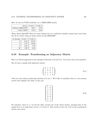
![162 CHAPTER 6. INTRODUCTION TO THRUST PROGRAMMING
Here’s Thrust code to do this:
1 // transgraph problem , using Thrust
2
3 #include <s t d i o . h>
4
5 #include <thrust / d evi ce ve cto r . h>
6 #include <thrust / transform . h>
7 #include <thrust /remove . h>
8 #include <thrust / i t e r a t o r / d i s c a r d i t e r a t o r . h>
9
10 // forms one row of the output matrix
11 s t r u c t makerow {
12 const thrust : : device vector <int >:: i t e r a t o r outmat ;
13 int ∗om;
14 const int nc ; // number of columns
15 makerow( thrust : : device vector <int >:: i t e r a t o r outmat , int nc ) :
16 outmat ( outmat ) , nc ( nc ) { om = thrust : : raw pointer cast (&outmat [ 0 ] ) ; }
17 d e v i c e
18 // the j−th 1 i s in p o s i t i o n i of the ori g matrix
19 bool operator ( ) ( const int i , const int j )
20 { om[2∗ j ] = i / nc ;
21 om[2∗ j +1] = i % nc ;
22 }
23 };
24
25 int main ( int argc , char ∗∗ argv )
26 { int x [ 1 2 ] = {
27 0 ,1 ,1 ,0 ,
28 1 ,0 ,0 ,1 ,
29 1 ,1 ,0 ,0};
30 int nr=3,nc=4, nrc = nr∗nc , i ;
31 thrust : : device vector <int> dx(x , x+nrc ) ;
32 thrust : : device vector <int> ones (x , x+nrc ) ;
33 thrust : : co unt ing it era tor <int> seqb ( 0 ) ;
34 thrust : : co unt ing it era tor <int> seqe = seqb + nrc ;
35 // get 1−D i n d i c e s of the 1 s
36 thrust : : device vector <int >:: i t e r a t o r newend =
37 thrust : : c o p y i f ( seqb , seqe , dx . begin ( ) , ones . begin ( ) ,
38 thrust : : identity <int >());
39 int n1s = newend − ones . begin ( ) ;
40 thrust : : device vector <int> newmat(2∗ n1s ) ;
41 thrust : : device vector <int> out ( n1s ) ;
42 thrust : : co unt ing it era tor <int> seq2b ( 0 ) ;
43 thrust : : transform ( ones . begin ( ) , newend , seq2b ,
44 thrust : : make discard iterator ( ) , makerow(newmat . begin ( ) , nc ) ) ;
45 thrust : : copy (newmat . begin ( ) , newmat . end ( ) ,
46 std : : ostream iterator <int >(std : : cout , ” ” ) ) ;
47 std : : cout << ”n ”;
48 }](https://image.slidesharecdn.com/matloff-programmingonparallelmachines-2013-150626072019-lva1-app6892/85/Matloff-programming-on-parallel_machines-2013-182-320.jpg)
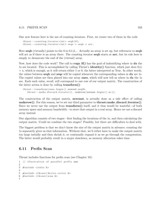
![164 CHAPTER 6. INTRODUCTION TO THRUST PROGRAMMING
8 int main ( int argc , char ∗∗ argv )
9 { int x [ 7 ] = {6 ,12 ,5 ,13 ,3 ,5 ,4};
10 int n=7, i ;
11 thrust : : device vector <int> hx(x , x+n ) ;
12 // in−place scan ; d ef a ul t operation i s +
13 thrust : : i n c l u s i v e s c a n (hx . begin ( ) , hx . end ( ) , hx . begin ( ) ) ;
14 thrust : : copy (hx . begin ( ) , hx . end ( ) ,
15 std : : ostream iterator <int >(std : : cout , ” ” ) ) ;
16 std : : cout << ”n ”;
17 }
6.12 More on Use of Thrust for a CUDA Backend
6.12.1 Synchronicity
Thrust calls are in fact CUDA kernel calls, and thus entail some latency. Other than the transform()-
family functions, the calls are all synchronous.
6.13 Error Messages
A message like
terminate c a l l e d a f t e r throwing an instance of ’ std : : bad alloc ’
what ( ) : std : : bad alloc
may mean that Thrust wasn’t able to allocate your large array on the GPU.
Also, beware of the following. Consider the code
thrust : : device vector <int> seq (n ) ;
thrust : : c o p y i f (hx . begin ( ) , hx . end ( ) , seq , out , ismultk (hx . begin ( ) , i ncr ) ) ;
We forgot the .begin() for seq! If seq had been a non-Thrust array, declared as
int seq [ n ] ;
it would have been fine, but not for a Thrust array.
Unfortunately, the compiler gives us a very long megillah as an error message, a highly uninformative
one. Keep this in mind if you get a 30-line compiler error.
The same thing happens if we forget to state the proper “include” files.](https://image.slidesharecdn.com/matloff-programmingonparallelmachines-2013-150626072019-lva1-app6892/85/Matloff-programming-on-parallel_machines-2013-184-320.jpg)

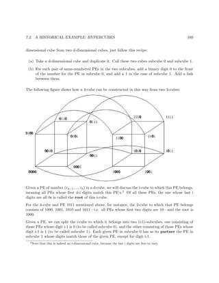

![8.2. REVIEW OF EARLIER EXAMPLE 175
an Infiniband switch to another. Comparing that to the nanosecond time scale of CPU speeds, one
can see that the communications overhead can destroy a program’s performance. And Ethernet is
quite a bit slower than Infiniband.
Latency is quite different from bandwidth, which is the number of bits sent per second. Say the
latency is 1.0 microsecond and the bandwidth is 1 gigabit, i.e. 1000000000 bits per second or 1000
bits per microsecond. Say the message is 2000 bits long. Then the first bit of the message arrives
after 1 microsecond, and the last bit arrives after an additional 2 microseconds. In other words,
the message is does not arrive fully at the destination until 3 microseconds after it is sent.
In the same setting, say bandwidth is 10 gigabits. Now the message would need 1.2 seconds to
arrive fully, in spite of a 10-fold increase in bandwidth. So latency is a major problem even if the
bandwidth is high.
For this reason, the MPI applications that run well on networks tend to be of the “embarrassingly
parallel” type, with very little communication between the processes.
Of course, if your platform is a shared-memory multiprocessor (especially a multicore one, where
communication between cores is particularly fast) and you are running all your MPI processes
on that machine, the problem is less severe. In fact, some implementations of MPI communicate
directly through shared memory in that case, rather than using the TCP/IP or other network
protocol.
8.2 Review of Earlier Example
Though the presentation in this chapter is self-contained, you may wish to look first at the somewhat
simpler example in Section 1.3.3.2, a pipelined prime number finder.
8.3 Example: Dijkstra Algorithm
8.3.1 The Algorithm
The code implements the Dijkstra algorithm for finding the shortest paths in an undirected graph.
Pseudocode for the algorithm is
1 Done = {0}
2 NonDone = {1,2,...,N-1}
3 for J = 1 to N-1 Dist[J] = infinity‘
4 Dist[0] = 0
5 for Step = 1 to N-1
6 find J such that Dist[J] is min among all J in NonDone](https://image.slidesharecdn.com/matloff-programmingonparallelmachines-2013-150626072019-lva1-app6892/85/Matloff-programming-on-parallel_machines-2013-195-320.jpg)
![176 CHAPTER 8. INTRODUCTION TO MPI
7 transfer J from NonDone to Done
8 NewDone = J
9 for K = 1 to N-1
10 if K is in NonDone
11 Dist[K] = min(Dist[K],Dist[NewDone]+G[NewDone,K])
At each iteration, the algorithm finds the closest vertex J to 0 among all those not yet processed,
and then updates the list of minimum distances to each vertex from 0 by considering paths that go
through J. Two obvious potential candidate part of the algorithm for parallelization are the “find
J” and “for K” lines, and the above OpenMP code takes this approach.
8.3.2 The MPI Code
1 // Dijkstra.c
2
3 // MPI example program: Dijkstra shortest-path finder in a
4 // bidirectional graph; finds the shortest path from vertex 0 to all
5 // others
6
7 // command line arguments: nv print dbg
8
9 // where: nv is the size of the graph; print is 1 if graph and min
10 // distances are to be printed out, 0 otherwise; and dbg is 1 or 0, 1
11 // for debug
12
13 // node 0 will both participate in the computation and serve as a
14 // "manager"
15
16 #include <stdio.h>
17 #include <mpi.h>
18
19 #define MYMIN_MSG 0
20 #define OVRLMIN_MSG 1
21 #define COLLECT_MSG 2
22
23 // global variables (but of course not shared across nodes)
24
25 int nv, // number of vertices
26 *notdone, // vertices not checked yet
27 nnodes, // number of MPI nodes in the computation
28 chunk, // number of vertices handled by each node
29 startv,endv, // start, end vertices for this node
30 me, // my node number
31 dbg;
32 unsigned largeint, // max possible unsigned int
33 mymin[2], // mymin[0] is min for my chunk,
34 // mymin[1] is vertex which achieves that min
35 othermin[2], // othermin[0] is min over the other chunks
36 // (used by node 0 only)
37 // othermin[1] is vertex which achieves that min
38 overallmin[2], // overallmin[0] is current min over all nodes,
39 // overallmin[1] is vertex which achieves that min
40 *ohd, // 1-hop distances between vertices; "ohd[i][j]" is](https://image.slidesharecdn.com/matloff-programmingonparallelmachines-2013-150626072019-lva1-app6892/85/Matloff-programming-on-parallel_machines-2013-196-320.jpg)
![8.3. EXAMPLE: DIJKSTRA ALGORITHM 177
41 // ohd[i*nv+j]
42 *mind; // min distances found so far
43
44 double T1,T2; // start and finish times
45
46 void init(int ac, char **av)
47 { int i,j,tmp; unsigned u;
48 nv = atoi(av[1]);
49 dbg = atoi(av[3]);
50 MPI_Init(&ac,&av);
51 MPI_Comm_size(MPI_COMM_WORLD,&nnodes);
52 MPI_Comm_rank(MPI_COMM_WORLD,&me);
53 chunk = nv/nnodes;
54 startv = me * chunk;
55 endv = startv + chunk - 1;
56 u = -1;
57 largeint = u >> 1;
58 ohd = malloc(nv*nv*sizeof(int));
59 mind = malloc(nv*sizeof(int));
60 notdone = malloc(nv*sizeof(int));
61 // random graph
62 // note that this will be generated at all nodes; could generate just
63 // at node 0 and then send to others, but faster this way
64 srand(9999);
65 for (i = 0; i < nv; i++)
66 for (j = i; j < nv; j++) {
67 if (j == i) ohd[i*nv+i] = 0;
68 else {
69 ohd[nv*i+j] = rand() % 20;
70 ohd[nv*j+i] = ohd[nv*i+j];
71 }
72 }
73 for (i = 0; i < nv; i++) {
74 notdone[i] = 1;
75 mind[i] = largeint;
76 }
77 mind[0] = 0;
78 while (dbg) ; // stalling so can attach debugger
79 }
80
81 // finds closest to 0 among notdone, among startv through endv
82 void findmymin()
83 { int i;
84 mymin[0] = largeint;
85 for (i = startv; i <= endv; i++)
86 if (notdone[i] && mind[i] < mymin[0]) {
87 mymin[0] = mind[i];
88 mymin[1] = i;
89 }
90 }
91
92 void findoverallmin()
93 { int i;
94 MPI_Status status; // describes result of MPI_Recv() call
95 // nodes other than 0 report their mins to node 0, which receives
96 // them and updates its value for the global min
97 if (me > 0)
98 MPI_Send(mymin,2,MPI_INT,0,MYMIN_MSG,MPI_COMM_WORLD);](https://image.slidesharecdn.com/matloff-programmingonparallelmachines-2013-150626072019-lva1-app6892/85/Matloff-programming-on-parallel_machines-2013-197-320.jpg)
![178 CHAPTER 8. INTRODUCTION TO MPI
99 else {
100 // check my own first
101 overallmin[0] = mymin[0];
102 overallmin[1] = mymin[1];
103 // check the others
104 for (i = 1; i < nnodes; i++) {
105 MPI_Recv(othermin,2,MPI_INT,i,MYMIN_MSG,MPI_COMM_WORLD,&status);
106 if (othermin[0] < overallmin[0]) {
107 overallmin[0] = othermin[0];
108 overallmin[1] = othermin[1];
109 }
110 }
111 }
112 }
113
114 void updatemymind() // update my mind segment
115 { // for each i in [startv,endv], ask whether a shorter path to i
116 // exists, through mv
117 int i, mv = overallmin[1];
118 unsigned md = overallmin[0];
119 for (i = startv; i <= endv; i++)
120 if (md + ohd[mv*nv+i] < mind[i])
121 mind[i] = md + ohd[mv*nv+i];
122 }
123
124 void disseminateoverallmin()
125 { int i;
126 MPI_Status status;
127 if (me == 0)
128 for (i = 1; i < nnodes; i++)
129 MPI_Send(overallmin,2,MPI_INT,i,OVRLMIN_MSG,MPI_COMM_WORLD);
130 else
131 MPI_Recv(overallmin,2,MPI_INT,0,OVRLMIN_MSG,MPI_COMM_WORLD,&status);
132 }
133
134 void updateallmind() // collects all the mind segments at node 0
135 { int i;
136 MPI_Status status;
137 if (me > 0)
138 MPI_Send(mind+startv,chunk,MPI_INT,0,COLLECT_MSG,MPI_COMM_WORLD);
139 else
140 for (i = 1; i < nnodes; i++)
141 MPI_Recv(mind+i*chunk,chunk,MPI_INT,i,COLLECT_MSG,MPI_COMM_WORLD,
142 &status);
143 }
144
145 void printmind() // partly for debugging (call from GDB)
146 { int i;
147 printf("minimum distances:n");
148 for (i = 1; i < nv; i++)
149 printf("%un",mind[i]);
150 }
151
152 void dowork()
153 { int step, // index for loop of nv steps
154 i;
155 if (me == 0) T1 = MPI_Wtime();
156 for (step = 0; step < nv; step++) {](https://image.slidesharecdn.com/matloff-programmingonparallelmachines-2013-150626072019-lva1-app6892/85/Matloff-programming-on-parallel_machines-2013-198-320.jpg)
![8.3. EXAMPLE: DIJKSTRA ALGORITHM 179
157 findmymin();
158 findoverallmin();
159 disseminateoverallmin();
160 // mark new vertex as done
161 notdone[overallmin[1]] = 0;
162 updatemymind(startv,endv);
163 }
164 updateallmind();
165 T2 = MPI_Wtime();
166 }
167
168 int main(int ac, char **av)
169 { int i,j,print;
170 init(ac,av);
171 dowork();
172 print = atoi(av[2]);
173 if (print && me == 0) {
174 printf("graph weights:n");
175 for (i = 0; i < nv; i++) {
176 for (j = 0; j < nv; j++)
177 printf("%u ",ohd[nv*i+j]);
178 printf("n");
179 }
180 printmind();
181 }
182 if (me == 0) printf("time at node 0: %fn",(float)(T2-T1));
183 MPI_Finalize();
184 }
185
The various MPI functions will be explained in the next section.
8.3.3 Introduction to MPI APIs
8.3.3.1 MPI Init() and MPI Finalize()
These are required for starting and ending execution of an MPI program. Their actions may be
implementation-dependent. For instance, if our platform is an Ethernet-based cluster , MPI Init()
will probably set up the TCP/IP sockets via which the various nodes communicate with each
other. On an Infiniband-based cluster, connections in the special Infiniband network protocol will
be established. On a shared-memory multiprocessor, an implementation of MPI that is tailored to
that platform would take very different actions.
8.3.3.2 MPI Comm size() and MPI Comm rank()
In our function init() above, note the calls](https://image.slidesharecdn.com/matloff-programmingonparallelmachines-2013-150626072019-lva1-app6892/85/Matloff-programming-on-parallel_machines-2013-199-320.jpg)
![182 CHAPTER 8. INTRODUCTION TO MPI
8.4 Example: Removing 0s from an Array
1 #include <mpi . h>
2 #include <s t d l i b . h>
3
4 #define MAX N 100000
5 #define MAX NPROCS 100
6 #define DATA MSG 0
7 #define NEWDATAMSG 1
8
9 int nnodes , // number of MPI processes
10 n , // s i z e of o r i g i n a l array
11 me, // my MPI ID
12 has0s [MAX N] , // o r i g i n a l data
13 no0s [MAX N] , // 0−f r e e data
14 nno0s ; // number of non−0 elements
15
16 int debug ;
17
18 i n i t ( int argc , char ∗∗ argv )
19 {
20 int i ;
21 MPI Init(&argc ,&argv ) ;
22 MPI Comm size (MPI COMM WORLD,&nnodes ) ;
23 MPI Comm rank(MPI COMM WORLD,&me ) ;
24 n = a t oi ( argv [ 1 ] ) ;
25 i f (me == 0) {
26 f o r ( i = 0; i < n ; i++)
27 has0s [ i ] = rand () % 4;
28 } e l s e {
29 debug = at o i ( argv [ 2 ] ) ;
30 while ( debug ) ;
31 }
32 }
33
34 void managernode ()
35 {
36 MPI Status status ;
37 int i ;
38 int lenchunk ;
39 lenchunk = n / ( nnodes −1); // assumed divides evenly
40 f o r ( i = 1; i < nnodes ; i++) {
41 MPI Send ( has0s+(i −1)∗lenchunk , lenchunk ,
42 MPI INT , i ,DATA MSG,MPI COMM WORLD) ;
43 }
44 int k = 0;
45 f o r ( i = 1; i < nnodes ; i++) {
46 MPI Recv( no0s+k ,MAX N,
47 MPI INT , i ,NEWDATAMSG,MPI COMM WORLD,& status ) ;](https://image.slidesharecdn.com/matloff-programmingonparallelmachines-2013-150626072019-lva1-app6892/85/Matloff-programming-on-parallel_machines-2013-202-320.jpg)
![8.5. DEBUGGING MPI CODE 183
48 MPI Get count(&status , MPI INT,& lenchunk ) ;
49 k += lenchunk ;
50 }
51 nno0s = k ;
52 }
53
54 void remov0s ( int ∗oldx , int n , int ∗newx , int ∗nnewx)
55 { int i , count = 0;
56 f o r ( i = 0; i < n ; i++)
57 i f ( oldx [ i ] != 0) newx [ count++] = oldx [ i ] ;
58 ∗nnewx = count ;
59 }
60
61 void workernode ()
62 {
63 int lenchunk ;
64 MPI Status status ;
65 MPI Recv( has0s ,MAX N,
66 MPI INT , 0 ,DATA MSG,MPI COMM WORLD,& status ) ;
67 MPI Get count(&status , MPI INT,& lenchunk ) ;
68 remov0s ( has0s , lenchunk , no0s ,&nno0s ) ;
69 MPI Send ( no0s , nno0s ,
70 MPI INT , 0 ,NEWDATAMSG,MPI COMM WORLD) ;
71 }
72
73 int main ( int argc , char ∗∗ argv )
74 {
75 int i ;
76 i n i t ( argc , argv ) ;
77 i f (me == 0 && n < 25) {
78 f o r ( i = 0; i < n ; i++) p r i n t f (”%d ” , has0s [ i ] ) ;
79 p r i n t f (”n ” ) ;
80 }
81 i f (me == 0) managernode ( ) ;
82 e l s e workernode ( ) ;
83 i f (me == 0 && n < 25) {
84 f o r ( i = 0; i < n ; i++) p r i n t f (”%d ” , no0s [ i ] ) ;
85 p r i n t f (”n ” ) ;
86 }
87 MPI Finalize ( ) ;
88 }
8.5 Debugging MPI Code
If you are using GDB—either directly, or via an IDE such as Eclipse or Netbeans—the trick with
MPI is to attach GDB to your running MPI processes.
Set up code like that we’ve seen in our examples here:](https://image.slidesharecdn.com/matloff-programmingonparallelmachines-2013-150626072019-lva1-app6892/85/Matloff-programming-on-parallel_machines-2013-203-320.jpg)
![8.6. COLLECTIVE COMMUNICATIONS 185
22 *notdone, // vertices not checked yet
23 nnodes, // number of MPI nodes in the computation
24 chunk, // number of vertices handled by each node
25 startv,endv, // start, end vertices for this node
26 me, // my node number
27 dbg;
28 unsigned largeint, // max possible unsigned int
29 mymin[2], // mymin[0] is min for my chunk,
30 // mymin[1] is vertex which achieves that min
31 overallmin[2], // overallmin[0] is current min over all nodes,
32 // overallmin[1] is vertex which achieves that min
33 *ohd, // 1-hop distances between vertices; "ohd[i][j]" is
34 // ohd[i*nv+j]
35 *mind; // min distances found so far
36
37 double T1,T2; // start and finish times
38
39 void init(int ac, char **av)
40 { int i,j,tmp; unsigned u;
41 nv = atoi(av[1]);
42 dbg = atoi(av[3]);
43 MPI_Init(&ac,&av);
44 MPI_Comm_size(MPI_COMM_WORLD,&nnodes);
45 MPI_Comm_rank(MPI_COMM_WORLD,&me);
46 chunk = nv/nnodes;
47 startv = me * chunk;
48 endv = startv + chunk - 1;
49 u = -1;
50 largeint = u >> 1;
51 ohd = malloc(nv*nv*sizeof(int));
52 mind = malloc(nv*sizeof(int));
53 notdone = malloc(nv*sizeof(int));
54 // random graph
55 // note that this will be generated at all nodes; could generate just
56 // at node 0 and then send to others, but faster this way
57 srand(9999);
58 for (i = 0; i < nv; i++)
59 for (j = i; j < nv; j++) {
60 if (j == i) ohd[i*nv+i] = 0;
61 else {
62 ohd[nv*i+j] = rand() % 20;
63 ohd[nv*j+i] = ohd[nv*i+j];
64 }
65 }
66 for (i = 0; i < nv; i++) {
67 notdone[i] = 1;
68 mind[i] = largeint;
69 }
70 mind[0] = 0;
71 while (dbg) ; // stalling so can attach debugger
72 }
73
74 // finds closest to 0 among notdone, among startv through endv
75 void findmymin()
76 { int i;
77 mymin[0] = largeint;
78 for (i = startv; i <= endv; i++)
79 if (notdone[i] && mind[i] < mymin[0]) {](https://image.slidesharecdn.com/matloff-programmingonparallelmachines-2013-150626072019-lva1-app6892/85/Matloff-programming-on-parallel_machines-2013-205-320.jpg)
![186 CHAPTER 8. INTRODUCTION TO MPI
80 mymin[0] = mind[i];
81 mymin[1] = i;
82 }
83 }
84
85 void updatemymind() // update my mind segment
86 { // for each i in [startv,endv], ask whether a shorter path to i
87 // exists, through mv
88 int i, mv = overallmin[1];
89 unsigned md = overallmin[0];
90 for (i = startv; i <= endv; i++)
91 if (md + ohd[mv*nv+i] < mind[i])
92 mind[i] = md + ohd[mv*nv+i];
93 }
94
95 void printmind() // partly for debugging (call from GDB)
96 { int i;
97 printf("minimum distances:n");
98 for (i = 1; i < nv; i++)
99 printf("%un",mind[i]);
100 }
101
102 void dowork()
103 { int step, // index for loop of nv steps
104 i;
105 if (me == 0) T1 = MPI_Wtime();
106 for (step = 0; step < nv; step++) {
107 findmymin();
108 MPI_Reduce(mymin,overallmin,1,MPI_2INT,MPI_MINLOC,0,MPI_COMM_WORLD);
109 MPI_Bcast(overallmin,1,MPI_2INT,0,MPI_COMM_WORLD);
110 // mark new vertex as done
111 notdone[overallmin[1]] = 0;
112 updatemymind(startv,endv);
113 }
114 // now need to collect all the mind values from other nodes to node 0
115 MPI_Gather(mind+startv,chunk,MPI_INT,mind,chunk,MPI_INT,0,MPI_COMM_WORLD);
116 T2 = MPI_Wtime();
117 }
118
119 int main(int ac, char **av)
120 { int i,j,print;
121 init(ac,av);
122 dowork();
123 print = atoi(av[2]);
124 if (print && me == 0) {
125 printf("graph weights:n");
126 for (i = 0; i < nv; i++) {
127 for (j = 0; j < nv; j++)
128 printf("%u ",ohd[nv*i+j]);
129 printf("n");
130 }
131 printmind();
132 }
133 if (me == 0) printf("time at node 0: %fn",(float)(T2-T1));
134 MPI_Finalize();
135 }](https://image.slidesharecdn.com/matloff-programmingonparallelmachines-2013-150626072019-lva1-app6892/85/Matloff-programming-on-parallel_machines-2013-206-320.jpg)
![190 CHAPTER 8. INTRODUCTION TO MPI
MPI Scatter (oh , lenchunk , MPI INT , ohchunk , lenchunk , MPI INT , 0 ,
MPI COMM WORLD) ;
means
Node 0 will break up the array oh of type MPI INT into chunks of length lenchunk,
sending the ith chunk to Node i, where lenchunk items will be deposited at ohchunk.
8.6.6 Example: Count the Number of Edges in a Directed Graph
Below is MPI code to count the number of edges in a directed graph. (“Directed” means that a
link from i to j does not necessarily imply one from j to i.)
In the context here, me is the node’s rank; nv is the number of vertices; oh is the one-hop distance
matrix; and nnodes is the number of MPI processes. At the beginning only the process of rank 0
has a copy of oh, but it sends that matrix out in chunks to the other nodes, each of which stores
its chunk in an array ohchunk.
1 lenchunk = nv / nnodes ;
2 MPI Scatter (oh , lenchunk , MPI INT , ohchunk , lenchunk , MPI INT , 0 ,
3 MPI COMM WORLD) ;
4 mycount = 0;
5 f o r ( i = 0; i < nv∗nv/nnodes )
6 i f ( ohchunk [ i ] != 0) mycount++;
7 MPI Reduce(&mycount,&numedge , 1 , MPI INT ,MPI SUM, 0 ,MPI COMM WORLD) ;
8 i f (me == 0) p r i n t f (” there are %d edges n” ,numedge ) ;
8.6.7 Example: Cumulative Sums
Here we find cumulative sums. For instance, if the original array is (3,1,2,0,3,0,1,2), then it is
changed to (3,4,6,6,9,9,10,12). (This topic is pursued in depth in Chapter 10.)
1 // f i n d s cumulative sums in the array x
2
3 #include <mpi . h>
4 #include <s t d l i b . h>
5
6 #define MAX N 10000000
7 #define MAX NODES 10
8
9 int nnodes , // number of MPI processes
10 n , // s i z e of x
11 me, // MPI rank of t h i s node
12 // f u l l data f o r node 0 , part f o r the r e s t](https://image.slidesharecdn.com/matloff-programmingonparallelmachines-2013-150626072019-lva1-app6892/85/Matloff-programming-on-parallel_machines-2013-210-320.jpg)
![8.6. COLLECTIVE COMMUNICATIONS 191
13 x [MAX N] ,
14 csums [MAX N] , // cumulative sums f o r t h i s node
15 maxvals [MAX NODES] ; // the max values at the various nodes
16
17 int debug ;
18
19 i n i t ( int argc , char ∗∗ argv )
20 {
21 int i ;
22 MPI Init(&argc ,&argv ) ;
23 MPI Comm size (MPI COMM WORLD,&nnodes ) ;
24 MPI Comm rank(MPI COMM WORLD,&me ) ;
25 n = a t oi ( argv [ 1 ] ) ;
26 // t e s t data
27 i f (me == 0) {
28 f o r ( i = 0; i < n ; i++)
29 x [ i ] = rand () % 32;
30 }
31 debug = at o i ( argv [ 2 ] ) ;
32 while ( debug ) ;
33 }
34
35 void cumulsums ()
36 {
37 MPI Status status ;
38 int i , lenchunk , sum , node ;
39 lenchunk = n / nnodes ; // assumed to divide evenly
40 // note that node 0 w i l l p a r t i c i p a t e in the computation too
41 MPI Scatter (x , lenchunk , MPI INT , x , lenchunk , MPI INT ,
42 0 ,MPI COMM WORLD) ;
43 sum = 0;
44 f o r ( i = 0; i < lenchunk ; i++) {
45 csums [ i ] = sum + x [ i ] ;
46 sum += x [ i ] ;
47 }
48 MPI Gather(&csums [ lenchunk −1] ,1 ,MPI INT ,
49 maxvals , 1 , MPI INT , 0 ,MPI COMM WORLD) ;
50 MPI Bcast ( maxvals , nnodes , MPI INT , 0 ,MPI COMM WORLD) ;
51 i f (me > 0) {
52 sum = 0;
53 f o r ( node = 0; node < me; node++) {
54 sum += maxvals [ node ] ;
55 }
56 f o r ( i = 0; i < lenchunk ; i++)
57 csums [ i ] += sum ;
58 }
59 MPI Gather ( csums , lenchunk , MPI INT , csums , lenchunk , MPI INT ,
60 0 ,MPI COMM WORLD) ;
61 }
62](https://image.slidesharecdn.com/matloff-programmingonparallelmachines-2013-150626072019-lva1-app6892/85/Matloff-programming-on-parallel_machines-2013-211-320.jpg)
![192 CHAPTER 8. INTRODUCTION TO MPI
63 int main ( int argc , char ∗∗ argv )
64 {
65 int i ;
66 i n i t ( argc , argv ) ;
67 i f (me == 0 && n < 25) {
68 f o r ( i = 0; i < n ; i++) p r i n t f (”%d ” ,x [ i ] ) ;
69 p r i n t f (”n ” ) ;
70 }
71 cumulsums ( ) ;
72 i f (me == 0 && n < 25) {
73 f o r ( i = 0; i < n ; i++) p r i n t f (”%d ” , csums [ i ] ) ;
74 p r i n t f (”n ” ) ;
75 }
76 MPI Finalize ( ) ;
77 }
8.6.8 Example: an MPI Solution to the Mutual Outlinks Problem
Consider the example of Section 2.4.3. We have a network graph of some kind, such as Web
links. For any two vertices, say any two Web sites, we might be interested in mutual outlinks, i.e.
outbound links that are common to two Web sites.
The MPI code below finds the mean number of mutual outlinks, among all pairs of vertices in a
graph.
1 // MPI s o l u t i o n to the mutual o u t l i n k s problem
2
3 // adjacency matrix m i s global at each node , broadcast from node 0
4
5 // assumes m i s nxn , and number of nodes i s < n
6
7 // f o r each node i , check a l l p o s s i b l e pairing nodes j > i ; the various
8 // nodes work on values of i in a Round Robin fashion , with node k
9 // handling a l l i f o r which i mod nnodes = k
10
11 #include <mpi . h>
12 #include <s t d l i b . h>
13
14 #define MAXLENGTH 10000000
15
16 int nnodes , // number of MPI processes
17 n , // s i z e of x
18 me, // MPI rank of t h i s node
19 m[MAXLENGTH] , // adjacency matrix
20 grandtot ; // grand t o t a l of a l l counts of mutuality
21
22 // get adjacency matrix , in t h i s case j u s t by simulation
23 void getm ()](https://image.slidesharecdn.com/matloff-programmingonparallelmachines-2013-150626072019-lva1-app6892/85/Matloff-programming-on-parallel_machines-2013-212-320.jpg)
![8.6. COLLECTIVE COMMUNICATIONS 193
24 { int i ;
25 f o r ( i = 0; i < n∗n ; i++)
26 m[ i ] = rand () % 2;
27 }
28
29 i n i t ( int argc , char ∗∗ argv )
30 {
31 int i ;
32 MPI Init(&argc ,&argv ) ;
33 MPI Comm size (MPI COMM WORLD,&nnodes ) ;
34 MPI Comm rank(MPI COMM WORLD,&me ) ;
35 n = a t oi ( argv [ 1 ] ) ;
36 i f (me == 0) {
37 getm ( ) ; // get the data (app−s p e c i f i c )
38 }
39 }
40
41 void mutlinks ()
42 {
43 int i , j , k , tot ;
44 MPI Bcast (m, n∗n , MPI INT , 0 ,MPI COMM WORLD) ;
45 tot = 0;
46 f o r ( i = me; i < n−1; i += nnodes ) {
47 f o r ( j = i +1; j < n ; j++) {
48 f o r (k = 0; k < n ; k++)
49 tot += m[ twod2oned (n , i , k ) ] ∗ m[ twod2oned (n , j , k ) ] ;
50 }
51 }
52 MPI Reduce(&tot ,& grandtot , 1 , MPI INT ,MPI SUM, 0 ,MPI COMM WORLD) ;
53 }
54
55 // convert 2−D subscript to 1−D
56 int twod2oned (n , i , j )
57 { return n ∗ i + j ; }
58
59 int main ( int argc , char ∗∗ argv )
60 { int i , j ;
61 i n i t ( argc , argv ) ;
62 i f (me == 0 && n < 5) { // check t e s t input
63 f o r ( i = 0; i < n ; i++) {
64 f o r ( j = 0; j < n ; j++) p r i n t f (”%d ” ,m[ twod2oned (n , i , j ) ] ) ;
65 p r i n t f (”n ” ) ;
66 }
67 }
68 mutlinks ( ) ;
69 i f (me == 0) p r i n t f (”% f n ” ,(( f l o a t ) grandtot )/( n∗(n −1)/2));
70 MPI Finalize ( ) ;
71 }](https://image.slidesharecdn.com/matloff-programmingonparallelmachines-2013-150626072019-lva1-app6892/85/Matloff-programming-on-parallel_machines-2013-213-320.jpg)
![194 CHAPTER 8. INTRODUCTION TO MPI
8.6.9 The MPI Barrier()
This implements a barrier for a given communicator. The name of the communicator is the sole
argument for the function.
Explicit barriers are less common in message-passing programs than in the shared-memory world.
8.6.10 Creating Communicators
Again, a communicator is a subset (either proper or improper) of all of our nodes. MPI includes a
number of functions for use in creating communicators. Some set up a virtual “topology” among
the nodes.
For instance, many physics problems consist of solving differential equations in two- or three-
dimensional space, via approximation on a grid of points. In two dimensions, groups may consists
of rows in the grid.
Here’s how we might divide an MPI run into two groups (assumes an even number of MPI processes
to begin with):
MPI_Comm_size(MPI_COMM_WORLD,&nnodes);
MPI_Comm_rank(MPI_COMM_WORLD,&me);
...
// declare variables to bind to groups
MPI_Group worldgroup, subgroup;
// declare variable to bind to a communicator
MPI_Comm subcomm;
...
int i,startrank,nn2 = nnodes/2;
int *subranks = malloc(nn2*sizeof(int));
if (me < nn2) start = 0;
else start = nn2;
for (i = 0; i < nn2; i++)
subranks[i] = i + start;
// bind the world to a group variable
MPI_Comm_group(MPI_COMM_WORLD, &worldgroup);
// take worldgroup the nn2 ranks in "subranks" and form group
// "subgroup" from them
MPI_Group_incl(worldgroup, nn2, subranks, subgroup);
// create a communicator for that new group
MPI_Comm_create(MPI_COMM_WORLD, subgroup, subcomm);
// get my rank in this new group
MPI_Group_rank (subgroup, &subme);
You would then use subcomm instead of MPI COMM WORLD whenever you wish to, say, broad-
cast, only to that group.](https://image.slidesharecdn.com/matloff-programmingonparallelmachines-2013-150626072019-lva1-app6892/85/Matloff-programming-on-parallel_machines-2013-214-320.jpg)
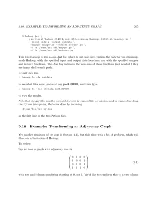
![9.10. EXAMPLE: TRANSFORMING AN ADJACENCY GRAPH 207
5 # row (3 ,8) in the f i n a l output
6
7 import sys
8
9 f o r l i n e in sys . stdin :
10 tks = l i n e . s p l i t () # get tokens
11 srcnode = tks [ 0 ]
12 l i n k s = tks [ 1 : ]
13 f o r dstnode in range ( len ( l i n k s ) ) :
14 i f l i n k s [ dstnode ] == ’ 1 ’ :
15 toprint = ’%s t%s ’ % ( srcnode , dstnode )
16 print toprint
And the reducer code:
1 #!/ usr / bin /env python
2
3 import sys
4
5 f o r l i n e in sys . stdin :
6 l i n e = l i n e . s t r i p ()
7 print l i n e # could remove the t
Note that the row number, needed for other reasons, is also serving as our Hadoop key variable.
Recall that in the word count and yearly temperature examples above, the reducer did the main
work, with the mappers playing only a supporting role. In this case here, it’s the opposite, with the
reducers doing little more than printing what they’re given. However, keep in mind that Hadoop
itself did a lot of the work, with its shuffle phase, which produced the sorting that we required in
the output.
Here’s the same code in R:
mapper:
1 #!/ usr / bin /env Rscript
2
3 # map/ reduce pair inputs a graph adjacency matrix and outputs a l i s t of
4 # l i n k s ; i f say row 3 , column 8 of the input i s 1 , then there w i l l be a
5 # row (3 ,8) in the f i n a l output
6
7 con <− f i l e (” stdin ” , open = ” r ”)
8 mapin <− readLines ( con ) # better not to read a l l at once , but keep simple
9 f o r ( l i n e in mapin ) {
10 tks <− s t r s p l i t ( line , s p l i t =” ”)
11 tks <− tks [ [ 1 ] ]
12 srcnode <− tks [ 1 ]
13 l i n k s <− tks [ −1]
14 f o r ( dstnode in 1: length ( l i n k s )) {
15 i f ( l i n k s [ dstnode ] == ’1 ’)](https://image.slidesharecdn.com/matloff-programmingonparallelmachines-2013-150626072019-lva1-app6892/85/Matloff-programming-on-parallel_machines-2013-227-320.jpg)
![208 CHAPTER 9. CLOUD COMPUTING
16 cat ( srcnode ,” t ” , dstnode ,” n” , sep =””)
17 }
18 }
reducer:
1 #!/ usr / bin /env Rscript
2
3 con <− f i l e (” stdin ” , open = ” r ”)
4 mapin <− readLines ( con )
5 f o r ( l i n e in mapin ) {
6 l i n e <− s t r s p l i t ( line , s p l i t =”t ”) # remove t
7 l i n e <− l i n e [ [ 1 ] ]
8 cat ( line ,” n”)
9 }
9.11 Example: Identifying Outliers
In any large data set, there are various errors, say 3-year-olds who are listed as 7 feet tall. One
way to try to track these down is to comb the data for outliers, which are data points (rows in the
data set) that are far from the others. These may not be erroneous, but they are “suspicious,” and
we want to flag them for closer inspection.
In this simple version, we will define an outlier point to be one for which at least one of its variables
is in the upper p proportion in its group. Say for example p is 0.02, and our groups are male adults
and female adults, with our data variables being height and weight. Then if the height for some
man were in the upper 2% of all men in the data set, we’d flag him as an outlier; we’d do the same
for weight. Note that he’d be selected if either his height or his weight were in the top 2% for that
variable among men in the data set. Of course, we could also look at the bottom 2%, or those
whose Euclidean distance as vectors are in the most distant 2% from the centroid of the data in a
group, etc.
We’ll define groups in terms of combinations of variables. These might be, say, Asian male lawyers,
female Kentucky natives registered as Democrats, etc.
mapper:
1 #!/ usr / bin /env Rscript
2
3 # map/ reduce pair inputs a data matrix , forms groups according to
4 # combinations of s p e c i f i e d i n t e g e r variables , and then outputs the
5 # i n d i c e s of o u t l i e r s in each group
6
7 # any observation that has at l e a s t one v a r i a b l e in the top p% of i t s
8 # group i s considered an o u t l i e r](https://image.slidesharecdn.com/matloff-programmingonparallelmachines-2013-150626072019-lva1-app6892/85/Matloff-programming-on-parallel_machines-2013-228-320.jpg)
![9.11. EXAMPLE: IDENTIFYING OUTLIERS 209
9
10 # the f i r s t column of the input matrix i s the observation number ,
11 # s t a r t i n g at 0
12
13 # the group number f o r an observation i s the l i n e a r index in
14 # l e x i c o g r a p h i c a l terms
15
16 # in Hadoop command line , use −mapper ”olmap .R ’0.4 2 3 6 16 ’” to
17 # s p e c i f y parameters :
18
19 # p ( given as a decimal number , e . g . 0 . 0 2 ) ; d , the number
20 # of data v a r i a b l e s ; g , the number of grouping v a r i a b l e s ; and f i n a l l y g
21 # numbers which are the upper bounds f o r the l a s t g−1 group v a r i a b l e s
22 # ( the lower bounds are always assumed to be 0)
23
24 i n i t <− function () {
25 ca <− commandArgs( trailingOnly=T)
26 pars <− ca [ 1 ]
27 pars <− s t r s p l i t ( pars , s p l i t =” ” ) [ [ 1 ] ]
28 pars <− pars [ −1]
29 ndv <<− as . i n t e g e r ( pars [ 1 ] )
30 ngv <<− as . i n t e g e r ( pars [ 2 ] )
31 # a few p o s i t i o n variables , used in findgrp () below
32 grpstart <<− 2
33 grpend <<− grpstart + ngv − 1
34 datastart <<− 2+ngv
35 dataend <<− 1 + ngv + ndv
36 # get upper bounds , and t h e i r reverse −cumulative products
37 ubds <<− as . i n t e g e r ( pars [3:(1+ ngv ) ] )
38 ubdsprod <<− vector ( length=ngv−1)
39 f o r ( i in 1 : ( ngv −1))
40 ubdsprod [ i ] <<− prod ( ubds [ i : ( ngv −1)])
41 }
42
43 # converts vector of group v a r i a b l e s to group number
44 findgrp <− function ( grpvars ) {
45 sum <− 0
46 f o r ( i in 1 : ( ngv −1)) {
47 m <− grpvars [ i ]
48 sum <− sum + m ∗ ubdsprod [ i ]
49 }
50 return (sum+grpvars [ ngv ] )
51 }
52
53 # t e s t
54 i n i t ()
55 con <− f i l e (” stdin ” , open = ” r ”)
56 mapin <− readLines ( con ) # better not to read a l l at once
57 f o r ( l i n e in mapin ) {
58 tks <− s t r s p l i t ( line , s p l i t =” ”)](https://image.slidesharecdn.com/matloff-programmingonparallelmachines-2013-150626072019-lva1-app6892/85/Matloff-programming-on-parallel_machines-2013-229-320.jpg)
![210 CHAPTER 9. CLOUD COMPUTING
59 tks <− tks [ [ 1 ] ]
60 rownum <− tks [ 1 ]
61 grpvars <− tks [ grpstart : grpend ]
62 grpvars <− as . i n t e g e r ( grpvars )
63 grpnum <− findgrp ( grpvars )
64 cat (grpnum ,” t ” ,rownum ,” ” , tks [ datastart : dataend ] ,” n”)
65 }
reducer:
1 #!/ usr / bin /env Rscript
2
3 # see comments in olmap .R
4
5 # in Hadoop command line , use −reducer ” olred .R ’0.4 2 3 6 16 ’” or
6 # s i m i l a r
7
8 # R’ s quantile () too complicated
9 quantl <− function (x , q) {
10 return ( sort (x ) [ c e i l i n g ( length (x)∗q ) ] )
11 }
12
13 i n i t <− function () {
14 ca <− commandArgs( trailingOnly=T)
15 pars <− ca [ 1 ]
16 pars <− s t r s p l i t ( pars , s p l i t =” ” ) [ [ 1 ] ]
17 # pars <− c (”0.4” ,”2” ,”3” ,”6” ,”16”) # f o r l i t t l e t e s t
18 # pars <− c (”0.1” ,”2” ,”2” ,”3”) # f o r big t e s t
19 p <<− as . double ( pars [ 1 ] )
20 ndv <<− as . i n t e g e r ( pars [ 2 ] )
21 }
22
23 e m i t o u t l i e r s <− function ( datamat ) {
24 # find the upper p quantile f o r each v a r i a b l e ( skip row number)
25 toohigh <− apply ( datamat [ , −(1:2) , drop=F] , 2 , quantl ,1−p)
26 f o r ( i in 1: nrow ( datamat )) {
27 i f ( any ( datamat [ i , −(1:2)] >= toohigh ))
28 cat ( datamat [ i , ] , ” n”)
29 }
30 }
31
32 # t e s t
33 i n i t ()
34 con <− f i l e (” stdin ” , open = ” r ”)
35 mapin <− readLines ( con )
36 oldgrpnum <− −1
37 nmapin <− length ( mapin )
38 f o r ( i in 1: nmapin ) {
39 l i n e <− mapin [ i ]
40 tks <− s t r s p l i t ( line , s p l i t =”t ” ) [ [ 1 ] ]](https://image.slidesharecdn.com/matloff-programmingonparallelmachines-2013-150626072019-lva1-app6892/85/Matloff-programming-on-parallel_machines-2013-230-320.jpg)
![9.12. DEBUGGING HADOOP STREAMING PROGRAMS 211
41 grpnum <− as . i n t e g e r ( tks [ 1 ] )
42 tmp <− s t r s p l i t ( tks [ 2 ] , s p l i t =” ” ) [ [ 1 ] ]
43 tmp <− tmp [ tmp != ””] # d e l e t e empty element
44 row <− as . numeric (tmp)
45 i f ( oldgrpnum == −1) {
46 datamat <− matrix ( c (grpnum , row ) , nrow=1)
47 oldgrpnum <− grpnum
48 } e l s e i f (grpnum == oldgrpnum ) {
49 datamat <− rbind ( datamat , c (grpnum , row ))
50 i f ( i == nmapin ) e m i t o u t l i e r s ( datamat )
51 } e l s e { # new group
52 e m i t o u t l i e r s ( datamat )
53 datamat <− matrix ( c (grpnum , row ) , nrow=1)
54 oldgrpnum <− grpnum
55 }
56 }
9.12 Debugging Hadoop Streaming Programs
One advantage of the streaming approach is that mapper and reducer programs can be debugged
via normal tools, since those programs can be run on their own, without Hadoop, simply by using
the Unix/Linux pipe capability.
This all depends on the fact that Hadoop essentially does the following Unix shell computation:
cat i n p u t f i l e | mapperprog | sort −n | reducerprog
(Omit the -n if the key is a string.)
The mapper alone works like
cat i n p u t f i l e | mapperprog
You thus can use whatever debugging tool you favor, to debug the mapper and reducer code
separately.
Note, though, that the above pipe is not quite the same as Hadoop. the pipe doesn’t break up
the data, and there may be subtle problems arising as a result. But overall, the above approach
provides a quick and easy first attempt at debugging.
The userlogs subdirectory of your Hadoop logs directory contains files that may be helpful, such
as stderr.](https://image.slidesharecdn.com/matloff-programmingonparallelmachines-2013-150626072019-lva1-app6892/85/Matloff-programming-on-parallel_machines-2013-231-320.jpg)
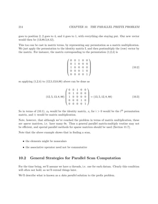
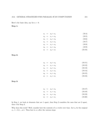
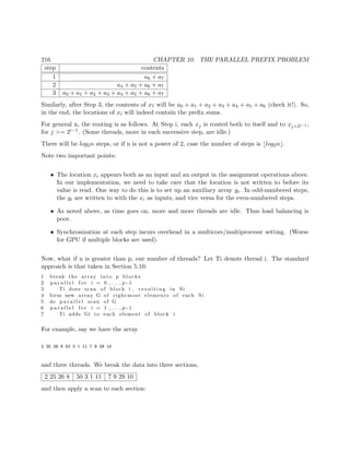
![10.3. IMPLEMENTATIONS 217
2 27 53 61 50 53 54 65 7 16 45 55
But we still don’t have the scan of the array overall. That 50, for instance, should be 61+50 =
111 and the 53 should be 61+53 = 114. In other words, 61 must be added to that second section,
(50,53,54,65), and 61+65 = 126 must be added to the third section, (7,16,45,55). This then is the
last step, yielding
2 27 53 61 111 114 115 126 133 142 171 181
Another possible approach would be make n “fake” threads FTj. Each Ti plays the role of n/p
of the FTj. The FTj then do the parallel scan as at the beginning of this section. Key point:
Whenever a Ti becomes idle, it is assigned to help other Tk.
10.3 Implementations
The MPI standard actually includes built-in parallel prefix functions, MPI Scan(). A number of
choices are offered for ⊗, such as maximum, minimum, sum, product etc.
The Thrust library for CUDA or OpenMP includes functions thrust::inclusive scan() and thrust::exclusive sca
The CUDPP (CUDA Data Parallel Primitives Library) package contains CUDA functions for
sorting and other operations, many of which are based on parallel scan. See http://gpgpu.
org/developer/cudpp for the library code, and a detailed analysis of optimizing parallel pre-
fix in a GPU context in the book GPU Gems 3, available either in bookstores or free online at
http://developer.nvidia.com/object/gpu_gems_home.html.
10.4 Example: Parallel Prefix, Run-Length Decoding in OpenMP
Here an OpenMP implementation of the approach described at the end of Section 10.2, for addition:
1 #include <omp. h>
2
3 // c a l c u l a t e s p r e f i x sums s e q u e n t i a l l y on u , in−place , where u i s an
4 // m−element array
5 void seqprfsum ( int ∗u , int m)
6 { int i , s=u [ 0 ] ;
7 f o r ( i = 1; i < m; i++) {
8 u [ i ] += s ;
9 s = u [ i ] ;
10 }
11 }
12
13 // OMP example , c a l c u l a t i n g p r e f i x sums in p a r a l l e l on the n−element](https://image.slidesharecdn.com/matloff-programmingonparallelmachines-2013-150626072019-lva1-app6892/85/Matloff-programming-on-parallel_machines-2013-237-320.jpg)
![218 CHAPTER 10. THE PARALLEL PREFIX PROBLEM
14 // array x , in−place ; f o r simplicity , assume that n i s d i v i s i b l e by the
15 // number of threads ; z i s f o r intermediate storage , an array with length
16 // equal to the number of threads ; x and z point to global arrays
17 void parprfsum ( int ∗x , int n , int ∗z )
18 {
19 #pragma omp p a r a l l e l
20 { int i , j ,me = omp get thread num ( ) ,
21 nth = omp get num threads ( ) ,
22 chunksize = n / nth ,
23 s t a r t = me ∗ chunksize ;
24 seqprfsum(&x [ s t a r t ] , chunksize ) ;
25 #pragma omp b a r r i e r
26 #pragma omp s i n g l e
27 {
28 f o r ( i = 0; i < nth −1; i++)
29 z [ i ] = x [ ( i +1)∗ chunksize − 1 ] ;
30 seqprfsum ( z , nth −1);
31 }
32 i f (me > 0) {
33 f o r ( j = s t a r t ; j < s t a r t + chunksize ; j++) {
34 x [ j ] += z [me − 1 ] ;
35 }
36 }
37 }
38 }
Here is an example of use: A method for compressing data is to store only repeat counts in
runs, where the latter means a set of consecutive, identical values. For instance, the sequence
2,2,2,0,0,5,0,0 would be compressed to 3,2,2,0,1,5,2,0, meaning that the data consist of first three
2s, then two 0s, then one 5, and finally two 0s. Note that the compressed version consists of
alternating run counts and run values, respectively 2 and 0 at the end of the above example.
To solve this in OpenMP, we’ll first call the above functions to decide where to place the runs in
our overall output.
1 void uncomprle ( int ∗x , int nx , int ∗tmp , int ∗y , int ∗ny)
2 {
3 int i , nx2 = nx /2;
4 int z [MAXTHREADS] ;
5 f o r ( i = 0; i < nx2 ; i++) tmp [ i +1] = x [2∗ i ] ;
6 parprfsum (tmp+1,nx2+1,z ) ;
7 tmp [ 0 ] = 0;
8 #pragma omp p a r a l l e l
9 { int j , k ;
10 int me=omp get thread num ( ) ;
11 #pragma omp f o r
12 f o r ( j = 0; j < nx2 ; j++) {
13 // where to s t a r t the j−th run?
14 int s t a r t = tmp [ j ] ;](https://image.slidesharecdn.com/matloff-programmingonparallelmachines-2013-150626072019-lva1-app6892/85/Matloff-programming-on-parallel_machines-2013-238-320.jpg)
![10.5. EXAMPLE: RUN-LENGTH DECOMPRESSION IN THRUST 219
15 // what value i s in the run?
16 int val = x [2∗ j +1];
17 // how long i s the run?
18 int nrun = x [2∗ j ] ;
19 f o r (k = 0; k < nrun ; k++)
20 y [ s t a r t+k ] = val ;
21 }
22 }
23 ∗ny = tmp [ nx2 ] ;
24 }
10.5 Example: Run-Length Decompression in Thrust
Here’s how we could do the first part of the operation above, i.e. determining where to place the
runs in our overall output, in Thrust:
1 #include <s t d i o . h>
2 #include <thrust / d evi ce ve cto r . h>
3 #include <thrust / scan . h>
4 #include <thrust / sequence . h>
5 #include <thrust /remove . h>
6
7 s t r u c t iseven {
8 bool operator ( ) ( const int i )
9 { return ( i % 2) == 0;
10 }
11 };
12
13 int main ()
14 { int i ;
15 int x [ 1 2 ] = {2 ,3 ,1 ,9 ,3 ,5 ,2 ,6 ,2 ,88 ,1 ,12};
16 int nx = 12;
17 thrust : : device vector <int> out (nx ) ;
18 thrust : : device vector <int> seq (nx ) ;
19 thrust : : sequence ( seq . begin ( ) , seq . end ( ) , 0 ) ;
20 thrust : : device vector <int> dx(x , x+nx ) ;
21 thrust : : device vector <int >:: i t e r a t o r newend =
22 thrust : : c o p y i f (dx . begin ( ) , dx . end ( ) , seq . begin ( ) , out . begin ( ) , iseven ( ) ) ;
23 thrust : : i n c l u s i v e s c a n ( out . begin ( ) , out . end ( ) , out . begin ( ) ) ;
24 // ”out” should be 2,2+1 = 3 ,2+1+3=6 ,...
25 thrust : : copy ( out . begin ( ) , newend ,
26 std : : ostream iterator <int >(std : : cout , ” ” ) ) ;
27 std : : cout << ”n ”;
28 }](https://image.slidesharecdn.com/matloff-programmingonparallelmachines-2013-150626072019-lva1-app6892/85/Matloff-programming-on-parallel_machines-2013-239-320.jpg)

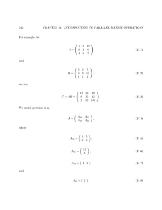
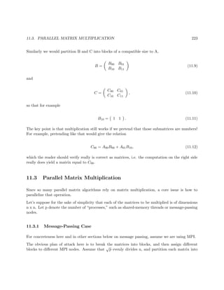
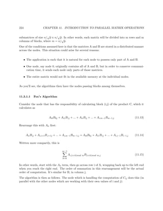
![11.3. PARALLEL MATRIX MULTIPLICATION 225
1 iup = i+1 mod m;
2 idown = i −1 mod m;
3 f o r (k = 0; k < m; k++) {
4 km = ( i+k) mod m;
5 broadcast (A[ i ,km] ) to a l l nodes handling row i of C;
6 C[ i , j ] = C[ i , j ] + A[ i ,km]∗B[km, j ]
7 send B[km, j ] to the node handling C[ idown , j ]
8 r e c e i v e new B[km+1 mod m, j ] from the node handling C[ iup , j ]
9 }
The main idea is to have the various computational nodes repeatedly exchange submatrices with
each other, timed so that a node receives the submatrix it needs for its computation “just in time.”
This is Fox’s algorithm. Cannon’s algorithm is similar, except that it does cyclical rotation in both
rows and columns, compared to Fox’s rotation only in columns but broadcast within rows.
The algorithm can be adapted in the obvious way to nonsquare matrices, etc.
11.3.1.2 Performance Issues
Note that in MPI we would probably want to implement this algorithm using communicators. For
example, this would make broadcasting within a block row more convenient and efficient.
Note too that there is a lot of opportunity here to overlap computation and communication, which
is the best way to solve the communication problem. For instance, we can do the broadcast above
at the same time as we do the computation.
Obviously this algorithm is best suited to settings in which we have PEs in a mesh topology. This
includes hypercubes, though one needs to be a little more careful about communications costs there.
11.3.2 Shared-Memory Case
11.3.2.1 Example: Matrix Multiply in OpenMP
Since a matrix multiplication in serial form consists of nested loops, a natural way to parallelize
the operation in OpenMP is through the for pragma, e.g.
1 #pragma omp p a r a l l e l f o r
2 f o r ( i = 0; i < ncolsa ; i++)
3 f o r ( j = 0; i < nrowsb ; j++) {
4 sum = 0;
5 f o r (k = 0; i < ncolsa ; i++)
6 sum += a [ i ] [ k ] ∗ b [ k ] [ j ] ;
7 }](https://image.slidesharecdn.com/matloff-programmingonparallelmachines-2013-150626072019-lva1-app6892/85/Matloff-programming-on-parallel_machines-2013-245-320.jpg)
![226 CHAPTER 11. INTRODUCTION TO PARALLEL MATRIX OPERATIONS
This would parallelize the outer loop, and we could do so at deeper nesting levels if profitable.
11.3.2.2 Example: Matrix Multiply in CUDA
Given that CUDA tends to work better if we use a large number of threads, a natural choice is for
each thread to compute one element of the product, like this:
1 g l o b a l void matmul( f l o a t ∗ma, f l o a t ∗mb, f l o a t ∗mc, int nrowsa ,
2 int ncolsa , int ncolsb , f l o a t ∗ t o t a l )
3 { int k , i , j ; f l o a t sum ;
4 // find i , j according to thread and block ID
5 sum = 0;
6 f o r (k = 0; k < ncolsa ; k++)
7 sum += a [ i ∗ ncolsa+k ] ∗ b [ k∗ ncols+j ] ;
8 ∗ t o t a l = sum ;
9 }
This should produce a good speedup. But we can do even better, much much better.
The CUBLAS package includes very finely-tuned algorithms for matrix multiplication. The CUBLAS
source code is not public, though, so in order to get an idea of how such tuning might be done,
let’s look at Prof. Richard Edgar’s algorithm, which makes use of shared memory. (Actually, this
may be what CUBLAS uses.)
1 g l o b a l void MultiplyOptimise ( const f l o a t ∗A, const f l o a t ∗B, f l o a t ∗C) {
2 // Extract block and thread numbers
3 int bx = blockIdx . x ; int by = blockIdx . y ;
4 int tx = threadIdx . x ; int ty = threadIdx . y ;
5
6 // Index of f i r s t A sub−matrix processed by t h i s block
7 int aBegin = dc wA ∗ BLOCK SIZE ∗ by ;
8 // Index of l a s t A sub−matrix
9 int aEnd = aBegin + dc wA − 1;
10 // Stepsize of A sub−matrices
11 int aStep = BLOCK SIZE;
12 // Index of f i r s t B sub−matrix
13 // processed by t h i s block
14 int bBegin = BLOCK SIZE ∗ bx ;
15 // Stepsize f o r B sub−matrices
16 int bStep = BLOCK SIZE ∗ dc wB ;
17 // Accumulator f o r t h i s thread
18 f l o a t Csub = 0;
19 f o r ( int a = aBegin , b = bBegin ; a <= aEnd ; a += aStep , b+= bStep ) {
20 // Shared memory f o r sub−matrices
21 s h a r e d f l o a t As [BLOCK SIZE ] [ BLOCK SIZE ] ;
22 s h a r e d f l o a t Bs [BLOCK SIZE ] [ BLOCK SIZE ] ;
23 // Load matrices from global memory into shared memory
24 // Each thread loads one element of each sub−matrix](https://image.slidesharecdn.com/matloff-programmingonparallelmachines-2013-150626072019-lva1-app6892/85/Matloff-programming-on-parallel_machines-2013-246-320.jpg)
![11.3. PARALLEL MATRIX MULTIPLICATION 227
25 As [ ty ] [ tx ] = A[ a + (dc wA ∗ ty ) + tx ] ;
26 Bs [ ty ] [ tx ] = B[ b + (dc wB ∗ ty ) + tx ] ;
27 // Synchronise to make sure load i s complete
28 syncthreads ( ) ;
29 // Perform m u l t i p l i c a t i o n on sub−matrices
30 // Each thread computes one element of the C sub−matrix
31 f o r ( int k = 0; k < BLOCK SIZE; k++ ) {
32 Csub += As [ ty ] [ k ] ∗ Bs [ k ] [ tx ] ;
33 }
34 // Synchronise again
35 syncthreads ( ) ;
36 }
37 // Write the C sub−matrix back to global memory
38 // Each thread writes one element
39 int c = (dc wB ∗ BLOCK SIZE ∗ by) + (BLOCK SIZE∗bx ) ;
40 C[ c + (dc wB∗ty ) + tx ] = Csub ;
41 }
Here are the relevant portions of the calling code, including defined constants giving the number of
columns (“width”) of the multiplier matrix and the number of rows (“height”) of the multiplicand:
1 #define BLOCK SIZE 16
2 . . .
3 c o n s t a n t int dc wA ;
4 c o n s t a n t int dc wB ;
5 . . .
6 // S i z e s must be multiples of BLOCK SIZE
7 dim3 threads (BLOCK SIZE,BLOCK SIZE ) ;
8 dim3 grid (wB/BLOCK SIZE,hA/BLOCK SIZE ) ;
9 MultiplySimple<<<grid , threads >>>(d A , d B , d C ) ;
10 . . .
(Note the alternative way to configure threads, using the functions threads() and grid().)
Here the the term “block” in the defined value BLOCK SIZE refers both to blocks of threads and
the partitioning of matrices. In other words, a thread block consists of 256 threads, to be thought
of as a 16x16 “array” of threads, and each matrix is partitioned into submatrices of size 16x16.
In addition, in terms of grid configuration, there is again a one-to-one correspondence between
thread blocks and submatrices. Each submatrix of the product matrix C will correspond to, and
will be computed by, one block in the grid.
We are computing the matrix product C = AB. Denote the elements of A by aij for the element
in row i, column j, and do the same for B and C. Row-major storage is used.
Each thread will compute one element of C, i.e. one cij. It will do so in the usual way, by multiplying
column j of B by row i of A. However, the key issue is how this is done in concert with the other
threads, and the timing of what portions of A and B are in shared memory at various times.](https://image.slidesharecdn.com/matloff-programmingonparallelmachines-2013-150626072019-lva1-app6892/85/Matloff-programming-on-parallel_machines-2013-247-320.jpg)
![228 CHAPTER 11. INTRODUCTION TO PARALLEL MATRIX OPERATIONS
Concerning the latter, note the code
1 f o r ( int a = aBegin , b = bBegin ; a <= aEnd ; a += aStep , b+= bStep ) {
2 // Shared memory f o r sub−matrices
3 s h a r e d f l o a t As [BLOCK SIZE ] [ BLOCK SIZE ] ;
4 s h a r e d f l o a t Bs [BLOCK SIZE ] [ BLOCK SIZE ] ;
5 // Load matrices from global memory into shared memory
6 // Each thread loads one element of each sub−matrix
7 As [ ty ] [ tx ] = A[ a + (dc wA ∗ ty ) + tx ] ;
8 Bs [ ty ] [ tx ] = B[ b + (dc wB ∗ ty ) + tx ] ;
Here we loop across a row of submatrices of A, and a column of submatrices of B, calculating one
submatrix of C. In each iteration of the loop, we bring into shared memory a new submatrix of
A and a new one of B. Note how even this copying from device global memory to device shared
memory is shared among the threads.
As an example, suppose
A =
1 2 3 4 5 6
7 8 9 10 11 12
(11.16)
and
B =
1 2 3 4
5 6 7 8
9 10 11 12
13 14 15 16
17 18 19 20
21 22 23 24
(11.17)
Further suppose that BLOCK SIZE is 2. That’s too small for good efficiency—giving only four
threads per block rather than 256—but it’s good for the purposes of illustration.
Let’s see what happens when we compute C00, the 2x2 submatrix of C’s upper-left corner. Due to
the fact that partitioned matrices multiply “just like numbers,” we have
C00 = A00B00 + A01B10 + A02B20 (11.18)
=
1 2
7 8
1 2
5 6
+ ... (11.19)
Now, all this will be handled by thread block number (0,0), i.e. the block whose X and Y “coordi-
nates” are both 0. In the first iteration of the loop, A11 and B11 are copied to shared memory for
that block, then in the next iteration, A12 and B21 are brought in, and so on.](https://image.slidesharecdn.com/matloff-programmingonparallelmachines-2013-150626072019-lva1-app6892/85/Matloff-programming-on-parallel_machines-2013-248-320.jpg)
![11.4. FINDING POWERS OF MATRICES 229
Consider what is happening with thread number (1,0) within that block. Remember, its ultimate
goal is to compute c21 (adjusting for the fact that in math, matrix subscripts start at 1). In the
first iteration, this thread is computing
1 2
1
5
= 11 (11.20)
It saves that 11 in its running total Csub, eventually writing it to the corresponding element of C:
int c = (dc wB ∗ BLOCK SIZE ∗ by) + (BLOCK SIZE∗bx ) ;
C[ c + (dc wB∗ty ) + tx ] = Csub ;
Professor Edgar found that use of shared device memory resulted a huge improvement, extending
the original speedup of 20X to 500X!
11.4 Finding Powers of Matrices
In some applications, we are interested not just in multiplying two matrices, but rather in multi-
plying a matrix by itself, many times.
11.4.1 Example: Graph Connectedness
Let n denote the number of vertices in the graph. Define the graph’s adjacency matrix A to be
the n x n matrix whose element (i,j) is equal to 1 if there is an edge connecting vertices i an j (i.e.
i and j are “adjacent”), and 0 otherwise. The corresponding reachability matrix R has its (i,j)
element equal to 1 if there is some path from i to j, and 0 otherwise.
One can prove that
R = b[(I + A)n−1
], (11.21)
where I is the identity matrix and the function b() (‘b’ for “boolean”) is applied elementwise to
its matrix argument, replacing each nonzero element by 1 while leaving the elements which are 0
unchanged. The graph is connected if and only if all elements of R are 1s.
So, the original graph connectivity problem reduces to a matrix problem.](https://image.slidesharecdn.com/matloff-programmingonparallelmachines-2013-150626072019-lva1-app6892/85/Matloff-programming-on-parallel_machines-2013-249-320.jpg)
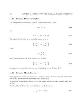
![232 CHAPTER 11. INTRODUCTION TO PARALLEL MATRIX OPERATIONS
As you know, this system can be represented compactly as
Ax = b, (11.32)
where A is n x n and x and b is n x 1.
11.5.1 Gaussian Elimination
Form the n x (n+1) matrix C = (A | b) by appending the column vector b to the right of A. (It
may be advantageous to add padding on the right of b.)
Then we work on the rows of C, with the pseudocode for the sequential case in the most basic
version being
1 f o r i i = 0 to n−1
2 divide row i i by c [ i ] [ i ]
3 f o r r = 0 to n−1, r != i
4 replace row r by row r − c [ r ] [ i i ] times row i i
In the divide operation in the above pseudocode, cii might be 0, or close to 0. In that case, a
pivoting operation is performed (not shown in the pseudocode): that row is first swapped with
another one further down.
This transforms C to reduced row echelon form, in which A is now the identity matrix I and b
is now our solution vector x.
A variation is to transform only to row echelon form. This means that C ends up in upper
triangular form, with all the elements cij with i > j being 0, and with all diagonal elements being
equal to 1. Here is the pseudocode:
1 f o r i i = 0 to n−1
2 divide row i i by c [ i ] [ i ]
3 f o r r = i i +1 to n−1 // vacuous i f r = n−1
4 replace row r by row r − c [ r ] [ i i ] times row i i
This corresponds to a new set of equations,
c00x0 + c11x1 + c22x2 + ... + c0,n−1xn−1 = b0
c11x1 + c22x2 + ... + c1,n−1xn−1 = b1
c22x2 + ... + c2,n−1xn−1 = b2
...
cn−1,n−1xn−1 = bn−1](https://image.slidesharecdn.com/matloff-programmingonparallelmachines-2013-150626072019-lva1-app6892/85/Matloff-programming-on-parallel_machines-2013-252-320.jpg)
![11.5. SOLVING SYSTEMS OF LINEAR EQUATIONS 233
We then find the xi via back substitution:
1 x [ n−1] = b [ n−1] / c [ n−1,n−1]
2 f o r i = n−2 downto 0
3 x [ i ] = (b [ i ] − c [ i ] [ n−1] ∗ x [ n−1] − . . . − c [ i ] [ i +1] ∗ x [ i +1]) / c [ i ] [ i ]
11.5.2 Example: Gaussian Elimination in CUDA
Here’s CUDA code for the reduced row echelon form version, suitable for a not-extremely-large
matrix:
1 // l i n e a r index f o r matrix element at row i , column j , in an m−column
2 // matrix
3 d e v i c e int onedim ( int i , int j , int m) { return i ∗m+j ;}
4
5 // replace u by c∗ u ; vector of length m
6 d e v i c e void cvec ( f l o a t ∗u , int m, f l o a t c )
7 { f o r ( int i = 0; i < m; i++) u [ i ] = c ∗ u [ i ] ; }
8
9 // multiply the vector u of length m by the constant c ( not changing u)
10 // and add the r e s u l t to v
11 d e v i c e void vplscu ( f l o a t ∗u , f l o a t ∗v , int m, f l o a t c )
12 { f o r ( int i = 0; i < m; i++) v [ i ] += c ∗ u [ i ] ; }
13
14 // copy the vector u of length m to v
15 d e v i c e void cpuv ( f l o a t ∗u , f l o a t ∗v , int m)
16 { f o r ( int i = 0; i < m; i++) v [ i ] = u [ i ] ; }
17
18 // solve matrix equation Ax = b ; s t r a i g h t Gaussian elimination , no
19 // pivoting etc . ; the matrix ab i s (A| b ) , n rows ; ab i s destroyed , with
20 // x placed in the l a s t column ; one block , with thread i handling row i
21 g l o b a l void gauss ( f l o a t ∗ab , int n)
22 { int i , n1=n+1, abii , abme ;
23 extern s h a r e d f l o a t iirow [ ] ;
24 int me = threadIdx . x ;
25 f o r ( i = 0; i < n ; i++) {
26 i f ( i == me) {
27 a b i i = onedim ( i , i , n1 ) ;
28 cvec(&ab [ a b i i ] , n1−i ,1/ ab [ a b i i ] ) ;
29 cpuv(&ab [ a b i i ] , iirow , n1−i ) ;
30 }
31 syncthreads ( ) ;
32 i f ( i != me) {
33 abme = onedim (me, i , n1 ) ;
34 vplscu ( iirow ,&ab [ abme ] , n1−i ,−ab [ abme ] ) ;
35 }
36 syncthreads ( ) ;
37 }
38 }](https://image.slidesharecdn.com/matloff-programmingonparallelmachines-2013-150626072019-lva1-app6892/85/Matloff-programming-on-parallel_machines-2013-253-320.jpg)
![234 CHAPTER 11. INTRODUCTION TO PARALLEL MATRIX OPERATIONS
Here we have one thread for each row, and are using just one block, so as to avoid interblock
synchronization problems and to easily use shared memory. Concerning the latter, note that since
the pivot row, iirow, is read many times, it makes sense to put it in shared memory.
Needless to say, the restriction to one block is quite significant. With a 512-thread limit per block,
this would limit us to 512x512 matrices. But it’s even worse than that—if shared memory is only
4K in size, in single precision that would mean something like 30x30 matrices! We could go to
multiple blocks, at the cost of incurring synchronization delays coming from repeated kernel calls.
In a row echelon version of the code, we could have dynamic assignment of rows to threads, but
still would eventually have load balancing issues.
11.5.3 The Jacobi Algorithm
One can rewrite (11.31) as
xi =
1
aii
[bi − (ai0x0 + ... + ai,i−1xi−1 + ai,i+1xi+1 + ... + ai,n−1xn−1)], i = 0, 1, ..., n − 1. (11.33)
This suggests a natural iterative algorithm for solving the equations. We start with our guess
being, say, xi = bi for all i. At our kth iteration, we find our (k+1)st guess by plugging in our kth
guess into the right-hand side of (11.33). We keep iterating until the difference between successive
guesses is small enough to indicate convergence.
This algorithm is guaranteed to converge if each diagonal element of A is larger in absolute value
than the sum of the absolute values of the other elements in its row.
Parallelization of this algorithm is easy: Just assign each process to handle a section of x =
(x0, x1, ..., xn−1). Note that this means that each process must make sure that all other processes
get the new value of its section after every iteration.
Note too that in matrix terms (11.33) can be expressed as
x(k+1)
= D−1
(b − Ox(k)
) (11.34)
where D is the diagonal matrix consisting of the diagonal elements of A (so its inverse is just the
diagonal matrix consisting of the reciprocals of those elements), O is the square matrix obtained by
replacing A’s diagonal elements by 0s, and x(i) is our guess for x in the ithiteration. This reduces
the problem to one of matrix multiplication, and thus we can parallelize the Jacobi algorithm by
utilizing a method for doing parallel matrix multiplication.](https://image.slidesharecdn.com/matloff-programmingonparallelmachines-2013-150626072019-lva1-app6892/85/Matloff-programming-on-parallel_machines-2013-254-320.jpg)
![11.5. SOLVING SYSTEMS OF LINEAR EQUATIONS 235
11.5.4 Example: OpenMP Implementation of the Jacobi Algorithm
OpenMP code for Jacobi is straightforward:
1 #include <omp. h>
2
3 // p a r t i t i o n s s . . e into nc chunks , placing the ith in f i r s t and l a s t ( i
4 // = 0 , . . . , nc−1)
5 void chunker ( int s , int e , int nc , int i , int ∗ f i r s t , int ∗ l a s t )
6 { int chunksize = ( e−s+1) / nc ;
7 ∗ f i r s t = s + i ∗ chunksize ;
8 i f ( i < nc−1) ∗ l a s t = ∗ f i r s t + chunksize − 1;
9 e l s e ∗ l a s t = e ;
10 }
11
12 // returns the ”dot product ” of vectors u and v
13 f l o a t innerprod ( f l o a t ∗u , f l o a t ∗v , int n)
14 { f l o a t sum = 0 . 0 ; int i ;
15 f o r ( i = 0; i < n ; i++)
16 sum += u [ i ] ∗ v [ i ] ;
17 return sum ;
18 }
19
20 // s o l v e s AX = Y, A nxn ; stops i t e r a t i o n when t o t a l change i s < n∗ eps
21 void jacobi ( f l o a t ∗a , f l o a t ∗x , f l o a t ∗y , int n , f l o a t eps )
22 {
23 f l o a t ∗ oldx = malloc (n∗ s i z e o f ( f l o a t ) ) ;
24 f l o a t se ;
25 #pragma omp p a r a l l e l
26 { int i ;
27 int thn = omp get thread num ( ) ;
28 int nth = omp get num threads ( ) ;
29 int f i r s t , l a s t ;
30 chunker (0 ,n−1,nth , thn ,& f i r s t ,& l a s t ) ;
31 f o r ( i = f i r s t ; i <= l a s t ; i++) oldx [ i ] = x [ i ] = 1 . 0 ;
32 f l o a t tmp ;
33 while (1) {
34 f o r ( i = f i r s t ; i <= l a s t ; i++) {
35 tmp = innerprod(&a [ n∗ i ] , oldx , n ) ;
36 tmp −= a [ n∗ i+i ] ∗ oldx [ i ] ;
37 x [ i ] = (y [ i ] − tmp) / a [ n∗ i+i ] ;
38 }
39 #pragma omp b a r r i e r
40 #pragma omp f o r reduction (+: se )
41 f o r ( i = f i r s t ; i <= l a s t ; i++)
42 se += abs (x [ i ]−oldx [ i ] ) ;
43 #pragma omp b a r r i e r
44 i f ( se < n∗ eps ) break ;
45 f o r ( i = f i r s t ; i <= l a s t ; i++)
46 oldx [ i ] = x [ i ] ;](https://image.slidesharecdn.com/matloff-programmingonparallelmachines-2013-150626072019-lva1-app6892/85/Matloff-programming-on-parallel_machines-2013-255-320.jpg)
![238 CHAPTER 11. INTRODUCTION TO PARALLEL MATRIX OPERATIONS
The CULA library for CUDA, mentioned earlier, includes routines for finding the singular value
decomposition of a matrix, thus providing the eigenvectors.1 The R package gputools has an
interface to the SVD routine in CULA.
11.7 Sparse Matrices
As mentioned earlier, in many parallel processing applications of linear algebra, the matrices can
be huge, even having millions of rows or columns. However, in many such cases, most of the matrix
consists of 0s. In an effort to save memory, one can store such matrices in compressed form, storing
only the nonzero elements.
Sparse matrices roughly fall into two categories. In the first category, the matrices all have 0s at
the same known positions. For instance, in tridiagonal matrices, the only nonzero elements are
either on the diagonal or on subdiagonals just below or above the diagonal, and all other elements
are guaranteed to be 0, such as
2 0 0 0 0
1 1 8 0 0
0 1 5 8 0
0 0 0 8 8
0 0 0 3 5
(11.43)
Code to deal with such matrices can then access the nonzero elements based on this knowledge.
In the second category, each matrix that our code handles will typically have its nonzero matrices in
different, “random,” positions. A number of methods have been developed for storing amorphous
sparse matrices, such as the Compressed Sparse Row format, which we’ll code in this C struct,
representing an mxn matrix A, with k nonzero entries:
1 s t r u c t {
2 int m, n ; // numbers of rows and columns of A
3 f l o a t ∗ avals ; // the nonzero values of A, in row−major order ; length k
4 int ∗ c o l s ; // avals [ i ] i s in column c o l s [ i ] in A; length k
5 int ∗ rowplaces ; // rowplaces [ i ] i s the index in avals f o r the 1 st
6 // nonzero element of row i in A ( but l a s t element
7 // i s k ) ; length m+1
8 }
For the matrix in (11.43) (if we were not to exploit its tridiagonal nature, and just treat it as
amorphous):
1
The term singular value is a synonym for eigenvalue.](https://image.slidesharecdn.com/matloff-programmingonparallelmachines-2013-150626072019-lva1-app6892/85/Matloff-programming-on-parallel_machines-2013-258-320.jpg)
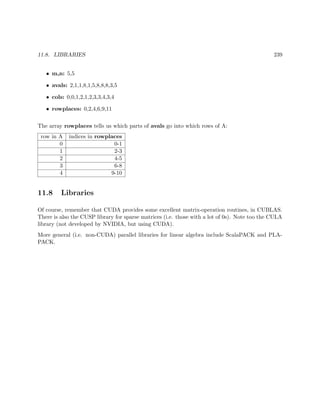

![242 CHAPTER 12. INTRODUCTION TO PARALLEL SORTING
implementation places the two piles back into the original array x. The following C code does that.
The function separate() is intended to be used in a recursive quicksort operation. It operates
on x[l] through x[h], a subarray of x that itself may have been formed at an earlier stage of the
recursion. It forms two piles from those elements, and placing the piles back in the same region
x[l] through x[h]. It also has a return value, showing where the first pile ends.
int separate(int l, int h)
{ int ref,i,j,k,tmp;
ref = x[h]; i = l-1; j = h;
do {
do i++; while (x[i] < ref && i < h);
do j--; while (x[j] > ref && j > l);
tmp = x[i]; x[i] = x[j]; x[j] = tmp;
} while (j > i);
x[j] = x[i]; x[i] = x[h]; x[h] = tmp;
return i;
}
The function separate() rearranges the subarray, returning a value m, so that:
• x[l] through x[m-1] are less than x[m],
• x[m+1] through x[h] are greater than x[m], and
• x[m] is in its “final resting place,” meaning that x[m] will never move again for the remainder
of the sorting process. (Another way of saying this is that the current x[m] is the m-th
smallest of all the original x[i], i = 0,1,...,n-1.)
By the way, x[l] through x[m-1] will also be in their final resting places as a group. They may be
exchanging places with each other from now on, but they will never again leave the range i though
m-1 within the x array as a whole. A similar statement holds for x[m+1] through x[n-1].
Another approach is to do a prefix scan. As an illustration, consider the array
28 35 12 5 13 6 8 10 168 (12.1)
We’ll take the first element, 28, as the pivot, and form a new array of 1s and 0s, where 1 means
“less than the pivot”:
28 35 12 5 13 6 48 10 168
1 0 1 1 1 1 0 1 0
Now form the prefix scan (Chapter 10) of that second array, with respect to addition. It will be an
exclusive scan (Section 10.3). This gives us](https://image.slidesharecdn.com/matloff-programmingonparallelmachines-2013-150626072019-lva1-app6892/85/Matloff-programming-on-parallel_machines-2013-262-320.jpg)
![12.1. QUICKSORT 243
28 35 12 5 13 6 48 10 168
0 0 1 1 1 1 0 1 0
0 0 0 1 2 3 3 4 4
Now, the key point is that for every element 1 in that second row, the corresponding element in
the third row shows where the first-row element should be placed under the separation operation!
Here’s why:
The elements 12, 5, 13, 6 and 10 should go in the first pile, which in an in-place separation would
means indices 0, 1, 2, 3, and 4. Well, as you can see above, these are precisely the values shown in
the third row for 12, 5, 13, 6 and 10, all of which have 1s in the second row.
The pivot, 28, then should immediately follow that low pile, i.e. it should be placed at index 5.
We can simply place the high pile at the remaining indicies, 6 through 8 (though we’ll do it more
systematically below).
In general for an array of length k, we:
• form the second row of 1s and 0s indicating < pivot
• form the third row, the exclusive prefix scan
• for each 1 in the second row, place the corresponding element in row 1 into the spot indicated
by row 3
• place the pivot in the place indicated by 1 plus m, the largest value in row 3
• form row 4, equal to (0,1,...,k-1) minus row 3 plus m
• for each 0 in the second row, place the corresponding element in row 1 into the spot indicated
by row 4
Note that this operation, using scan, could be used an an alternative to the separate() function
above. But it could be done in parallel; more on this below.
12.1.2 Example: OpenMP Quicksort
Here is OpenMP code which performs quicksort in the shared-memory paradigm (adapted from
code in the OpenMP Source Code Repository, http://www.pcg.ull.es/ompscr/):
1 void qs(int *x, int l, int h)
2 { int newl[2], newh[2], i, m;
3 m = separate(x,l,h);
4 newl[0] = l; newh[0] = m-1;](https://image.slidesharecdn.com/matloff-programmingonparallelmachines-2013-150626072019-lva1-app6892/85/Matloff-programming-on-parallel_machines-2013-263-320.jpg)
![244 CHAPTER 12. INTRODUCTION TO PARALLEL SORTING
5 newl[1] = m+1; newh[1] = h;
6 #pragma omp parallel
7 {
8 #pragma omp for nowait
9 for (i = 0; i < 2; i++)
10 qs(newl[i],newh[i]);
11 }
12 }
Note the nowait clause. Since different threads are operating on different portions of the array,
they need not be synchronized.
Recall that another implementation, using the task directive, was given earlier in Section 4.5.
In both of these implementations, we used the function separate() defined above. So, different
threads apply different separation operations to different subarrays. An alternative would be to
place the parallelism in the separation operation itself, using the parallel algorithms for prefix scan
in Chapter 10.
12.1.3 Hyperquicksort
This algorithm was originally developed for hypercubes, but can be used on any message-passing
system having a power of 2 for the number of nodes.1
It is assumed that at the beginning each PE contains some chunk of the array to be sorted. After
sorting, each PE will contain some chunk of the sorted array, meaning that:
• each chunk is itself in sorted form
• for all cases of i < j, the elements at PE i are less than the elements at PE j
If the sorted array itself were our end, rather than our means to something else, we could now
collect it at some node, say node 0. If, as is more likely, the sorting is merely an intermediate step
in a larger distributed computation, we may just leave the chunks at the nodes and go to the next
phase of work.
Say we are on a d-cube. The intuition behind the algorithm is quite simple:
for i = d downto 1
for each i-cube:
root of the i-cube broadcasts its median to all in the i-cube,
to serve as pivot
consider the two (i-1)-subcubes of this i-cube
1
See Chapter 7 for definitions of hypercube terms.](https://image.slidesharecdn.com/matloff-programmingonparallelmachines-2013-150626072019-lva1-app6892/85/Matloff-programming-on-parallel_machines-2013-264-320.jpg)
![248 CHAPTER 12. INTRODUCTION TO PARALLEL SORTING
• Each of the pairs (ai, ai+1), i = 0,2,...,n-2 is bitonic, since any 2-element array is bitonic!
• Apply sortbitonic() to (ai, ai+1). In this case, we are simply doing a compare-exchange.
• If i/2 is odd, reverse the pair, so that this pair and the pair immediately preceding it
now form a 4-element bitonic sequence.
2. For each i = 0,4,8,...,n-4:
• Apply sortbitonic() to (ai, ai+1, ai+2, ai+3).
• If i/4 is odd, reverse the quartet, so that this quartet and the quartet immediately
preceding it now form an 8-element bitonic sequence.
3. Keep building in this manner, until get to a single sorted n-element list.
There are many ways to parallelize this. In the hypercube case, the algorithm consists of doing
compare-exchange operations with all neighbors, pretty much in the same pattern as hyperquicksort.
12.3 The Bubble Sort and Its Cousins
12.3.1 The Much-Maligned Bubble Sort
Recall the bubble sort:
1 void bubblesort(int *x, int n)
2 { for i = n-1 downto 1
3 for j = 0 to i
4 compare-exchange(x,i,j,n)
5 }
Here the function compare-exchange() is as in Section 12.2.4 above. In the context here, it boils
down to
if x[i] > x[j]
swap x[i] and x[j]
In the first i iteration, the largest element “bubbles” all the way to the right end of the array. In
the second iteration, the second-largest element bubbles to the next-to-right-end position, and so
on.
You learned in your algorithms class that this is a very inefficient algorithm—when used serially.
But it’s actually rather usable in parallel systems.](https://image.slidesharecdn.com/matloff-programmingonparallelmachines-2013-150626072019-lva1-app6892/85/Matloff-programming-on-parallel_machines-2013-268-320.jpg)
![12.3. THE BUBBLE SORT AND ITS COUSINS 249
For example, in the shared-memory setting, suppose we have one thread for each value of i. Then
those threads can work in parallel, as long as a thread with a larger value of i does not overtake a
thread with a smaller i, where “overtake” means working on a larger j value.
Once again, it probably pays to chunk the data. In this case, compare-exchange() fully takes on
the meaning it had in Section 12.2.4.
12.3.2 A Popular Variant: Odd-Even Transposition
A popular variant of this is the odd-even transposition sort. The pseudocode for a shared-
memory version is:
1 // the argument "me" is this thread’s ID
2 void oddevensort(int *x, int n, int me)
3 { for i = 1 to n
4 if i is odd
5 if me is even
6 compare-exchange(x,me,me+1,n)
7 else // me is odd
8 compare-exchange(x,me,me-1,n)
9 else // i is even
10 if me is even
11 compare-exchange(x,me,me-1,n)
12 else // me is odd
13 compare-exchange(x,me,me+1,n)
If the second or third argument of compare-exchange() is less than 0 or greater than n-1, the
function has no action.
This looks a bit complicated, but all it’s saying is that, from the point of view of an even-numbered
element of x, it trades with its right neighbor during odd phases of the procedure and with its left
neighbor during even phases.
Again, this is usually much more effective if done in chunks.
12.3.3 Example: CUDA Implementation of Odd/Even Transposition Sort
1 #include <stdio.h>
2 #include <stdlib.h>
3 #include <cuda.h>
4
5 // compare and swap; copies from the f to t, swapping f[i] and
6 // f[j] if the higher-index value is smaller; it is required that i < j
7 __device__ void cas(int *f,int *t,int i,int j, int n, int me)
8 {
9 if (i < 0 || j >= n) return;
10 if (me == i) {](https://image.slidesharecdn.com/matloff-programmingonparallelmachines-2013-150626072019-lva1-app6892/85/Matloff-programming-on-parallel_machines-2013-269-320.jpg)
![250 CHAPTER 12. INTRODUCTION TO PARALLEL SORTING
11 if (f[i] > f[j]) t[me] = f[j];
12 else t[me] = f[i];
13 } else { // me == j
14 if (f[i] > f[j]) t[me] = f[i];
15 else t[me] = f[j];
16 }
17 }
18
19 // does one iteration of the sort
20 __global__ void oekern(int *da, int *daaux, int n, int iter)
21 { int bix = blockIdx.x; // block number within grid
22 if (iter % 2) {
23 if (bix % 2) cas(da,daaux,bix-1,bix,n,bix);
24 else cas(da,daaux,bix,bix+1,n,bix);
25 } else {
26 if (bix % 2) cas(da,daaux,bix,bix+1,n,bix);
27 else cas(da,daaux,bix-1,bix,n,bix);
28 }
29 }
30
31 // sorts the array ha, length n, using odd/even transp. sort;
32 // kept simple for illustration, no optimization
33 void oddeven(int *ha, int n)
34 {
35 int *da;
36 int dasize = n * sizeof(int);
37 cudaMalloc((void **)&da,dasize);
38 cudaMemcpy(da,ha,dasize,cudaMemcpyHostToDevice);
39 // the array daaux will serve as "scratch space"
40 int *daaux;
41 cudaMalloc((void **)&daaux,dasize);
42 dim3 dimGrid(n,1);
43 dim3 dimBlock(1,1,1);
44 int *tmp;
45 for (int iter = 1; iter <= n; iter++) {
46 oekern<<<dimGrid,dimBlock>>>(da,daaux,n,iter);
47 cudaThreadSynchronize();
48 if (iter < n) {
49 // swap pointers
50 tmp = da;
51 da = daaux;
52 daaux = tmp;
53 } else
54 cudaMemcpy(ha,daaux,dasize,cudaMemcpyDeviceToHost);
55 }
56 }
Recall that in CUDA code, separate blocks of threads cannot synchronize with each other. Unless
we deal with just a single block, this necessitates limiting the kernel to a single iteration of the
algorithm, so that as iterations progress, execution alternates between the device and the host.
Moreover, we do not take advantage of shared memory. One possible solution would be to use
syncthreads() within each block for most of the compare-and-exchange operations, and then
having the host take care of the operations on the boundaries between blocks.](https://image.slidesharecdn.com/matloff-programmingonparallelmachines-2013-150626072019-lva1-app6892/85/Matloff-programming-on-parallel_machines-2013-270-320.jpg)
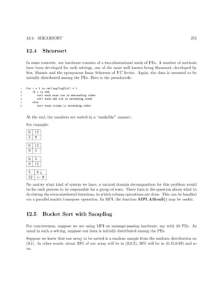
![252 CHAPTER 12. INTRODUCTION TO PARALLEL SORTING
What we could do is assign PE0 to the interval (0,0.1), PE1 to (0.1,0.2) etc. Each PE would look
at its local data, and distribute it to the other PEs according to this interval scheme. Then each
PE would do a local sort.
In general, we don’t know what distribution our data comes from. We solve this problem by doing
sampling. In our example here, each PE would sample some of its local data, and send the sample
to PE0. From all of these samples, PE0 would find the decile values, i.e. 10th percentile, 20th
percentile,..., 90th percentile. These values, called splitters would then be broadcast to all the
PEs, and they would then distribute their local data to the other PEs according to these intervals.
OpenMP code for this was given in Section 1.3.2.6. Here is similar MPI code below (various
improvements could be made, e.g. with broadcast):
1 // bucket sort , bin boundaries known in advance
2
3 // node 0 i s manager , a l l e l s e worker nodes ; node 0 sends f u l l data , bin
4 // boundaries to a l l worker nodes ; i−th worker node ex t ra c ts data f o r
5 // bin i −1, s o r t s it , sends sorted chunk back to node 0; node 0 places
6 // sorted r e s u l t s back in o r i g i n a l array
7
8 // not claimed e f f i c i e n t ; e . g . could be better to have manager place
9 // items into bins
10
11 #include <mpi . h>
12
13 #define MAX N 100000 // max s i z e of o r i g i n a l data array
14 #define MAX NPROCS 100 // max number of MPI processes
15 #define DATA MSG 0 // manager sending o r i g i n a l data
16 #define BDRIES MSG 0 // manager sending bin boundaries
17 #define CHUNKS MSG 2 // workers sending t h e i r sorted chunks
18
19 int nnodes , //
20 n , // s i z e of f u l l array
21 me, // my node number
22 f u l l d a t a [MAX N] ,
23 tmp [MAX N] ,
24 nbdries , // number of bin boundaries
25 counts [MAX NPROCS] ;
26 f l o a t bdries [MAX NPROCS−2]; // bin boundaries
27
28 int debug , debugme ;
29
30 i n i t ( int argc , char ∗∗ argv )
31 {
32 int i ;
33 debug = at o i ( argv [ 3 ] ) ;
34 debugme = a t o i ( argv [ 4 ] ) ;
35 MPI Init(&argc ,&argv ) ;
36 MPI Comm size (MPI COMM WORLD,&nnodes ) ;](https://image.slidesharecdn.com/matloff-programmingonparallelmachines-2013-150626072019-lva1-app6892/85/Matloff-programming-on-parallel_machines-2013-272-320.jpg)
![12.5. BUCKET SORT WITH SAMPLING 253
37 MPI Comm rank(MPI COMM WORLD,&me ) ;
38 nbdries = nnodes − 2;
39 n = a t oi ( argv [ 1 ] ) ;
40 int k = a t oi ( argv [ 2 ] ) ; // f o r random # gen
41 // generate random data f o r t e s t purposes
42 f o r ( i = 0; i < n ; i++) f u l l d a t a [ i ] = rand () % k ;
43 // generate bin boundaries f o r t e s t purposes
44 f o r ( i = 0; i < nbdries ; i++) {
45 bdries [ i ] = i ∗ (k+1) / (( f l o a t ) nnodes ) ;
46 }
47 }
48
49 void managernode ()
50 {
51 MPI Status status ;
52 int i ;
53 int lenchunk ; // length of a chunk received from a worker
54 // send f u l l data , bin boundaries to workers
55 f o r ( i = 1; i < nnodes ; i++) {
56 MPI Send ( fulldata , n , MPI INT , i ,DATA MSG,MPI COMM WORLD) ;
57 MPI Send ( bdries , nbdries ,MPI FLOAT, i ,BDRIES MSG,MPI COMM WORLD) ;
58 }
59 // c o l l e c t sorted chunks from workers , place them in t h e i r proper
60 // p o s i t i o n s within the o r i g i n a l array
61 int c u r r p o s i t i o n = 0;
62 f o r ( i = 1; i < nnodes ; i++) {
63 MPI Recv(tmp ,MAX N, MPI INT , i ,CHUNKS MSG,MPI COMM WORLD,& status ) ;
64 MPI Get count(&status , MPI INT,& lenchunk ) ;
65 memcpy( f u l l d a t a+currposition , tmp , lenchunk ∗ s i z e o f ( int ) ) ;
66 c u r r p o s i t i o n += lenchunk ;
67 }
68 i f (n < 25) {
69 f o r ( i = 0; i < n ; i++) p r i n t f (”%d ” , f u l l d a t a [ i ] ) ;
70 p r i n t f (”n ” ) ;
71 }
72 }
73
74 // adds xi to the part array , increments npart , the length of part
75 void grab ( int xi , int ∗part , int ∗ npart )
76 {
77 part [∗ npart ] = xi ;
78 ∗ npart += 1;
79 }
80
81 int cmpints ( int ∗u , int ∗v)
82 { i f (∗u < ∗v) return −1;
83 i f (∗u > ∗v) return 1;
84 return 0;
85 }
86](https://image.slidesharecdn.com/matloff-programmingonparallelmachines-2013-150626072019-lva1-app6892/85/Matloff-programming-on-parallel_machines-2013-273-320.jpg)
![254 CHAPTER 12. INTRODUCTION TO PARALLEL SORTING
87 void getandsortmychunk ( int ∗tmp , int n , int ∗chunk , int ∗ lenchunk )
88 {
89 int i , count = 0;
90 int workernumber = me − 1;
91 i f (me == debugme) while ( debug ) ;
92 f o r ( i = 0; i < n ; i++) {
93 i f ( workernumber == 0) {
94 i f (tmp [ i ] <= bdries [ 0 ] ) grab (tmp [ i ] , chunk ,&count ) ;
95 }
96 e l s e i f ( workernumber < nbdries −1) {
97 i f (tmp [ i ] > bdries [ workernumber −1] &&
98 tmp [ i ] <= bdries [ workernumber ] ) grab (tmp [ i ] , chunk ,&count ) ;
99 } e l s e
100 i f (tmp [ i ] > bdries [ nbdries −1]) grab (tmp [ i ] , chunk ,&count ) ;
101 }
102 qsort ( chunk , count , s i z e o f ( int ) , cmpints ) ;
103 ∗ lenchunk = count ;
104 }
105
106 void workernode ()
107 {
108 int n , f u l l d a t a [MAX N] , // s i z e and storage of f u l l data
109 chunk [MAX N] ,
110 lenchunk ,
111 nbdries ; // number of bin boundaries
112 f l o a t bdries [MAX NPROCS−1]; // bin boundaries
113 MPI Status status ;
114 MPI Recv( fulldata ,MAX N, MPI INT , 0 ,DATA MSG,MPI COMM WORLD,& status ) ;
115 MPI Get count(&status , MPI INT,&n ) ;
116 MPI Recv( bdries ,MAX NPROCS−2,MPI FLOAT, 0 ,BDRIES MSG,MPI COMM WORLD,& status ) ;
117 MPI Get count(&status ,MPI FLOAT,& nbdries ) ;
118 getandsortmychunk ( fulldata , n , chunk ,&lenchunk ) ;
119 MPI Send ( chunk , lenchunk , MPI INT , 0 ,CHUNKS MSG,MPI COMM WORLD) ;
120 }
121
122 int main ( int argc , char ∗∗ argv )
123 {
124 int i ;
125 i n i t ( argc , argv ) ;
126 i f (me == 0) managernode ( ) ;
127 e l s e workernode ( ) ;
128 MPI Finalize ( ) ;
129 }](https://image.slidesharecdn.com/matloff-programmingonparallelmachines-2013-150626072019-lva1-app6892/85/Matloff-programming-on-parallel_machines-2013-274-320.jpg)
![12.6. RADIX SORT 255
12.6 Radix Sort
The radix sort is essentially a special case of a bucket sort. If we have 16 threads, say, we could
determine a datum’s bucket by its lower 4 bits. As long as our data is uniformly distributed under
the mod 16 operation, we would not need to do any sampling.
The CUDPP GPU library uses a radix sort. The buckets are formed one bit at a time, using
segmented scan as above.
12.7 Enumeration Sort
This one is really simple. Take for instance the array (12,5,13,18,6). There are 2 elements less than
12, so in the end, it should go in position 2 of the sorted array, (5,6,12,13,18).
Say we wish to sort x, which for convenience we assume contains no tied values. Then the pseu-
docode for this algorithm, placing the results in y, is
for all i in 0...n-1:
count = 0
elt = x[i]
for all j in 0...n-1:
if x[j] < elt then count++
y[count] = elt
The outer (or inner) loop is easily parallelized.](https://image.slidesharecdn.com/matloff-programmingonparallelmachines-2013-150626072019-lva1-app6892/85/Matloff-programming-on-parallel_machines-2013-275-320.jpg)

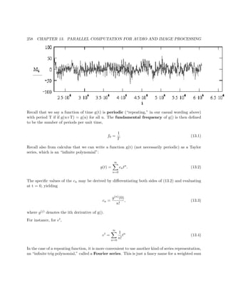
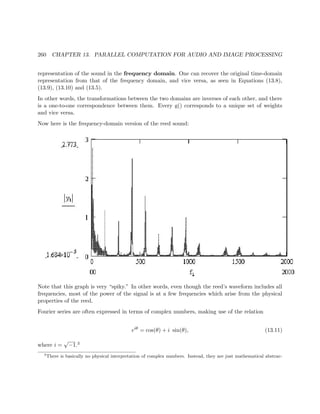
![13.2. DISCRETE FOURIER TRANSFORMS 263
where X is the vector xj and
A =
1 1 1 ... 1
1 q q2 ... qn−1
... ... ... ... ...
1 qn−1 q2(n−1) ... q(n−1)(n−1)
(13.17)
Here’s R code to calculate A:
1 makeamat <- function(n,u) {
2 m <- matrix(nrow=n,ncol=n)
3 for (i in 1:n) {
4 for (j in i:n) {
5 if (i == j) {
6 m[i,i] <- u^((i-1)^2)
7 }
8 else {
9 m[i,j] <- u^((i-1)*(j-1))
10 m[j,i] <- m[i,j]
11 }
12 }
13 }
14 m
15 }
13.2.2 Inversion
As in the continuous case, the DFT is a one-to-one transformation. so we can recover each domain
from the other. The details are important:
The matrix A in (13.17) is a special case of Vandermonde matrices, known to be invertible. In
fact, if we think of that matrix as a function of q, A(q), then it turns out that
[A(q)]−1
=
1
n
A(
1
q
) (13.18)
Thus (13.16) becomes
X = n[A(q)]−1
C = A(
1
q
)C (13.19)](https://image.slidesharecdn.com/matloff-programmingonparallelmachines-2013-150626072019-lva1-app6892/85/Matloff-programming-on-parallel_machines-2013-283-320.jpg)
![264 CHAPTER 13. PARALLEL COMPUTATION FOR AUDIO AND IMAGE PROCESSING
In nonmatrix terms:
xj =
n−1
k=0
cke2πijk/n
=
n−1
k=0
ckq−jk
(13.20)
Equation (13.20) is basically a discrete analog of (13.5).
13.2.2.1 Alternate Formulation
Equation (13.16) has a factor 1/n while (13.19) doesn’t. In order to achieve symmetry, some authors
of material on DFT opt to define the DFT and its inverse with 1/
√
n in (13.13) instead of 1/n, and
by adding a factor 1/
√
n in (13.20). They then include a factor 1/
√
n in (13.17), with the result
that [A(q)]−1 = A(1/q). Thus everything simplifies.
Other formulations are possible. For instance, the R fft() routine’s documentation says it’s “unnor-
malized,” meaning that there is neither a 1/n nor a 1/
√
n in (13.20). When using a DFT routine,
be sure to determine what it assumes about these constant factors.
13.2.3 Two-Dimensional Data
The spectrum numbers crs are double-subscripted, like the original data xuv, the latter being the
pixel intensity in row u, column v of the image, u = 0,1,...,n-1, v = 0,1,...,m-1. Equation (13.13)
becomes
crs =
1
n
1
m
n−1
j=0
m−1
k=0
xjke−2πi( jr
n
+ks
m
)
(13.21)
where r = 0,1,...,n-1, s = 0,1,...,m-1.
Its inverse is
xrs =
n−1
j=0
m−1
k=0
cjke2πi(jr
n
+ks
m
)
(13.22)](https://image.slidesharecdn.com/matloff-programmingonparallelmachines-2013-150626072019-lva1-app6892/85/Matloff-programming-on-parallel_machines-2013-284-320.jpg)
![268 CHAPTER 13. PARALLEL COMPUTATION FOR AUDIO AND IMAGE PROCESSING
13.5 Applications to Image Processing
In image processing, there are a number of different operations which we wish to perform. We will
consider two of them here.
13.5.1 Smoothing
An image may be too “rough.” There may be some pixels which are noise, accidental values that
don’t fit smoothly with the neighboring points in the image.
One way to smooth things out would be to replace each pixel intensity value7 by the mean or
median among the pixels neighbors. These could be the four immediate neighbors if just a little
smoothing is needed, or we could go further out for a higher amount of smoothing. There are many
variants of this.
But another way would be to apply a low-pass filter to the DFT of our image. This means that
after we compute the DFT, we simply delete the higher harmonics, i.e. set crs to 0 for the larger
values of r and s. We then take the inverse transform back to the spatial domain. Remember, the
sine and cosine functions of higher harmonics are “wigglier,” so you can see that all this will have
the effect of removing some of the wiggliness in our image—exactly what we wanted.
We can control the amount of smoothing by the number of harmonics we remove.
The term low-pass filter obviously alludes to the fact that the low frequencies “pass” through the
filter but the high frequencies are blocked. Since we’ve removed the high-oscillatory components,
the effect is a smoother image.8
To do smoothing in parallel, if we just average neighbors, this is easily parallelized. If we try a
low-pass filter, then we use the parallelization methods shown here earlier.
13.5.2 Example: Audio Smoothing in R
Below is code to do smoothing on sound. It inputs a sound sequence snd, and performs low-pass
filtering, setting to 0 all DFT terms having k greater than maxidx in (13.13).
1 p <- function(snd,maxidx) {
2 four <- fft(snd)
3 n <- length(four)
4 newfour <- c(four[1:maxidx],rep(0,n-maxidx))
5 return(Re(fft(newfour,inverse=T)/n))
6 }
7
Remember, there may be three intensity values per pixel, for red, green and blue.
8
Note that we may do more smoothing in some parts of the image than in others.](https://image.slidesharecdn.com/matloff-programmingonparallelmachines-2013-150626072019-lva1-app6892/85/Matloff-programming-on-parallel_machines-2013-288-320.jpg)
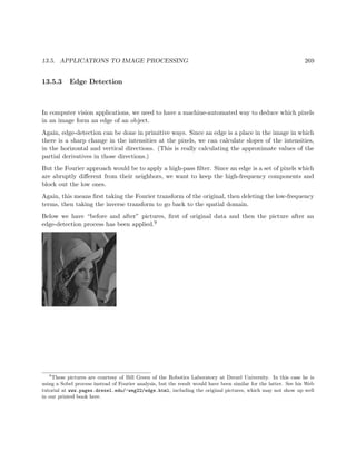
![13.8. DOES THE FUNCTION G() REALLY HAVE TO BE REPEATING? 271
13.8 Does the Function g() Really Have to Be Repeating?
It is clear that in the case of a vibrating reed, our loudness function g(t) really is periodic. What
about other cases?
A graph of your voice would look “locally periodic.” One difference would be that the graph would
exhibit more change through time as you make various sounds in speaking, compared to the one
repeating sound for the reed. Even in this case, though, your voice is repeating within short time
intervals, each interval corresponding to a different sound. If you say the word eye, for instance, you
make an “ah” sound and then an “ee” sound. The graph of your voice would show one repeating
pattern during the time you are saying “ah,” and another repeating pattern during the time you
are saying “ee.” So, even for voices, we do have repeating patterns over short time intervals.
On the other hand, in the image case, the function may be nearly constant for long distances
(horizontally or vertically), so a local periodicity argument doesn’t seem to work there.
The fact is, though, that it really doesn’t matter in the applications we are considering here. Even
though mathematically our work here has tacitly assumed that our image is duplicated infinitely
times (horizontally and vertically),10 we don’t care about this. We just want to get a measure of
“wiggliness,” and fitting linear combinations of trig functions does this for us.
13.9 Vector Space Issues (optional section)
The theory of Fourier series (and of other similar transforms), relies on vector spaces. It actually
is helpful to look at some of that here. Let’s first discuss the derivation of (13.13).
Define X and C as in Section 13.2. X’s components are real, but it is also a member of the vector
space V of all n-component arrays of complex numbers.
For any complex number a+bi, define its conjugate, a + bi = a − bi. Note that
eiθ = cos θ − i sin θ == cos(−θ) + i sin(−θ) = e−iθ
(13.28)
Define an inner product (“dot product”),
[u, w] =
1
n
n−1
j=0
uj ¯wj. (13.29)
10
And in the case of the cosine transform, implicitly we are assuming that the image flips itself on every adjacent
copy of the image, first right-side up, then upside-own, then right-side up again, etc.](https://image.slidesharecdn.com/matloff-programmingonparallelmachines-2013-150626072019-lva1-app6892/85/Matloff-programming-on-parallel_machines-2013-291-320.jpg)
![272 CHAPTER 13. PARALLEL COMPUTATION FOR AUDIO AND IMAGE PROCESSING
Define
vh = (1, q−h
, q−2h
, ..., q−(n−1)h
), h = 0, 1, ..., n − 1. (13.30)
Then it turns out that the vh form an orthonormal basis for V.11 For example, to show orthnogo-
nality, observe that for r = s
[vr, vs] =
1
n
n−1
j=0
vrjvsj (13.31)
=
1
n
j=0
qj(−r+s)
(13.32)
=
1 − q(−r+s)n
n(1 − q)
(13.33)
= 0, (13.34)
due to the identity 1 + y + y2 + .... + yk = 1−yk+1
1−y and the fact that qn = 1. In the case r = s, the
above computation shows that [vr, vs] = 1.
The DFT of X, which we called C, can be considered the “coordinates” of X in V, relative to this
orthonormal basis. The kth coordinate is then [X, vk], which by definition is (13.13).
The fact that we have an orthonormal basis for V here means that the matrix A/n in (13.25) is
an orthogonal matrix. For real numbers, this means that this matrix’s inverse is its transpose. In
the complex case, instead of a straight transpose, we do a conjugate transpose, B = A/n
t
, where t
means transpose. So, B is the inverse of A/n. In other words, in (13.25), we can easily get back to
X from C, via
X = BC =
1
n
¯At
C. (13.35)
It’s really the same for the nondiscrete case. Here the vector space consists of all the possible
periodic functions g() (with reasonable conditions placed regarding continuity etc.) forms the
vector space, and the sine and cosine functions form an orthonormal basis. The an and bn are then
the “coordinates” of g() when the latter is viewed as an element of that space.
11
Recall that this means that these vectors are orthogonal to each other, and have length 1, and that they span V.](https://image.slidesharecdn.com/matloff-programmingonparallelmachines-2013-150626072019-lva1-app6892/85/Matloff-programming-on-parallel_machines-2013-292-320.jpg)
![13.10. BANDWIDTH: HOW TO READ THE SAN FRANCISCO CHRONICLE BUSINESS PAGE (OPTIONAL S
13.10 Bandwidth: How to Read the San Francisco Chronicle
Business Page (optional section)
The popular press, especially business or technical sections, often uses the term bandwidth. What
does this mean?
Any transmission medium has a natural range [fmin,fmax] of frequencies that it can handle well.
For example, an ordinary voice-grade telephone line can do a good job of transmitting signals
of frequencies in the range 0 Hz to 4000 Hz, where “Hz” means cycles per second. Signals of
frequencies outside this range suffer fade in strength, i.e are attenuated, as they pass through the
phone line.12
We call the frequency interval [0,4000] the effective bandwidth (or just the bandwidth) of the
phone line.
In addition to the bandwidth of a medium, we also speak of the bandwidth of a signal. For
instance, although your voice is a mixture of many different frequencies, represented in the Fourier
series for your voice’s waveform, the really low and really high frequency components, outside the
range [340,3400], have very low power, i.e. their an and bn coefficients are small. Most of the power
of your voice signal is in that range of frequencies, which we would call the effective bandwidth
of your voice waveform. This is also the reason why digitized speech is sampled at the rate of
8,000 samples per second. A famous theorem, due to Nyquist, shows that the sampling rate should
be double the maximum frequency. Here the number 3,400 is “rounded up” to 4,000, and after
doubling we get 8,000.
Obviously, in order for your voice to be heard well on the other end of your phone connection, the
bandwidth of the phone line must be at least as broad as that of your voice signal, and that is the
case.
However, the phone line’s bandwidth is not much broader than that of your voice signal. So, some
of the frequencies in your voice will fade out before they reach the other person, and thus some
degree of distortion will occur. It is common, for example, for the letter ‘f’ spoken on one end to be
mis-heard as ‘s’on the other end. This also explains why your voice sounds a little different on the
phone than in person. Still, most frequencies are reproduced well and phone conversations work
well.
We often use the term “bandwidth” to literally refer to width, i.e. the width of the interval
[fmin, fmax].
There is huge variation in bandwidth among transmission media. As we have seen, phone lines
have bandwidth intervals covering values on the order of 103. For optical fibers, these numbers are
more on the order of 1015.
12
And in fact will probably be deliberately filtered out.](https://image.slidesharecdn.com/matloff-programmingonparallelmachines-2013-150626072019-lva1-app6892/85/Matloff-programming-on-parallel_machines-2013-293-320.jpg)
![274 CHAPTER 13. PARALLEL COMPUTATION FOR AUDIO AND IMAGE PROCESSING
The radio and TV frequency ranges are large also, which is why, for example, we can have many AM
radio stations in a given city. The AM frequency range is divided into subranges, called channels.
The width of these channels is on the order of the 4000 we need for a voice conversation. That
means that the transmitter at a station needs to shift its content, which is something like in the
[0,4000] range, to its channel range. It does that by multiplying its content times a sine wave of
frequency equal to the center of the channel. If one applies a few trig identities, one finds that the
product signal falls into the proper channel!
Accordingly, an optical fiber could also carry many simultaneous phone conversations.
Bandwidth also determines how fast we can set digital bits. Think of sending the sequence
10101010... If we graph this over time, we get a “squarewave” shape. Since it is repeating, it
has a Fourier series. What happends if we double the bit rate? We get the same graph, only hori-
zontally compressed by a factor of two. The effect of this on this graph’s Fourier series is that, for
example, our former a3 will now be our new a6, i.e. the 2π · 3f0 frequency cosine wave component
of the graph now has the double the old frequency, i.e. is now 2π · 6f0. That in turn means that
the effective bandwidth of our 10101010... signal has doubled too.
In other words: To send high bit rates, we need media with large bandwidths.](https://image.slidesharecdn.com/matloff-programmingonparallelmachines-2013-150626072019-lva1-app6892/85/Matloff-programming-on-parallel_machines-2013-294-320.jpg)
![14.2. PROBABILITY DENSITY ESTIMATION 279
14.2.1 Kernel-Based Density Estimation
Histogram computation breaks the real down into intervals, and then counts how many Xi fall into
each interval. This is fine as a crude method, but one can do better.
No matter what the interval width is, the histogram will consist of a bunch of rectanges, rather
than a smooth curve. This problem basically stems from a lack of weighting on the data.
For example, suppose we are estimating f(25.8), and suppose our histogram interval is [24.0,26.0],
with 54 points falling into that interval. Intuitively, we can do better if we give the points closer
to 25.8 more weight.
One way to do this is called kernel-based density estimation, which for instance in R is handled
by the function density().
We need a set of weights, more precisely a weight function k, called the kernel. Any nonnegative
function which integrates to 1—i.e. a density function in its own right—will work. Typically k is
taken to be the Gaussian or normal density function,
k(u) =
1
√
2π
e−0.5u2
(14.2)
Our estimator is then
f(t) =
1
nh
n
i=1
k
t − Xi
h
(14.3)
In statistics, it is customary to use the symbol (pronounced “hat”) to mean “estimate of.” Here
f means the estimate of f.
Note carefully that we are estimating an entire function! There are infinitely many possible values
of t, thus infinitely many values of f(t) to be estimated. This is reflected in (14.3), as f(t) does
indeed give a (potentially) different value for each t.
Here h, called the bandwidth, is playing a role analogous to the interval width in the case of
histograms. We must choose the value of h, just like for a histogram we must choose the bin
width.3
Again, this looks very abstract, but all it is doing is assigning weights to the data. Consider our
example above in which we wish to estimate f(25.8), i.e. t = 25.8 and suppose we choose h to be
6.0. If say, X88 is 1209.1, very far as away from 25.8, we don’t want this data point to have much
3
Some statistical programs will choose default values, based on theory.](https://image.slidesharecdn.com/matloff-programmingonparallelmachines-2013-150626072019-lva1-app6892/85/Matloff-programming-on-parallel_machines-2013-299-320.jpg)
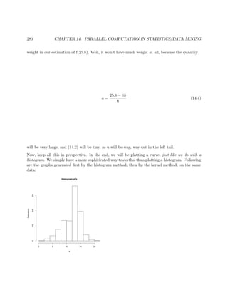
![282 CHAPTER 14. PARALLEL COMPUTATION IN STATISTICS/DATA MINING
14.2.2 Histogram Computation for Images
In image processing, histograms are used to find tallies of how many pixels there are of each
intensity. (Note that there is thus no interval width issue, as there is a separate “interval” value
for each possible intensity level.) The serial pseudocode is:
for i = 1,...,numintenslevels:
count = 0
for row = 1,...,numrows:
for col = 1,...,numcols:
if image[row][col] == i: count++
hist[i] = count
On the surface, this is certainly an “embarrassingly parallel” problem. In OpenMP, for instance,
we might have each thread handle a block of rows of the image, i.e. parallelize the for row loop.
In CUDA, we might have each thread handle an individual pixel, thus parallelizing the nested for
row/col loops.
However, to make this go fast is a challenge, say in CUDA, due to issues of what to store in shared
memory, when to swap it out, etc. A very nice account of fine-tuning this computation in CUDA
is given in Histogram Calculation in CUDA, by Victor Podlozhnyuk of NVIDIA, 2007, http://
developer.download.nvidia.com/compute/cuda/1_1/Website/projects/histogram256/doc/histogram.
pdf. The actual code is at http://developer.download.nvidia.com/compute/cuda/sdk/website/
Data-Parallel_Algorithms.html#histogram. A summary follows:
(Much of the research into understand Podlozhnyuk’s algorithm was done by UC Davis graduate
student Spencer Mathews.)
Podlozhnyuk’s overall plan is to have the threads compute subhistograms for various chunks of the
image, then merge the subhistograms to create the histogram for the entire data set. Each thread
will handle 1/k of the image’s pixels, where k is the total number of threads in the grid, i.e. across
all blocks.
In Podlozhnyuk’s first cut at the problem, he maintains a separate subhistogram for each thread. He
calls this version of the code histogram64. The name stems from the fact that only 64 intensity
levels are used, i.e. the more significant 6 bits of each pixel’s data byte. The reason for this
restriction will be discussed later.
Each thread will store its subhistogram as an array of bytes; the count of pixels that a thread finds
to have intensity i will be stored in the ith byte of this array. Considering the content of a byte as
an unsigned number, that means that each thread can process only 255 pixels.
the fact that the characteristic function of the sum of two independent random variables is equal to the product of
the characteristic functions of the two variables.](https://image.slidesharecdn.com/matloff-programmingonparallelmachines-2013-150626072019-lva1-app6892/85/Matloff-programming-on-parallel_machines-2013-302-320.jpg)
![284 CHAPTER 14. PARALLEL COMPUTATION IN STATISTICS/DATA MINING
q
q
q
qq
q
q
q
qq
q
q
q
q
q
q
q
q
q
q
q
q
qq
q
q
q
q
q
q
q
q
q
q
q
q q
q
q
q
q
q
q
q
q
q
q
q
q
q
q
q
q
q
q
q
q
q
q
q
q
q
q
q
q
q
q
q
q
q
q
q
q
q
q
q
q
q
q
q
q
q
q
q
q
q
q
q
q
q
q
q
q
q
q
q
q
q
q
q
q
q
qq
q
q
q
q
q
q
q
q
q
q
q
q
q
q
q
q
q
q
q
q
q
q
q
q
q
q
q
qq
q
q
q
q
q
q
q
q
q
q
q
q
q
q
q
q
q
q
q
q
q
q
q
q
q
q
q
q
q q
q
q
q
q
q
q
q
q
q
q
q
q
q
q
q
q
q
q
q
q
q
q
q
q
q
q
q
q
q
q
q
q
q
q
q
q
q
q
q
q
q
q
q
q
q
q
q
q
q
q
q
q
q
q
q
q
q
q
q
q
q
q
q
q q
q
q
q
q q
q
q
q
q
q
q
q
q
q
q
q
q
q
qq
q
q
q
q
q
q
q
q
q
q
q
q
q
q
q
q
q
q
q
q
q
q
q
q
qq
q
q
q
q
q
q
q
qq
q
q
q
q
q
q
q
q
q
q
q
q
q
q
q
q
q
q
q
q
q
q
q
q
q
q
q
qq
q
q
q
q
q
q
q
q
q q
q
q
q
q
q
qq
q
q
q q
q
q
q
q
q
q
q
q
q
q
qq
q
q
q
q
q
q
q
q
q
q
q
q
q
q
q q
q
q q
q
q
q
q
q
q
q
q
q
q
q
0 5 10 15 20
0510
xy[,1]
xy[,2]
It looks like there may be two or three groups here. What clustering algorithms do is to form
groups, both their number and their membership, i.e. which data points belong to which groups.
(Note carefully that there is no “correct” answer here. This is merely an exploratory data analysis
tool.)
Clustering is used is many diverse fields. For instance, it is used in image processing for segmentation
and edge detection.
Here we have to two variables, say people’s heights and weights. In general we have many variables,
say p of them, so whatever clustering we find will be in p-dimensional space. No, we can’t picture
it very easily of p is larger than (or even equal to) 3, but we can at least identify membership, i.e.
John and Mary are in group 1, Jenny is in group 2, etc. We may derive some insight from this.
There are many, many types of clustering algorithms. Here we will discuss the famous k-means
algorithm, developed by Prof. Jim MacQueen of the UCLA business school.
The method couldn’t be simpler. Choose k, the number of groups you want to form, and then run
this:
1 # form initial groups from the first k data points (or choose randomly)
2 for i = 1,...,k:
3 group[i] = (x[i],y[i])
4 center[i] = (x[i],y[i])
5 do:](https://image.slidesharecdn.com/matloff-programmingonparallelmachines-2013-150626072019-lva1-app6892/85/Matloff-programming-on-parallel_machines-2013-304-320.jpg)
![14.3. CLUSTERING 285
6 for j = 1,...,n:
7 find the closest center[i] to (x[j],y[j])
8 cl[j] = the i you got in the previous line
9 for i = 1,...,k:
10 group[i] = all (x[j],y[j]) such that cl[j] = i
11 center[i] = average of all (x,y) in group[i]
12 until group memberships do not change from one iteration to the next
Definitions of terms:
• Closest means in p-dimensional space, with the usual Euclidean distance: The distance from
(a1, ..., ap to (b1, ..., bp is
(b1 − a1)2 + ... + (bp − ap)2 (14.6)
Other distance definitions could be used too, of course.
• The center of a group is its centroid, which is a fancy name for taking the average value in
each component of the data points in the group. If p = 2, for example, the center consists
of the point whose X coordinate is the average X value among members of the group, and
whose Y coordinate is the average Y value in the group.
14.3.1 Example: k-Means Clustering in R
In terms of parallelization, again we have an embarrassingly parallel problem. Here’s snow code
for it:
1 # snow version of k−means c l u s t e r i n g problem
2
3 # returns distances from x to each vector in y ;
4 # here x i s a s i n g l e vector and y i s a bunch of them
5 #
6 # define distance between 2 points to be the sum of the absolute values
7 # of t h e i r componentwise d i f f e r e n c e s ; e . g . distance between ( 5 , 4 . 2 ) and
8 # ( 3 , 5 . 6 ) i s 2 + 1.4 = 3.4
9 dst <− function (x , y) {
10 tmpmat <− matrix ( abs (x−y ) , byrow=T, ncol=length (x )) # note r e c y c l i n g
11 rowSums(tmpmat)
12 }
13
14 # w i l l check t h i s worker ’ s mchunk matrix against currctrs , the current
15 # centers of the groups , returning a matrix ; row j of the matrix w i l l
16 # c o n s i s t of the vector sum of the points in mchunk c l o s e s t to j−th
17 # current center , and the count of such points
18 findnewgrps <− function ( c u r r c t r s ) {](https://image.slidesharecdn.com/matloff-programmingonparallelmachines-2013-150626072019-lva1-app6892/85/Matloff-programming-on-parallel_machines-2013-305-320.jpg)
![286 CHAPTER 14. PARALLEL COMPUTATION IN STATISTICS/DATA MINING
19 ngrps <− nrow ( c u r r c t r s )
20 spacedim <− ncol ( c u r r c t r s ) # what dimension space are we in ?
21 # set up the return matrix
22 sumcounts <− matrix ( rep (0 , ngrps ∗( spacedim +1)) ,nrow=ngrps )
23 f o r ( i in 1: nrow (mchunk )) {
24 dsts <− dst (mchunk [ i , ] , t ( c u r r c t r s ))
25 j <− which . min( dsts )
26 sumcounts [ j , ] <− sumcounts [ j , ] + c (mchunk [ i , ] , 1 )
27 }
28 sumcounts
29 }
30
31 parkm <− function ( cls ,m, niters , i n i t c e n t e r s ) {
32 n <− nrow (m)
33 spacedim <− ncol (m) # what dimension space are we in ?
34 # determine which worker gets which chunk of rows of m
35 options ( warn=−1)
36 ichunks <− s p l i t ( 1 : n , 1 : length ( c l s ))
37 options ( warn=0)
38 # form row chunks
39 mchunks <− lapply ( ichunks , function ( ichunk ) m[ ichunk , ] )
40 mcf <− function (mchunk) mchunk <<− mchunk
41 # send row chunks to workers ; each chunk w i l l be a global v a r i a b l e at
42 # the worker , named mchunk
43 i n v i s i b l e ( clusterApply ( cls , mchunks , mcf ))
44 # send dst () to workers
45 clusterExport ( cls ,” dst ”)
46 # s t a r t i t e r a t i o n s
47 centers <− i n i t c e n t e r s
48 f o r ( i in 1: n i t e r s ) {
49 sumcounts <− c l u s t e r C a l l ( cls , findnewgrps , centers )
50 tmp <− Reduce(”+” , sumcounts )
51 centers <− tmp [ , 1 : spacedim ] / tmp [ , spacedim +1]
52 # i f a group i s empty , let ’ s set i t s center to 0 s
53 centers [ i s . nan ( centers ) ] <− 0
54 }
55 centers
56 }
14.4 Principal Component Analysis (PCA)
Consider data consisting of (X,Y) pairs as we saw in Section 14.3. Suppose X and Y are highly
correlated with each other. Then for some constants c and d,
Y ≈ c + dX (14.7)](https://image.slidesharecdn.com/matloff-programmingonparallelmachines-2013-150626072019-lva1-app6892/85/Matloff-programming-on-parallel_machines-2013-306-320.jpg)
![A.3. ARRAY ISSUES 293
A.2.3 Performance Issues
Upon a cache miss, the hardware will need to read an entire block from memory, and if an eviction
is involved, an entire block will be written as well, assuming a write-back policy. (See the reference
at the beginning of this appendix.) All this is obviously slow.
The cache3 is quite small relative to memory, so you might guess that cache misses are very frequent.
Actually, though, they aren’t, due to something called locality of reference. This term refers to
the fact that most programs tend to either access the same memory item repeatedly within short
time periods (temporal locality), and/or access items within the same block often during short
periods (spatial locality). Hit rates are typically well above 90%. Part of this depends on having
a good block replacement policy, which decides which block to evict (hopefully one that won’t
be needed again soon!).
A page fault is pretty catastrophic in performance terms. Remember, the disk speed is on a
mechanical scale, not an electronic one, so it will take quite a while for the OS to service a page
fault, much worse than for a cache miss. So the page replacement policy is even more important
as well.
On Unix-family machines, the time command not only tells how long your program ran, but also
how many page faults it caused. Note that since the OS runs every time a page fault occurs, it
can keep track of the number of faults. This is very different from a cache miss, which although
seems similar to a page fault in many ways, the key point is that a cache miss is handled solely in
hardware, so no program can count the number of misses.4
Note that in a VM system each memory access becomes two memory accesses—the page table read
and the memory access itself. This would kill performance, so there is a special cache just for the
page table, called the Translation Lookaside Buffer.
A.3 Array Issues
A.3.1 Storage
It is important to understand how compilers store arrays in memory, an overview of which will now
be presented.
Consider the array declaration
int y [ 1 0 0 ] ;
3
Or caches, plural, as there are often multiple levels of caches in today’s machines.
4
Note by the way that cache misses, though harmful to program speed, aren’t as catastrophic as page faults, as
the disk is not involved.](https://image.slidesharecdn.com/matloff-programmingonparallelmachines-2013-150626072019-lva1-app6892/85/Matloff-programming-on-parallel_machines-2013-313-320.jpg)
![294 APPENDIX A. MISCELLANEOUS SYSTEMS ISSUES
The compiler will store this in 100 consecutive words of memory. You may recall that in C/C++,
an expression consisting of an array name, no subscript, is a pointer to the array. Well, more
specifically, it is the address of the first element of the array.
An array element, say y[8] actually means the same as the C/C++ pointer expression y+8, which
in turn means “the word 8 ints past the beginning of y.”
Two-dimensional arrays, say
int z [ 3 ] [ 1 0 ] ;
exist only in our imagination. They are actually treated as one-dimensional arrays, in the above
case consisting of 3 × 10 = 30 elements. C/C++ arranges this in row-major order, meaning that
all of row 0 comes first, then all of row 1 and so on. So for instance z [2][5] is stored in element
10 + 10 + 5 of z, and we could for example set that element to 8 with the code
z [ 2 5 ] = 8;
or
∗( z+25) = 8;
Note that if we have a c-column two-dimensional array, element (i,j) is stored in the word i×c+j of
the array. You’ll see this fact used a lot in this book, and in general in code written in the parallel
processing community.
A.3.2 Subarrays
The considerations in the last section can be used to access subarrays. For example, here is code
to find the sum of a float array of length k:
1 f l o a t sum( f l o a t x , int k)
2 { f l o a t s = 0 . 0 ; int i ;
3 f o r ( i = 0; i < k ; i++) s += x [ i ] ;
4 return s ;
5 }
Quite ordinary, but suppose we wish to find the sum in row 2 of the two-dimensional array z above.
We could do this as sum(z+20,10).
A.3.3 Memory Allocation
Very often one needs to set up an array whose size is not known at compile time. You are probably
accustomed to doing this via malloc() or new. However, in large parallel programs, this approach
may be quite slow.](https://image.slidesharecdn.com/matloff-programmingonparallelmachines-2013-150626072019-lva1-app6892/85/Matloff-programming-on-parallel_machines-2013-314-320.jpg)


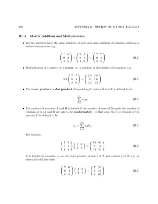

![Appendix C
R Quick Start
Here we present a quick introduction to the R data/statistical programming language. Further
learning resources are listed at http://heather.cs.ucdavis.edu/~/matloff/r.html.
R syntax is similar to that of C. It is object-oriented (in the sense of encapsulation, polymorphism
and everything being an object) and is a functional language (i.e. almost no side effects, every
action is a function call, etc.).
C.1 Correspondences
aspect C/C++ R
assignment = <- (or =)
array terminology array vector, matrix, array
subscripts start at 0 start at 1
array notation m[2][3] m[2,3]
2-D array storage row-major order column-major order
mixed container struct, members accessed by . list, members acessed by $ or [[ ]]
return mechanism return return() or last value computed
primitive types int, float, double, char, bool integer, float, double, character, logical
logical values true, false TRUE, FALSE (abbreviated T, F)
mechanism for combining modules include, link library()
run method batch interactive, batch
303](https://image.slidesharecdn.com/matloff-programmingonparallelmachines-2013-150626072019-lva1-app6892/85/Matloff-programming-on-parallel_machines-2013-323-320.jpg)
![304 APPENDIX C. R QUICK START
C.2 Starting R
To invoke R, just type “R” into a terminal window. On a Windows machine, you probably have
an R icon to click.
If you prefer to run from an IDE, you may wish to consider ESS for Emacs, StatET for Eclipse or
RStudio, all open source. ESS is the favorite among the “hard core coder” types, while the colorful,
easy-to-use, RStudio is a big general crowd pleaser. If you are already an Eclipse user, StatET will
be just what you need.
R is normally run in interactive mode, with > as the prompt. Among other things, that makes it
easy to try little experiments to learn from; remember my slogan, “When in doubt, try it out!”
C.3 First Sample Programming Session
Below is a commented R session, to introduce the concepts. I had a text editor open in another
window, constantly changing my code, then loading it via R’s source() command. The original
contents of the file odd.R were:
1 oddcount <− function (x) {
2 k <− 0 # assign 0 to k
3 f o r (n in x) {
4 i f (n %% 2 == 1) k <− k+1 # %% i s the modulo operator
5 }
6 return (k)
7 }
By the way, we could have written that last statement as simply
1 k
because the last computed value of an R function is returned automatically.
The R session is shown below. You may wish to type it yourself as you go along, trying little
experiments of your own along the way.1
1 > source (” odd .R”) # load code from the given f i l e
2 > l s () # what objects do we have?
3 [ 1 ] ”oddcount”
4 > # what kind of object i s oddcount ( well , we already know)?
5 > c l a s s ( oddcount )
6 [ 1 ] ” function ”
7 > # while in i n t e r a c t i v e mode , and not i n s i d e a function , can print
1
The source code for this file is at http://heather.cs.ucdavis.edu/~matloff/MiscPLN/R5MinIntro.tex. You
can download the file, and copy/paste the text from there.](https://image.slidesharecdn.com/matloff-programmingonparallelmachines-2013-150626072019-lva1-app6892/85/Matloff-programming-on-parallel_machines-2013-324-320.jpg)
![C.3. FIRST SAMPLE PROGRAMMING SESSION 305
8 > # any object by typing i t s name ; otherwise use print ( ) , e . g . print (x+y)
9 > oddcount # a function i s an object , so can print i t
10 function (x) {
11 k <− 0 # assign 0 to k
12 f o r (n in x) {
13 i f (n %% 2 == 1) k <− k+1 # %% i s the modulo operator
14 }
15 return (k)
16 }
17
18 > # let ’ s t e s t oddcount ( ) , but look at some p r o p e r t i e s of vectors f i r s t
19 > y <− c (5 ,12 ,13 ,8 ,88) # c () i s the concatenate function
20 > y
21 [ 1 ] 5 12 13 8 88
22 > y [ 2 ] # R s u b s c r i p t s begin at 1 , not 0
23 [ 1 ] 12
24 > y [ 2 : 4 ] # extract elements 2 , 3 and 4 of y
25 [ 1 ] 12 13 8
26 > y [ c ( 1 , 3 : 5 ) ] # elements 1 , 3 , 4 and 5
27 [ 1 ] 5 13 8 88
28 > oddcount (y) # should report 2 odd numbers
29 [ 1 ] 2
30
31 > # change code ( in the other window) to v e c t o r i z e the count operation ,
32 > # f o r much f a s t e r execution
33 > source (” odd .R”)
34 > oddcount
35 function (x) {
36 x1 <− (x %% 2 == 1) # x1 now a vector of TRUEs and FALSEs
37 x2 <− x [ x1 ] # x2 now has the elements of x that were TRUE in x1
38 return ( length ( x2 ))
39 }
40
41 > # try i t on subset of y , elements 2 through 3
42 > oddcount (y [ 2 : 3 ] )
43 [ 1 ] 1
44 > # try i t on subset of y , elements 2 , 4 and 5
45 > oddcount (y [ c ( 2 , 4 , 5 ) ] )
46 [ 1 ] 0
47
48 > # further compactify the code
49 > source (” odd .R”)
50 > oddcount
51 function (x) {
52 length (x [ x %% 2 == 1 ] ) # l a s t value computed i s auto returned
53 }
54 > oddcount (y) # t e s t i t
55 [ 1 ] 2
56
57 # and even more compactification , making use of the f a c t that TRUE and](https://image.slidesharecdn.com/matloff-programmingonparallelmachines-2013-150626072019-lva1-app6892/85/Matloff-programming-on-parallel_machines-2013-325-320.jpg)
![306 APPENDIX C. R QUICK START
58 # FALSE are treated as 1 and 0
59 > oddcount <− function (x) sum(x %% 2 == 1)
60 # make sure you understand the steps that that involves : x i s a vector ,
61 # and thus x %% 2 i s a new vector , the r e s u l t of applying the mod 2
62 # operation to every element of x ; then x %% 2 == 1 a p p l i e s the == 1
63 # operation to each element of that result , y i e l d i n g a new vector of TRUE
64 # and FALSE values ; sum() then adds them ( as 1 s and 0 s )
65
66 # we can also determine which elements are odd
67 > which (y %% 2 == 1)
68 [ 1 ] 1 3
69
70 > # now have ftn return odd count AND the odd numbers themselves , using
71 > # the R l i s t type
72 > source (” odd .R”)
73 > oddcount
74 function (x) {
75 x1 <− x [ x %% 2 == 1]
76 return ( l i s t ( odds=x1 , numodds=length ( x1 ) ) )
77 }
78 > # R’ s l i s t type can contain any type ; components delineated by $
79 > oddcount (y)
80 $odds
81 [ 1 ] 5 13
82
83 $numodds
84 [ 1 ] 2
85
86 > ocy <− oddcount (y) # save the output in ocy , which w i l l be a l i s t
87 > ocy
88 $odds
89 [ 1 ] 5 13
90
91 $numodds
92 [ 1 ] 2
93
94 > ocy$odds
95 [ 1 ] 5 13
96 > ocy [ [ 1 ] ] # can get l i s t elements using [ [ ] ] instead of $
97 [ 1 ] 5 13
98 > ocy [ [ 2 ] ]
99 [ 1 ] 2
Note that the function of the R function function() is to produce functions! Thus assignment is
used. For example, here is what odd.R looked like at the end of the above session:
1 oddcount <− function (x) {
2 x1 <− x [ x %% 2 == 1]
3 return ( l i s t ( odds=x1 , numodds=length ( x1 ) ) )
4 }](https://image.slidesharecdn.com/matloff-programmingonparallelmachines-2013-150626072019-lva1-app6892/85/Matloff-programming-on-parallel_machines-2013-326-320.jpg)
![C.4. SECOND SAMPLE PROGRAMMING SESSION 307
We created some code, and then used function() to create a function object, which we assigned
to oddcount.
Note that we eventually vectorized our function oddcount(). This means taking advantage of
the vector-based, functional language nature of R, exploiting R’s built-in functions instead of loops.
This changes the venue from interpreted R to C level, with a potentially large increase in speed.
For example:
1 > x <− r u n i f (1000000) # 1000000 random numbers from the i n t e r v a l (0 ,1)
2 > system . time (sum(x ))
3 user system elapsed
4 0.008 0.000 0.006
5 > system . time ({ s <− 0; f o r ( i in 1:1000000) s <− s + x [ i ] } )
6 user system elapsed
7 2.776 0.004 2.859
C.4 Second Sample Programming Session
A matrix is a special case of a vector, with added class attributes, the numbers of rows and columns.
1 > # ”rowbind () function combines rows of matrices ; there ’ s a cbind () too
2 > m1 <− rbind ( 1 : 2 , c (5 ,8))
3 > m1
4 [ , 1 ] [ , 2 ]
5 [ 1 , ] 1 2
6 [ 2 , ] 5 8
7 > rbind (m1, c (6 , −1))
8 [ , 1 ] [ , 2 ]
9 [ 1 , ] 1 2
10 [ 2 , ] 5 8
11 [ 3 , ] 6 −1
12
13 > # form matrix from 1 ,2 ,3 ,4 ,5 ,6 , in 2 rows ; R uses column−major storage
14 > m2 <− matrix ( 1 : 6 , nrow=2)
15 > m2
16 [ , 1 ] [ , 2 ] [ , 3 ]
17 [ 1 , ] 1 3 5
18 [ 2 , ] 2 4 6
19 > ncol (m2)
20 [ 1 ] 3
21 > nrow (m2)
22 [ 1 ] 2
23 > m2[ 2 , 3 ] # extract element in row 2 , col 3
24 [ 1 ] 6
25 # get submatrix of m2, c o l s 2 and 3 , any row
26 > m3 <− m2[ , 2 : 3 ]
27 > m3](https://image.slidesharecdn.com/matloff-programmingonparallelmachines-2013-150626072019-lva1-app6892/85/Matloff-programming-on-parallel_machines-2013-327-320.jpg)
![308 APPENDIX C. R QUICK START
28 [ , 1 ] [ , 2 ]
29 [ 1 , ] 3 5
30 [ 2 , ] 4 6
31
32 > m1 ∗ m3 # elementwise m u l t i p l i c a t i o n
33 [ , 1 ] [ , 2 ]
34 [ 1 , ] 3 10
35 [ 2 , ] 20 48
36 > 2.5 ∗ m3 # s c a l a r m u l t i p l i c a t i o n ( but see below )
37 [ , 1 ] [ , 2 ]
38 [ 1 , ] 7.5 12.5
39 [ 2 , ] 10.0 15.0
40 > m1 %∗% m3 # l i n e a r algebra matrix m u l t i p l i c a t i o n
41 [ , 1 ] [ , 2 ]
42 [ 1 , ] 11 17
43 [ 2 , ] 47 73
44
45 > # matrices are s p e c i a l cases of vectors , so can t r e a t them as vectors
46 > sum(m1)
47 [ 1 ] 16
48 > i f e l s e (m2 %%3 == 1 ,0 ,m2) # ( see below )
49 [ , 1 ] [ , 2 ] [ , 3 ]
50 [ 1 , ] 0 3 5
51 [ 2 , ] 2 0 6
The “scalar multiplication” above is not quite what you may think, even though the result may
be. Here’s why:
In R, scalars don’t really exist; they are just one-element vectors. However, R usually uses recy-
cling, i.e. replication, to make vector sizes match. In the example above in which we evaluated
the express 2.5 * m3, the number 2.5 was recycled to the matrix
2.5 2.5
2.5 2.5
(C.1)
in order to conform with m3 for (elementwise) multiplication.
The ifelse() function is another example of vectorization. Its call has the form
i f e l s e ( boolean vectorexpression1 , vectorexpression2 , vectorexpression3 )
All three vector expressions must be the same length, though R will lengthen some via recycling.
The action will be to return a vector of the same length (and if matrices are involved, then the
result also has the same shape). Each element of the result will be set to its corresponding element
in vectorexpression2 or vectorexpression3, depending on whether the corresponding element
in vectorexpression1 is TRUE or FALSE.](https://image.slidesharecdn.com/matloff-programmingonparallelmachines-2013-150626072019-lva1-app6892/85/Matloff-programming-on-parallel_machines-2013-328-320.jpg)
![C.5. THIRD SAMPLE PROGRAMMING SESSION 309
In our example above,
> i f e l s e (m2 %%3 == 1 ,0 ,m2) # ( see below )
the expression m2 %%3 == 1 evaluated to the boolean matrix
T F F
F T F
(C.2)
(TRUE and FALSE may be abbreviated to T and F.)
The 0 was recycled to the matrix
0 0 0
0 0 0
(C.3)
while vectorexpression3, m2, evaluated to itself.
C.5 Third Sample Programming Session
This time, we focus on vectors and matrices.
> m <− rbind ( 1 : 3 , c (5 ,12 ,13)) # ”row bind ,” combine rows
> m
[ , 1 ] [ , 2 ] [ , 3 ]
[ 1 , ] 1 2 3
[ 2 , ] 5 12 13
> t (m) # transpose
[ , 1 ] [ , 2 ]
[ 1 , ] 1 5
[ 2 , ] 2 12
[ 3 , ] 3 13
> ma <− m[ , 1 : 2 ]
> ma
[ , 1 ] [ , 2 ]
[ 1 , ] 1 2
[ 2 , ] 5 12
> rep (1 ,2) # ” repeat ,” make multiple copies
[ 1 ] 1 1
> ma %∗% rep (1 ,2) # matrix multiply
[ , 1 ]
[ 1 , ] 3
[ 2 , ] 17
> solve (ma, c (3 ,17)) # solve l i n e a r system
[ 1 ] 1 1](https://image.slidesharecdn.com/matloff-programmingonparallelmachines-2013-150626072019-lva1-app6892/85/Matloff-programming-on-parallel_machines-2013-329-320.jpg)
![310 APPENDIX C. R QUICK START
> solve (ma) # matrix inverse
[ , 1 ] [ , 2 ]
[ 1 , ] 6.0 −1.0
[ 2 , ] −2.5 0.5
C.6 The R List Type
The R list type is, after vectors, the most important R construct. A list is like a vector, except
that the components are generally of mixed types.
C.6.1 The Basics
Here is example usage:
> g <− l i s t (x = 4:6 , s = ”abc ”)
> g
$x
[ 1 ] 4 5 6
$s
[ 1 ] ”abc”
> g$x # can r e f e r e n c e by component name
[ 1 ] 4 5 6
> g$s
[ 1 ] ”abc”
> g [ [ 1 ] ] # can r e f e r e n c e by index , but note double brackets
[ 1 ] 4 5 6
> g [ [ 2 ] ]
[ 1 ] ”abc”
> f o r ( i in 1: length ( g )) print ( g [ [ i ] ] )
[ 1 ] 4 5 6
[ 1 ] ”abc”
C.6.2 The Reduce() Function
One often needs to combine elements of a list in some way. One approach to this is to use Reduce():
> x <− l i s t ( 4 : 6 , c (1 ,6 ,8))
> x
[ [ 1 ] ]
[ 1 ] 4 5 6](https://image.slidesharecdn.com/matloff-programmingonparallelmachines-2013-150626072019-lva1-app6892/85/Matloff-programming-on-parallel_machines-2013-330-320.jpg)
![C.6. THE R LIST TYPE 311
[ [ 2 ] ]
[ 1 ] 1 6 8
> sum(x)
Error in sum(x) : i n v a l i d ’ type ’ ( l i s t ) of argument
> Reduce (sum , x)
[ 1 ] 30
Here Reduce() cumulatively applied R’s sum() to x. Of course, you can use it with functions you
write yourself too.
Continuing the above example:
> Reduce ( c , x)
[ 1 ] 4 5 6 1 6 8
C.6.3 S3 Classes
R is an object-oriented (and functional) language. It features two types of classes, S3 and S4. I’ll
introduce S3 here.
An S3 object is simply a list, with a class name added as an attribute:
> j <− l i s t (name=”Joe ” , salary =55000, union=T)
> c l a s s ( j ) <− ”employee”
> m <− l i s t (name=”Joe ” , salary =55000, union=F)
> c l a s s (m) <− ”employee”
So now we have two objects of a class we’ve chosen to name ”employee”. Note the quotation
marks.
We can write class generic functions:
> print . employee <− function ( wrkr ) {
+ cat ( wrkr$name ,” n”)
+ cat (” salary ” , wrkr$salary ,” n”)
+ cat (” union member” , wrkr$union ,” n”)
+ }
> print ( j )
Joe
salary 55000
union member TRUE
> j
Joe
salary 55000
union member TRUE](https://image.slidesharecdn.com/matloff-programmingonparallelmachines-2013-150626072019-lva1-app6892/85/Matloff-programming-on-parallel_machines-2013-331-320.jpg)
![312 APPENDIX C. R QUICK START
What just happened? Well, print() in R is a generic function, meaning that it is just a placeholder
for a function specific to a given class. When we printed j above, the R interpreter searched for a
function print.employee(), which we had indeed created, and that is what was executed. Lacking
this, R would have used the print function for R lists, as before:
> rm( print . employee ) # remove the function , to see what happens with print
> j
$name
[ 1 ] ”Joe”
$salary
[ 1 ] 55000
$union
[ 1 ] TRUE
att r ( ,” c l a s s ”)
[ 1 ] ”employee”
C.6.4 Handy Utilities
R functions written by others, e.g. in base R or in the CRAN repository for user-contributed code,
often return values which are class objects. It is common, for instance, to have lists within lists. In
many cases these objects are quite intricate, and not thoroughly documented. In order to explore
the contents of an object—even one you write yourself—here are some handy utilities:
• names(): Returns the names of a list.
• str(): Shows the first few elements of each component.
• summary(): General function. The author of a class x can write a version specific to x,
i.e. summary.x(), to print out the important parts; otherwise the default will print some
bare-bones information.
For example:
> z <− l i s t ( a = r u n i f (50) , b = l i s t (u=sample (1:100 ,25) , v=”blue sky ”))
> z
$a
[ 1 ] 0.301676229 0.679918518 0.208713522 0.510032893 0.405027042
0.412388038
[ 7 ] 0.900498062 0.119936222 0.154996457 0.251126218 0.928304164
0.979945937
[ 1 3 ] 0.902377363 0.941813898 0.027964137 0.992137908 0.207571134
0.049504986](https://image.slidesharecdn.com/matloff-programmingonparallelmachines-2013-150626072019-lva1-app6892/85/Matloff-programming-on-parallel_machines-2013-332-320.jpg)
![C.7. GRAPHICS 313
[ 1 9 ] 0.092011899 0.564024424 0.247162004 0.730086786 0.530251779
0.562163986
[ 2 5 ] 0.360718988 0.392522242 0.830468427 0.883086752 0.009853107
0.148819125
[ 3 1 ] 0.381143870 0.027740959 0.173798926 0.338813042 0.371025885
0.417984331
[ 3 7 ] 0.777219084 0.588650413 0.916212011 0.181104510 0.377617399
0.856198893
[ 4 3 ] 0.629269146 0.921698394 0.878412398 0.771662408 0.595483477
0.940457376
[ 4 9 ] 0.228829858 0.700500359
$b
$b$u
[ 1 ] 33 67 32 76 29 3 42 54 97 41 57 87 36 92 81 31 78 12 85 73 26 44
86 40 43
$b$v
[ 1 ] ” blue sky”
> names ( z )
[ 1 ] ”a” ”b”
> s t r ( z )
List of 2
$ a : num [ 1 : 5 0 ] 0.302 0.68 0.209 0.51 0.405 . . .
$ b : List of 2
. . $ u : int [ 1 : 2 5 ] 33 67 32 76 29 3 42 54 97 41 . . .
. . $ v : chr ” blue sky”
> names ( z$b )
[ 1 ] ”u” ”v”
> summary( z )
Length Class Mode
a 50 −none− numeric
b 2 −none− l i s t
C.7 Graphics
R excels at graphics, offering a rich set of capabilities, from beginning to advanced. In addition to
the functions in base R, extensive graphics packages are available, such as lattice and ggplot2.
One point of confusion for beginniners involves saving an R graph that is currently displayed on
the screen to a file. Here is a function for this, which I include in my R startup file, .Rprofile, in
my home directory:
p r 2 f i l e
function ( filename )
{
origdev <− dev . cur ()](https://image.slidesharecdn.com/matloff-programmingonparallelmachines-2013-150626072019-lva1-app6892/85/Matloff-programming-on-parallel_machines-2013-333-320.jpg)
![314 APPENDIX C. R QUICK START
parts <− s t r s p l i t ( filename , ”.” , f i x e d = TRUE)
nparts <− length ( parts [ [ 1 ] ] )
s u f f <− parts [ [ 1 ] ] [ nparts ]
i f ( s u f f == ”pdf ”) {
pdf ( filename )
}
e l s e i f ( s u f f == ”png ”) {
png ( filename )
}
e l s e jpeg ( filename )
devnum <− dev . cur ()
dev . set ( origdev )
dev . copy ( which = devnum)
dev . set (devnum)
dev . o f f ()
dev . set ( origdev )
}
The code, which I won’t go into here, mostly involves manipulation of various R graphics devices.
I’ve set it up so that you can save to a file of type either PDF, PNG or JPEG, implied by the file
name you give.
C.8 Other Sources for Learning R
There are tons of resources for R on the Web. You may wish to start with the links at http:
//heather.cs.ucdavis.edu/~matloff/r.html.
C.9 Online Help
R’s help() function, which can be invoked also with a question mark, gives short descriptions of
the R functions. For example, typing
> ?rep
will give you a description of R’s rep() function.
An especially nice feature of R is its example() function, which gives nice examples of whatever
function you wish to query. For instance, typing
> example ( wireframe ( ) )
will show examples—R code and resulting pictures—of wireframe(), one of R’s 3-dimensional
graphics functions.](https://image.slidesharecdn.com/matloff-programmingonparallelmachines-2013-150626072019-lva1-app6892/85/Matloff-programming-on-parallel_machines-2013-334-320.jpg)
![C.10. DEBUGGING IN R 315
C.10 Debugging in R
The internal debugging tool in R, debug(), is usable but rather primitive. Here are some alterna-
tives:
• The RStudio IDE has a built-in debugging tool.
• The StatET IDE for R on Eclipse has a nice debugging tool. Works on all major platforms,
but can be tricky to install.
• My own debugging tool, debugR, is extensive and easy to install, but for the time being is lim-
ited to Linux, Mac and other Unix-family systems. See http://heather.cs.ucdavis.edu/debugR.html.
C.11 Complex Numbers
If you have need for complex numbers, R does handle them. Here is a sample of use of the main
functions of interest:
> za <− complex ( r e a l =2, imaginary =3.5)
> za
[ 1 ] 2+3.5 i
> zb <− complex ( r e a l =1, imaginary=−5)
> zb
[ 1 ] 1−5 i
> za ∗ zb
[ 1 ] 19.5 −6.5 i
> Re( za )
[ 1 ] 2
> Im( za )
[ 1 ] 3.5
> za ˆ2
[ 1 ] −8.25+14 i
> abs ( za )
[ 1 ] 4.031129
> exp ( complex ( r e a l =0, imaginary=pi /4))
[ 1 ] 0.7071068+0.7071068 i
> cos ( pi /4)
[ 1 ] 0.7071068
> sin ( pi /4)
[ 1 ] 0.7071068
Note that operations with complex-valued vectors and matrices work as usual; there are no special
complex functions.](https://image.slidesharecdn.com/matloff-programmingonparallelmachines-2013-150626072019-lva1-app6892/85/Matloff-programming-on-parallel_machines-2013-335-320.jpg)

This document provides a biography and overview of a textbook about programming on parallel machines by Norm Matloff. It discusses that the book focuses on practical parallel programming using platforms like OpenMP, CUDA and MPI. It is aimed at students who are reasonably proficient in programming and linear algebra. The book uses examples in C/C++ and R to illustrate fundamental parallelization principles.