Facility Layout
Layoutrefers to the configuration of departments, work centers,
and equipment, with particular emphasis on movement of work
(customers or materials) through the system.
Layout decisions are important for three basic reasons:
1. require substantial investments of money and effort;
2. involve long-term commitments, which makes mistakes difficult
to overcome; and
3. have a significant impact on the cost and efficiency of
operations
3.
Factors affecting Plant
Layout
1.Plant location and building
2. Nature of Product
3. Type of Industry
4. Plant Environment
5. Spatial Requirements
6. Repairs and Maintenance
7. Balance
8. Management Policy
9. Human Needs
10. Types of machinery and equipment
4.
Factors affecting Plant
Layout
The basic objective of layout design is to facilitate a smooth flow of
work, material, and information through the system. Supporting
objectives generally involve the following:
To facilitate attainment of product or service quality.
To use workers and space efficiently.
To avoid bottlenecks.
To minimize material handling costs.
To eliminate unnecessary movements of workers or materials.
To minimize production time or customer service time.
To design for safety.
5.
Plant Layout :Types
The production process normally determines the type of plant layout
to be applied to the facility:
• Fixed position plant layout
Product stays and resources move to it.
• Product oriented plant layout
Machinery and Materials are placed following the product
path
• Process oriented plant layout (Functional Layout).
Machinery is placed according to what they do and materials
go to them.
• Combined Layout
Combine aspects of both process and product layouts
6.
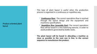
Product oriented plant
layout
This type of plant layout is useful when the production
process is organized in a continuous or repetitive way.
Continuous flow : The correct operations flow is reached
through the layout design and the equipment and
machinery specifications.
Repetitive flow (assembly line): The correct operations
flow will be based in a line balancing exercise, in order to
avoid problems generated by bottle necks.
The plant layout will be based in allocating a machine as
close as possible to the next one in line, in the correct
sequence to manufacture the product.
7.
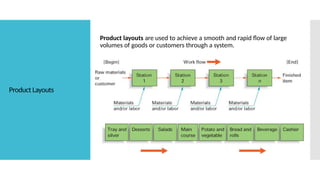
Product Layouts
Product layoutsare used to achieve a smooth and rapid flow of large
volumes of goods or customers through a system.
8.
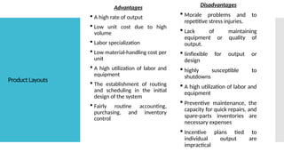
Product Layouts
Disadvantages
Moraleproblems and to
repetitive stress injuries.
Lack of maintaining
equipment or quality of
output.
Iinflexible for output or
design
highly susceptible to
shutdowns
A high utilization of labor and
equipment
Preventive maintenance, the
capacity for quick repairs, and
spare-parts inventories are
necessary expenses
Incentive plans tied to
individual output are
impractical
Advantages
A high rate of output
Low unit cost due to high
volume
Labor specialization
Low material-handling cost per
unit
A high utilization of labor and
equipment
The establishment of routing
and scheduling in the initial
design of the system
Fairly routine accounting,
purchasing, and inventory
control
9.
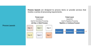
Process Layouts
Processlayouts are designed to process items or provide services that
involve a variety of processing requirements.
10.
Process oriented plant
layout(Functional
Layout)
This type of plant layout is useful when the production
process is organized in batches.
Personnel and equipment to perform the same function are
allocated in the same area.
The different items have to move from one area to another
one, according to the sequence of operations previously
established.
The variety of products to produce will lead to a diversity of
flows through the facility.
The variations in the production volumes from one period to
the next one (short periods of time) may lead to modifications
in the manufactured quantities as well as the types of
products to be produced.
11.
Process Layout
Advantages
Handlea variety of processing
requirements
Not vulnerable to equipment
failures
General-purpose equipment is
less costly and is easier and less
costly to maintain
Possible to use individual
incentive systems
Disadvantages
In-process inventory costs can be high
Routing and scheduling pose
continual challenges
Equipment utilization rates are low
Material handling is slow and
inefficient, and more costly per unit
Job complexities reduce the span of
supervision and result higher
supervisory costs
Special attention necessary for each
product or customer and low volumes
result in higher unit costs
Accounting, inventory control, and
purchasing are much more involved
12.
Fixed-Position Layouts
Infixed-position layouts, the item being worked on remains
stationary, and workers, materials, and equipment are moved
about as needed.
Fixed-position layouts are widely used in farming, firefighting, road
building, home building, remodeling and repair, and drilling for oil.
In each case, compelling reasons bring workers, materials, and
equipment to the “product’s” location instead of the other way
around.
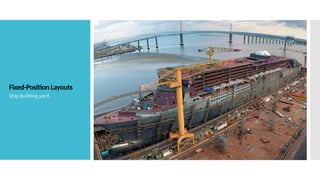
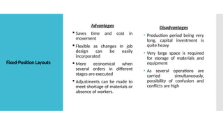
Fixed-Position Layouts
Advantages
Savestime and cost in
movement
Flexible as changes in job
design can be easily
incorporated
More economical when
several orders in different
stages are executed
Adjustments can be made to
meet shortage of materials or
absence of workers.
Disadvantages
• Production period being very
long, capital investment is
quite heavy
• Very large space is required
for storage of materials and
equipment
• As several operations are
carried simultaneously,
possibility of confusion and
conflicts are high
15.
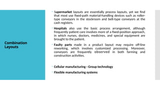
Combination
Layouts
Supermarket layoutsare essentially process layouts, yet we find
that most use fixed-path material-handling devices such as roller-
type conveyors in the stockroom and belt-type conveyors at the
cash registers.
Hospitals also use the basic process arrangement, although
frequently patient care involves more of a fixed-position approach,
in which nurses, doctors, medicines, and special equipment are
brought to the patient.
Faulty parts made in a product layout may require off-line
reworking, which involves customized processing. Moreover,
conveyors are frequently observed in both farming and
construction activities.
Cellular manufacturing - Group technology
Flexible manufacturing systems
16.
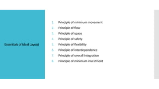
Essentials of IdealLayout
1. Principle of minimum movement
2. Principle of flow
3. Principle of space
4. Principle of safety
5. Principle of flexibility
6. Principle of interdependence
7. Principle of overall integration
8. Principle of minimum investment
17.
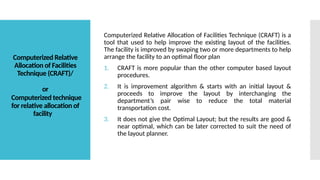
Computerized Relative
Allocation ofFacilities
Technique (CRAFT)/
or
Computerized technique
for relative allocation of
facility
Computerized Relative Allocation of Facilities Technique (CRAFT) is a
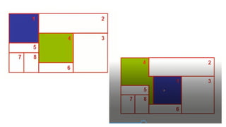
tool that used to help improve the existing layout of the facilities.
The facility is improved by swaping two or more departments to help
arrange the facility to an optimal floor plan
1. CRAFT is more popular than the other computer based layout
procedures.
2. It is improvement algorithm & starts with an initial layout &
proceeds to improve the layout by interchanging the
department’s pair wise to reduce the total material
transportation cost.
3. It does not give the Optimal Layout; but the results are good &
near optimal, which can be later corrected to suit the need of
the layout planner.
18.
Features of CRAFT
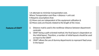
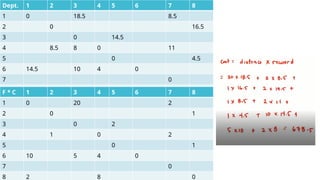
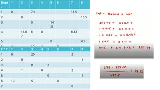
1.Itattempts to minimize transportation cost,
Where Transportation cost=flow × distance × unit cost
It Requires assumptions that:
(1) Move cost are independent of the equipment utilization &
(2) Move costs are linearly related to the length of the move.
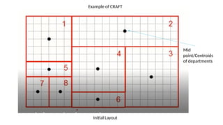
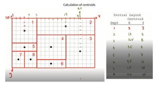
2. Distance matrix used is the rectilinear distance between department
centroids
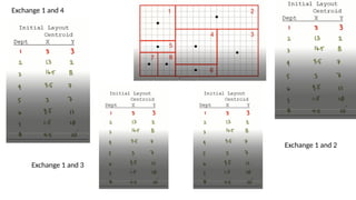
3. CRAFT being a path-oriented method, the final layout is dependent on
the initial layout. Therefore, a number of initial layouts should be used
as input to the CRAFT
4. CRAFT allows the use of dummy departments to represent fixed areas
in the layout
19.
Features of CRAFT
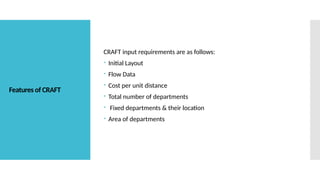
CRAFTinput requirements are as follows:
Initial Layout
Flow Data
Cost per unit distance
Total number of departments
Fixed departments & their location
Area of departments
20.
CRAFT
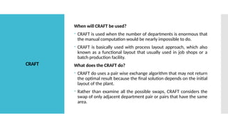
When will CRAFTbe used?
CRAFT is used when the number of departments is enormous that
the manual computation would be nearly impossible to do.
CRAFT is basically used with process layout approach, which also
known as a functional layout that usually used in job shops or a
batch production facility.
What does the CRAFT do?
CRAFT do uses a pair wise exchange algorithm that may not return
the optimal result because the final solution depends on the initial
layout of the plant.
Rather than examine all the possible swaps, CRAFT considers the
swap of only adjacent department pair or pairs that have the same
area.
21.
Steps of usingCRAFT
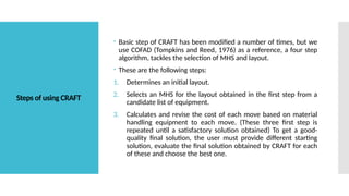
Basic step of CRAFT has been modified a number of times, but we
use COFAD (Tompkins and Reed, 1976) as a reference, a four step
algorithm, tackles the selection of MHS and layout.
These are the following steps:
1. Determines an initial layout.
2. Selects an MHS for the layout obtained in the first step from a
candidate list of equipment.
3. Calculates and revise the cost of each move based on material
handling equipment to each move. (These three first step is
repeated until a satisfactory solution obtained) To get a good-
quality final solution, the user must provide different starting
solution, evaluate the final solution obtained by CRAFT for each
of these and choose the best one.
22.
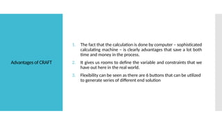
Advantages of CRAFT
1.The fact that the calculation is done by computer – sophisticated
calculating machine – is clearly advantages that save a lot both
time and money in the process.
2. It gives us rooms to define the variable and constraints that we
have out here in the real world.
3. Flexibility can be seen as there are 6 buttons that can be utilized
to generate series of different end solution
23.
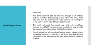
disadvantages of CRAFT
1.Inefficient
2. Jobs time occurred Jobs do not flow through in an orderly
fashion, therefore backtracking occurs often. Idle time, more
idle time may be experienced while workers are waiting for
more work to arrive from different departments.
3. The (not) end result. End result may need to be modified,
because once CRAFT has determined a solution it may need to
be managed to create a layout that fits in the plant.
4. Greedy algorithm. It is the algorithm that always takes the best
immediate solution. In contrary, a job shop that flow through
the system is not always constant and causes fluctuations in the
process.
Dept 1 23 4 5 6 7 8
1 0 18.5 8.5
2 0 16.5
3 0 14.5
4 8.5 8 0 11
5 0 4.5
6 14.5 10 4 0
7 0
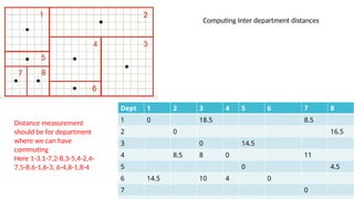
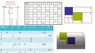
Computing Inter department distances
Distance measurement
should be for department
where we can have
commuting
Here 1-3,1-7,2-8,3-5,4-2,4-
7,5-8,6-1,6-3, 6-4,8-1,8-4
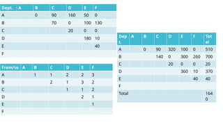
Problem 1
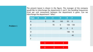
The presentlayout is shown in the figure. The manager of the company
would like to interchange the department C and F. the handling frequencies
(Cost per unit movement) between the department is given. Can we
interchange the department ? Why?
A
F
C E
B D
Dept. A B C D E F
A 0 90 160 50 0
B 70 0 100 130
C 20 0 0
D 180 10
E 40
F
33.
Solutions
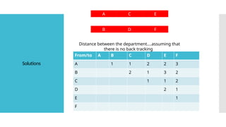
From/to A BC D E F
A 1 1 2 2 3
B 2 1 3 2
C 1 1 2
D 2 1
E 1
F
A
F
C E
B D
Distance between the department….assuming that
there is no back tracking
34.
Dept. A BC D E F
A 0 90 160 50 0
B 70 0 100 130
C 20 0 0
D 180 10
E 40
F
From/to A B C D E F
A 1 1 2 2 3
B 2 1 3 2
C 1 1 2
D 2 1
E 1
F
Dep
t.
A B C D E F Tot
al
A 0 90 320 100 0 510
B 140 0 300 260 700
C 20 0 0 20
D 360 10 370
E 40 40
F
Total 164
0
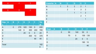
35.
A
C
F E
B D
From/toA B C D E F
A 1 3 2 2 1
B 2 1 3 2
C 1 1 2
D 2 1
E 1
F
Dept. A B C D E F
A 0 90 160 50 0
B 70 0 100 130
C 20 0 0
D 180 10
E 40
F
Dep
t.
A B C D E F Tot
al
A 0 270 320 100 0 690
B 140 0 300 260 700
C 20 0 0 20
D 360 10 370
E 40 40
F
Total 182
0
36.
Problem 2
The defensecontractor is evaluating its machine shops current process
layout. Figure shows the current process layout and the table shows the
current trip matrix for the facilities. Health and safety regulation demanded
fixed position of department E and F. Can we change the layout? If yes then
propose the new one with resuced cost
E
D
B F
A C
Dept. A B C D E F
A 8 3 9 5
B 3
C 8 9
D 3
E 3
F
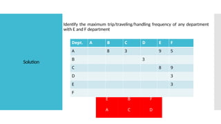
37.
Solution
Identify the maximumtrip/traveling/handling frequency of any department
with E and F department
E
D
B F
A C
Dept. A B C D E F
A 8 3 9 5
B 3
C 8 9
D 3
E 3
F
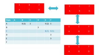
38.
E
D
C F
A B
E
D
BF
A C
E
D
C F
A B
E
D
C F
A B
Dept. A B C D E F
A 8 (3) 3 9 (2) 5
B 3
C 8 (1) 9 (1)
D 3
E 3
F
39.
E
D
B F
A C
E
D
CF
A B
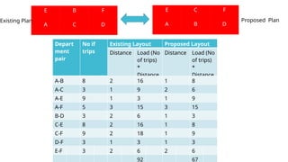
Existing Plan Proposed Plan
Depart
ment
pair
No if
trips
Existing Layout Proposed Layout
Distance Load (No
of trips)
*
Distance
Distance Load (No
of trips)
*
Distance
A-B 8 2 16 1 8
A-C 3 1 9 2 6
A-E 9 1 3 1 9
A-F 5 3 15 3 15
B-D 3 2 6 1 3
C-E 8 2 16 1 8
C-F 9 2 18 1 9
D-F 3 1 3 1 3
E-F 3 2 6 2 6
92 67
40.
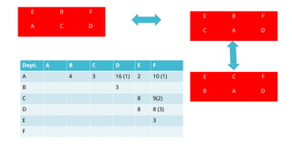
Problem 3
The defensecontractor is evaluating its machine shops current process
layout. Figure shows the current process layout and the table shows the
current trip matrix for the facilities. Health and safety regulation demanded
fixed position of department A. Can we change the layout? If yes then
propose the new one with reduced cost
E
D
B F
A C
Dept. A B C D E F
A 4 3 16 2 10
B 3
C 8 9
D 8 8
E 3
F
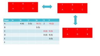
41.
Dept. A BC D E F
A 4 (4) 3 (5) 16 (1) 2 10 (2)
B 3 (5)
C 8 (3) 9 (3)
D 8 (4) 8 (4)
E 3 (5)
F
E
D
B F
A C
F
B
C E
A D
F
C
B E
A D
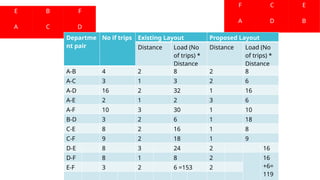
42.
F
B
C E
A D
E
D
BF
A C
Departme
nt pair
No if trips Existing Layout Proposed Layout
Distance Load (No
of trips) *
Distance
Distance Load (No
of trips) *
Distance
A-B 4 2 8 2 8
A-C 3 1 3 2 6
A-D 16 2 32 1 16
A-E 2 1 2 3 6
A-F 10 3 30 1 10
B-D 3 2 6 1 18
C-E 8 2 16 1 8
C-F 9 2 18 1 9
D-E 8 3 24 2 16
D-F 8 1 8 2 16
+6=
119
E-F 3 2 6 =153 2
43.
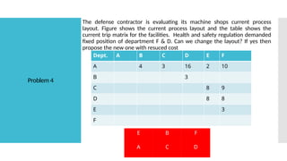
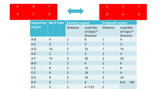
Problem 4
The defensecontractor is evaluating its machine shops current process
layout. Figure shows the current process layout and the table shows the
current trip matrix for the facilities. Health and safety regulation demanded
fixed position of department F & D. Can we change the layout? If yes then
propose the new one with resuced cost
E
D
B F
A C
Dept. A B C D E F
A 4 3 16 2 10
B 3
C 8 9
D 8 8
E 3
F
44.
E
D
C F
B A
Dept.A B C D E F
A 4 3 16 (1) 2 10 (1)
B 3
C 8 9(2)
D 8 8 (3)
E 3
F
E
D
B F
A C
E
D
B F
C A
45.
E
D
C F
B A
E
D
BF
A C
Departme
nt pair
No if trips Existing Layout Proposed Layout
Distance Load (No
of trips) *
Distance
Distance Load (No
of trips) *
Distance
A-B 4 2 8 1 4
A-C 3 1 3 1 3
A-D 16 2 32 1 16
A-E 2 1 2 2 4
A-F 10 3 30 2 20
B-D 3 2 6 2 6
C-E 8 2 16 1 8
C-F 9 2 18 1 9
D-E 8 3 24 3 24
D-F 8 1 8 1 8+6 108
E-F 3 2 6 =153 2
What is
MRP?
ComputerizedInventory Control
Production Planning System
Management Information System
Manufacturing Control System
48.
What is
MRP?
Thisis the most comprehensive approach to
manufacturing inventory and other dependents
which demand an efficient inventory management
system.
49.
What is MRP
do?
The MRP system determines item-by-item, what
is to be processed and when, as well as what is
to be manufactured when.
This is based on order priorities and available
capacities.
50.
When to use
MRP
Job Shop Production
Complex Products
Assemble-to-Order Environments
Discrete and Dependent Demand Items
51.
What can
MRP do?
Reduce Inventory Levels
Reduce Component Shortages
Improve Shipping Performance
Improve Customer Service
Improve Productivity
Simplified and Accurate Scheduling
Reduce Purchasing Cost
Improve Production Schedules
Reduce Manufacturing Cost
Reduce Lead Times
Less Scrap and Rework
Higher Production Quality
52.
What can
MRP do?
Improve Communication
Improve Plant Efficiency
Reduce Freight Cost
Reduction in Excess Inventory
Reduce Overtime
Improve Supply Schedules
Improve Calculation of Material Requirements
Improve Competitive Position
53.
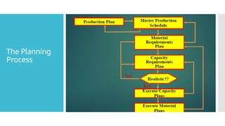
Three Basic
Steps ofMRP
Identifying Requirements
Running MRP – Creating the Suggestions
Firming the Suggestions
54.
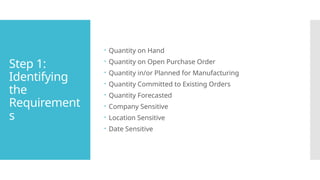
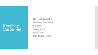
Step 1:
Identifying
the
Requirement
s
Quantityon Hand
Quantity on Open Purchase Order
Quantity in/or Planned for Manufacturing
Quantity Committed to Existing Orders
Quantity Forecasted
Company Sensitive
Location Sensitive
Date Sensitive
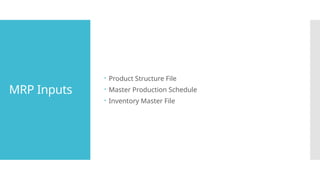
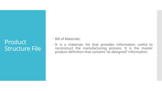
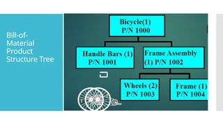
Product
Structure File
Billof Materials:
It is a materials list that provides information useful to
reconstruct the manufacturing process. It is the master
product definition that contains “as designed” information.
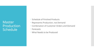
Master
Production
Schedule
Schedule ofFinished Products
Represents Production, not Demand
Combination of Customer Orders and Demand
Forecasts
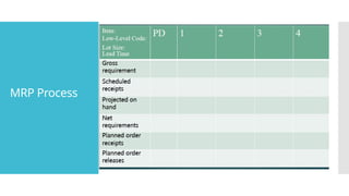
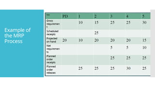
What Needs to be Produced
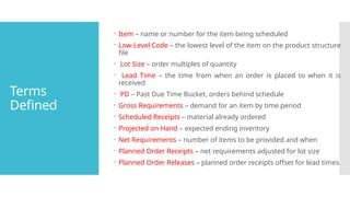
Terms
Defined
Item –name or number for the item being scheduled
Low-Level Code – the lowest level of the item on the product structure
file
Lot Size – order multiples of quantity
Lead Time – the time from when an order is placed to when it is
received
PD – Past Due Time Bucket, orders behind schedule
Gross Requirements – demand for an item by time period
Scheduled Receipts – material already ordered
Projected on Hand – expected ending inventory
Net Requirements – number of items to be provided and when
Planned Order Receipts – net requirements adjusted for lot size
Planned Order Releases – planned order receipts offset for lead times
Amul industryRajkot:- Mahindra & Walks wagon for shaft
manufacturing
2013:- 160 Rs, 95 rs……180 rs ………800 Cr …..850 Cr
On hand case, Operating revenue ……borrow from
market…reduce your profit …pay interest…..worth of
money money is keep on decreasing because the inflation
is increases
68.
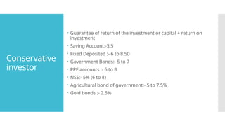
Conservative
investor
Guarantee ofreturn of the investment or capital + return on
investment
Saving Account:-3.5
Fixed Deposited :- 6 to 8.50
Government Bonds:- 5 to 7
PPF accounts :- 6 to 8
NSS:- 5% (6 to 8)
Agricultural bond of government:- 5 to 7.5%
Gold bonds :- 2.5%
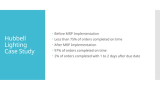
Hubbell
Lighting
Case Study
BeforeMRP Implementation
Less than 75% of orders completed on time
After MRP Implementation
97% of orders completed on time
2% of orders completed with 1 to 2 days after due date
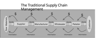
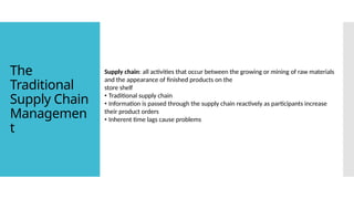
Supply chain: allactivities that occur between the growing or mining of raw materials
and the appearance of finished products on the
store shelf
• Traditional supply chain
• Information is passed through the supply chain reactively as participants increase
their product orders
• Inherent time lags cause problems
The
Traditional
Supply Chain
Managemen
t
77.
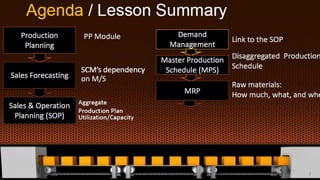
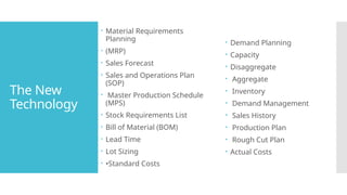
The New
Technology
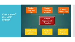
MaterialRequirements
Planning
(MRP)
Sales Forecast
Sales and Operations Plan
(SOP)
Master Production Schedule
(MPS)
Stock Requirements List
Bill of Material (BOM)
Lead Time
Lot Sizing
•Standard Costs
Demand Planning
Capacity
Disaggregate
Aggregate
Inventory
Demand Management
Sales History
Production Plan
Rough Cut Plan
Actual Costs
78.
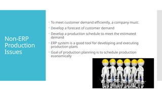
Non-ERP
Production
Issues
To meetcustomer demand efficiently, a company must:
Develop a forecast of customer demand
Develop a production schedule to meet the estimated
demand
ERP system is a good tool for developing and executing
production plans
Goal of production planning is to schedule production
economically
Communicatio
n problems
Marketingand Sales personnel do not share information
with Production personnel
Production personnel find it hard to deal with sudden
increases in demand might cause shortages or stock out
81.
Production
Problems
Inventory problems
Productionmanager lacks systematic method for:
Meeting anticipated sales demand
Adjusting production to reflect actual sales
Accounting and purchasing problems
The Production and Accounting Depts. must periodically
compare
standard costs (normal costs of manufacturing a product)
with actual costs (overhead and labor)and then adjust the
accounts
for the inevitable differences
82.
The
Production
Planning ERP
Process
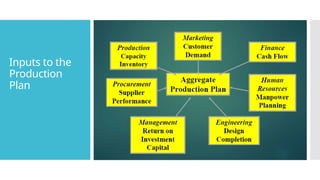
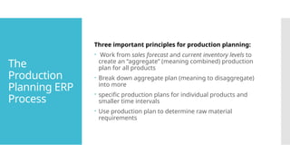
Three importantprinciples for production planning:
Work from sales forecast and current inventory levels to
create an “aggregate” (meaning combined) production
plan for all products
Break down aggregate plan (meaning to disaggregate)
into more
specific production plans for individual products and
smaller time intervals
Use production plan to determine raw material
requirements
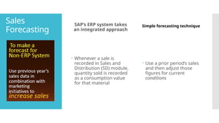
Sales
Forecasting
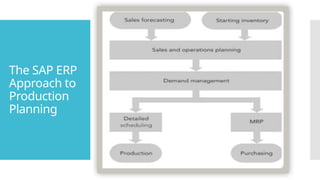
SAP’s ERP systemtakes
an integrated approach
Whenever a sale is
recorded in Sales and
Distribution (SD) module,
quantity sold is recorded
as a consumption value
for that material
Simple forecasting technique
Use a prior period’s sales
and then adjust those
figures for current
conditions
86.
Sales &
Operations
Planning
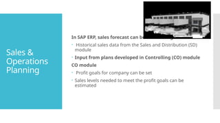
In SAPERP, sales forecast can be made using:
Historical sales data from the Sales and Distribution (SD)
module
Input from plans developed in Controlling (CO) module
CO module
Profit goals for company can be set
Sales levels needed to meet the profit goals can be
estimated
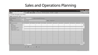
87.
Sales &
Operations
Planning
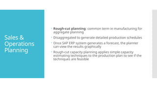
Rough-cutplanning: common term in manufacturing for
aggregate planning
Disaggregated to generate detailed production schedules
Once SAP ERP system generates a forecast, the planner
can view the results graphically
Rough-cut capacity planning applies simple capacity
estimating techniques to the production plan to see if the
techniques are feasible
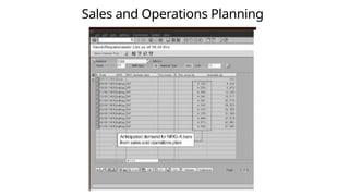
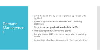
Demand
Managemen
t
Links thesales and operations planning process with
detailed
scheduling and materials requirements planning
processes
Output: master production schedule (MPS)
Production plan for all finished goods
For a business, MPS is an input to detailed scheduling,
which
determines what bars to make and when to make them
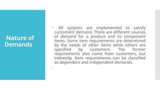
93.
Nature of
Demands
Allsystems are implemented to satisfy
customers’ demand. There are different sources
of demand for a product and its component
items. Some item requirements are determined
by the needs of other items while others are
specified by customers. The former
requirements also come from customers, but
indirectly. Item requirements can be classified
as dependent and independent demands.
94.
Independent
demand
Demand foran item that is unrelated to the
demand for other items. Demand for finished
goods, parts required for destructive testing,
and service part requirements are examples of
independent demand.
95.
MRP
Procedure
MPS procedureconsolidates the independent
demands of forecasts and customer orders to
determine the requirements of the end
products in each time bucket in the planning
horizon. After netting the on-hand and on-order
inventory, and offsetting the lead-time, the
production schedule of the end products, MPS,
is determined. In MPS procedure, the available-
to-promise (ATP) is also determined. MPS is then
fed into the MRP procedure to determine the
requirements of the lower level components
and raw materials.
96.
Dependent
demand
Demand thatis directly related to or derived
from the bill of material structure for other
items or end products. Such demands are
calculated and need not be forecasted.
A given inventory item may have both
dependent and independent demand at any
given time. For example, a part may
simultaneously be used as a component of an
assembly and also sold as a service part.
Production to meet dependent demand should
be scheduled so as to explicitly recognize its
linkage to production intended to meet
independent demand.
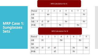
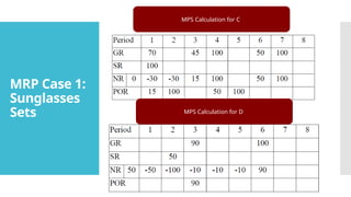
97.
MRP
Procedure
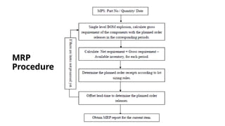
The grossrequirements of components are
determined by calculating the planned order
releases (POR) of the parents via single level BOM
explosion. The net requirements are calculated by
subtracting the on-hand inventory and scheduled
receipts (on-order) in each time bucket. After the
consideration of lot-size, the net requirements are
transformed into the planned order receipts.
Planned order receipts appear in every period. Lead-
time offsetting shifts the planned order receipts
backward and derives the POR which are the MRP
result of current item. The MRP procedure continues
to explode the POR to obtain the gross requirements
of its components. The MRP repeat the procedure
until the POR of all the items are determined. The
flow chart of the MRP procedure is described in
Figure
98.
MRP
Procedure
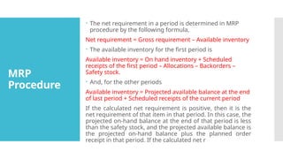
The netrequirement in a period is determined in MRP
procedure by the following formula,
Net requirement = Gross requirement – Available inventory
The available inventory for the first period is
Available inventory = On hand inventory + Scheduled
receipts of the first period – Allocations – Backorders –
Safety stock.
And, for the other periods
Available inventory = Projected available balance at the end
of last period + Scheduled receipts of the current period
If the calculated net requirement is positive, then it is the
net requirement of that item in that period. In this case, the
projected on-hand balance at the end of that period is less
than the safety stock, and the projected available balance is
the projected on-hand balance plus the planned order
receipt in that period. If the calculated net r
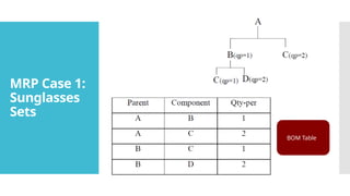
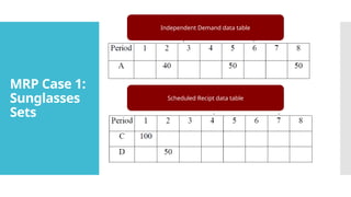
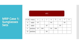
MRP Case 1:
Sunglasses
Sets
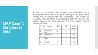
In the end product, two temples are assembled to a
single-piece lens to make a pair of sunglasses. Two spare
lenses are sold along with the sunglasses. They are put in
a plastic bag to form a sunglasses set. We ignore the
plastic bag in the end product. The item master file is
shown in Table
102.
MRP Case 1:
Sunglasses
Sets
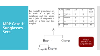
Product
Structurefor
Sunglasses Set
For example, a sunglasses set
is made of a pair of
sunglasses and two lenses,
and a pair of sunglasses is
made of a lens and two
temples
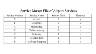
MRP Case 2:
Internation
alAirport
Services
When an aircraft arrives at an international
airport, a towing tractor marshals the aircraft to
an indicated gate. Ramp services and cabin
services are proceeded during the period when
the aircraft stays. Ramp services include the toilet
cleaning, gas refueling, etc. Cabin services
include catering load, garbage dumping, etc.
Figure is a simplified aircraft Material
Requirement Planning
Since the times for the aircraft arrival and
departure are scheduled, the marshaling services
must be performed at predetermined times. The
other services can be scheduled between the
earliest start time (EST) and the latest start time
(LST) as shown in Figure
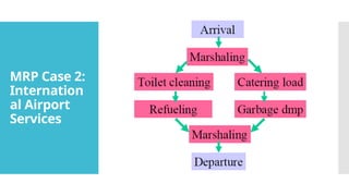
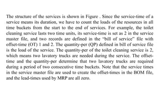
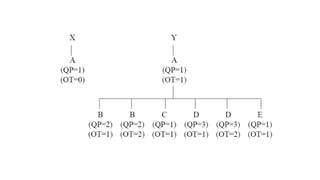
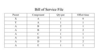
The structure ofthe services is shown in Figure . Since the service-time of a
service means its duration, we have to count the loads of the resources in all
time buckets from the start to the end of services. For example, the toilet
cleaning service lasts two time units, its service-time is set as 2 in the service
master file, and two records are defined in the “bill of service” file with
offset-time (OT) 1 and 2. The quantity-per (QP) defined in bill of service file
is the load of the service. The quantity-per of the toilet cleaning service is 2,
which means two lavatory trucks are needed during the service. The offset-
time and the quantity-per determine that two lavatory trucks are required
during a period of two consecutive time buckets. Note that the service times
in the service master file are used to create the offset-times in the BOM file,
and the lead-times used by MRP are all zero.
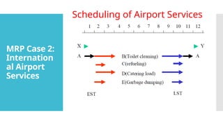
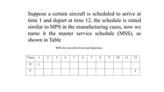
MSS for aircraftarrival and departure
Suppose a certain aircraft is scheduled to arrive at
time 1 and depart at time 12, the schedule is stated
similar to MPS in the manufacturing cases, now we
name it the master service schedule (MSS), as
shown in Table
116.
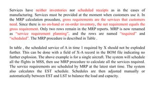
Services have neitherinventories nor scheduled receipts as in the cases of
manufacturing. Services must be provided at the moment when customers use it. In
the MRP calculation procedure, gross requirements are the services that customers
need. Since there is no on-hand or on-order inventory, the net requirement equals the
gross requirement. Only two rows remain in the MRP reports. MRP is now renamed
as “service requirement planning”, and the rows are named “required” and
“scheduled”. The MRP procedure is described in Table .
In table , the scheduled service of A in time 1 required by X should not be exploded
further. This can be done with a field of X-A record in the BOM file indicating no
further explosion. The above example is for a single aircraft. The system will schedule
all the flights in MSS, then use MRP procedure to calculate all the services required.
The service requirements are scheduled by MRP at the latest start time. The system
also calculates the EST schedule. Schedules are then adjusted manually or
automatically between EST and LST to balance the load and capacity.
118.
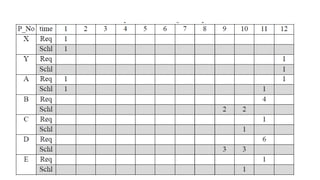
This example explainshow ERP is used in a service business. Time buckets
are sliced as small as the minimal unit a service requires. All service times
are multiple of the time bucket length. Lead-times are all set to 0 because the
start time of the parent operation is exactly the end time of the child
operation, or differs by 1, which can be controlled by offset-time. The
service time determines how many time buckets are needed by an operation.
An operation repeats, as a child item, the required time buckets times, say n,
with offset-time from 1 to n in each BOM record. The service requirement
planning uses the same functions of item master, BOM, MPS, and MRP in
the ERP system. The idea can also be applied to manufacturing operations.
119.
Summary of
MRP
ERPsystem can improve the efficiency of production and
purchasing processes
Efficiency begins with Marketing sharing a sales forecast
Production plan is created based on sales forecast and
shared
with Purchasing so raw materials can be ordered properly
120.
Summary of
MRP
MRPis a…..
Computerized Inventory Control
Production Planning System
that…..
Schedules Component Items as Needed
which will…..
Track Inventory and…..
Help you in many other aspects of business
121.
Thank you foryour
Kind Attention
Dr Gaurang Joshi
Associate Professor
Department of Mechanical engineering
Marwadi University, Rajkot, Gujarat, India
Email:- gaurang.joshi@marwadieducation.edu.in