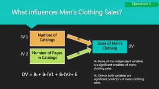
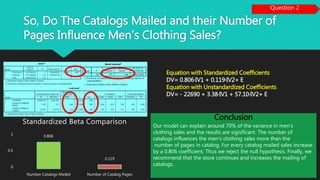
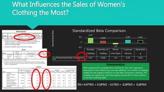
The project analyzes the effects of advertising methods on clothing and jewelry sales from 1989-1999, using SPSS for data processing. It concludes that the number of catalogs mailed significantly influences men's clothing sales, explaining 70% of variance, while adding phone lines increased the explanation to 78%. For women's clothing, the number of catalogs mailed has the highest influence, with variables explaining around 66% of sales variance.

1. Predictive Analysis
Izmir Vodinaj
MKMR 310
Fall 2015

2. Project Summary
Goal
Determine the effects of the advertising methods on sales of men and women’s clothing and jewelry.
Data Used (All variables of interest)
1989 -1999 number of catalogs and their pages, phone lines, and men’s and women’s clothing sales.
SPSS Procedures Used
Frequencies, Regression, Select Files, Split File and Graph.
Potential Insights
Determination of continuation of catalog mailing and segmented target content.

3. What influences Men’s Clothing Sales?
Number of
Catalogs
Number of Pages
in Catalogs
Sales of Men’s
Clothing
IV 1
IV 2
DV
DV = B0 + B1*IV1 + B2*IV2+ E
H0: None of the independent variables
is a significant predictor of men’s
clothing sales.
Ha: One or both variables are
significant predictors of men’s clothing
sales.
Question 1

4. Regression Assumptions: Number of Mailed
Catalogs and Catalog Pages
Continuous Variables
Normal Distribution
Linear Relationships
No Multicolinearity
No influential cases

5. Data Frequencies
Question 1
Interpretation
Looking at the skewnesses of these
variables all being less than 3 and
the kurtoses being less than 8, we
are able to determine that the
variables under study are normally
distributed. Furthermore, looking at
the individual variables we also see
that they are continuous.
Continuous Variables
Normal Distribution
Linear Relationships
No Multicolinearity
No influential cases

6. Checking Linearity
Difference between
R Squares is > 0.03 Difference between
R Squares is < 0.03
While number of pages in a catalog
and the Men’s clothing sales have
a linear relationship, the number of
catalogs mailed and men’s clothing
sales do not have a linear
relationship. This could potentially
be a sign that the linear model may
not be the best model for this project.
Continuous Variables
Normal Distribution
Linear Relationships Partially
No Multicolinearity
No influential cases
Question 2

7. Checking Multicolinearity
Tolerance > 0.2
VIF < 5
Continuous Variables
Normal Distribution
Linear Relationships Partially
No Multicolinearity
No influential cases
Due to our tolerance greater
Than 0.2 and the variance
Inflation factor smaller than 5,
We determine that there is no
Multicolinearity.
Question 2

8. Checking for Influential Cases
Before the Influential Case has been deleted:
I
II
After the Influential Case has been deleted:
Continuous Variables
Normal Distribution
Linear Relationships Partially
No Multicolinearity
No influential cases One Deleted
One influential case was found, and it
was deleted. After its deletion, the R
Square and the Adjusted R Square
resulted higher while remaining
significant. Beta Coefficients on the
other hand changed in different
directions. The coef. For number of
catalogs increased while the coef. For
the number of pages in a catalog
decreased.
Question 2

9. So, Do The Catalogs Mailed and their Number of
Pages Influence Men’s Clothing Sales?
Question 2
Equation with Standardized Coefficients
DV= 0.806*IV1 + 0.119*IV2+ E
Equation with Unstandardized Coefficients
DV= - 22690 + 3.38*IV1 + 57.10*IV2+ E
Conclusion
Our model can explain around 70% of the variance in men’s
clothing sales and the results are significant. The number of
catalogs influences the men’s clothing sales more than the
number of pages in catalog. For every catalog mailed sales increase
by a 0.806 coefficient. Thus we reject the null hypothesis. Finally, we
recommend that the store continues and increases the mailing of
catalogs.
0.806
0.119
0
0.5
1
Number Catalogs Mailed Number of Catalog Pages
Standardized Beta Comparison

10. What influences Men’s Clothing Sales?
Number of
Catalogs
Number of Pages
in Catalogs Sales of Men’s
Clothing
B2
IV 1
IV 2
DV
DV = B0 + B1*IV1 + B2*IV2+ B3*IV3 + E
H0: Adding open phone lines as an
independent variable does no
change the explanation of
variance of men’s clothing sales.
Ha: Adding open phone lines as an
independent variable does change
the explanation of variance of
men’s clothing sales.
Question 3
Number of Pages
in Catalogs
IV 3

11. Regression Assumptions: Phone Lines Added
Continuous Variables
Normal Distribution
Linear Relationships
No Multicolinearity
No influential cases
Question 3

12. Data Frequencies
Question 3
Interpretation
Looking at the skewnesses of these
variables all being less than 3 and
the kurtoses being less than 8, we
are able to determine that the
variables under study are normally
distributed. Furthermore, looking at
the individual variables we also see
that they are continuous.
Continuous Variables
Normal Distribution
Linear Relationships
No Multicolinearity
No influential cases

13. Checking Linearity
Difference between
R Squares is < 0.03
Difference between
R Squares is < 0.03
Adding the phone lines has made it possible
that all of the independent variables have
linear relationship because the differences
between R Squares are under 3%.
Continuous Variables
Normal Distribution
Linear Relationships
No Multicolinearity
No influential cases
Question 3
Difference between
R Squares is < 0.03

14. Checking Multicolinearity
Tolerance > 0.2
VIF < 5
Continuous Variables
Normal Distribution
Linear Relationships
No Multicolinearity
No influential cases
Due to our tolerance greater
than 0.2 and the variance
inflation factors smaller than 5,
we determine that there is no
multicolinearity.
Question 3

15. Checking for Influential Cases
Before the potential Influential Case has been deleted:
I
II
After the potential Influential Case has been deleted:
Continuous Variables
Normal Distribution
Linear Relationships Partially
No Multicolinearity
No influential cases
No influential cases were found. After
suspecting for one influential case
and deleting it, the R Square and the
Adjusted R Square resulted lower
while remaining significant. Beta
Coefficients also decreased with the
removal of the suspected influential
case.
Question 3

16. So, does the addition of open phone lines change
the results?
Question 3
Equation with Standardized Coefficients
DV= 0.523*IV1 + 0.110*IV2 + 0.431*IV3 + E
Equation with Unstandardized Coefficients
DV= - 19041 + 1.95*IV1 + 53.5*IV2+ 322.3*IV3 + E
Conclusion
Our model can explain around 78% of the variance in men’s
clothing sales, and the results are significant. Adding the phone lines
increased the explanation by more than 7%. The number of catalogs
still have the highest influence on men’s clothing sales, yet open
phone lines have a huge significance as well. For every catalog
mailed sales increase by a 0.523 coefficient while for every open
phone line sales increase by a 0.431 coefficient. Thus we reject the
null hypothesis. Finally, we recommend that the store continues and
increases the mailing of catalogs and open new phone lines.
0.523
0.11
0.431
0
0.2
0.4
0.6
Number Catalogs
Mailed
Number of Catalog
Pages
Phone Lines Open
Standardized Beta Comparison

17. Comparing the first 5 years to the last 5 years
Number of Catalogs
Number of Pages in
Catalogs
Sales of Men’s
ClothingB2
IV 1
IV 2
DV
DV = B0 + B1*IV1 + B2*IV2+ B3*IV3 + E
H0: The explanation of the variance
and the significance do not change
from the first five years (1989 –
1993) to the last five years (1994 –
1999).
Ha: The explanation of the variance
and the significance does change
from the first five years (1989 –
1993) to the last five years (1994 –
1999).
Question 3
Number of Pages in
Catalogs
IV 3
Year
Differences
B2

18. Question 3
0.735
0.752
1989 - 1993 1994 - 1999
Adjusted R Square
1989 - 1993 1994 - 1999
1989 – 1993: St DV= 0.596*IV1 + 0.005*IV2 + 0.407*IV3
Unstandardized DV= - 20423 + 2.6*IV1 + 1.8*IV2+ 321.2*IV3 + E
1994 – 1999: St DV= 0.525*IV1 + 0.162*IV2 + 0.470*IV3 + E
Unstandardized DV= - 26740 + 1.98*IV1 + 80.5*IV2+ 435.4*IV3 + E
Do the first 5 years differ the last 5 years?
Conclusion
The variance of explanation differs between the years of 1989 – 1993
and 1994 - 1999 with a slightly higher variance of explanation.
Number of catalog pages has no significance during the first five years
and its beta coefficient increases during the second five years. The
open phone lines have a higher beta coefficient during the second five
years also, yet the number of catalogs beta coefficient decreased during
the second five years. According to these results, we reject our null
hypothesis. Finally, it recommended that the managers of the store
should increase the number of catalogs but pay close attention at the
future trends as its value has been decreasing. In regards to the number
of pages and open phone lines, their data suggests increase in value,
therefore investing in them moderately would be helpful.

19. What Influences the Sales of Women’s
Clothing the Most?
Number
Catalogs…
Number of
Catalog…
Phone
Lines Open
Customer
Service…
Adverstisin
g
Standardized Beta Comparison 0.47 0.184 -0.1 0.29 0.26
0.47
0.184
-0.1
0.29 0.26
-0.5
0
0.5
StandardizedBeta.
Standardized Beta Comparison
Interpretation
After analyzing five variables and checking for the main regression
assumptions (one influencing case was deleted), the number of catalogs
mailed has the highest influence on the sales of women’s clothing. The
variables are significant, and they explain around 66 % of the variance
in women’s clothing sales.
DV= 0.47*IV1 + 0.18*IV2 - 0.1*IV3 + 0.29*IV3 + 0.26*IV3