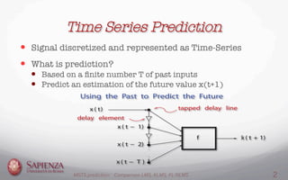
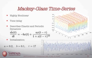
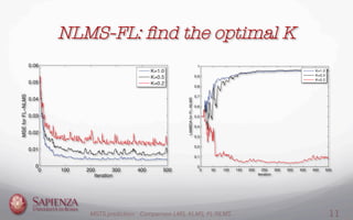
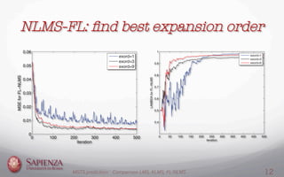
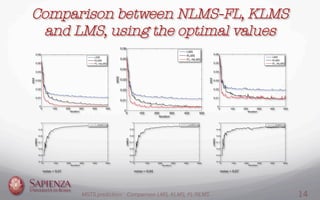
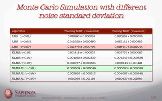
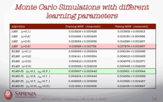
This document compares the LMS, KLMS, and NLMS-FL algorithms for time series prediction on the Mackey-Glass time series. It finds that the NLMS-FL algorithm achieves the best performance with the fastest convergence and lowest mean squared error. Experiments are conducted to determine the optimal parameters for NLMS-FL and compare the performance of the three algorithms under different noise levels and learning rates. The NLMS-FL algorithm outperforms LMS and KLMS in most conditions, demonstrating its effectiveness for time series prediction.

1. Mackey Glass Time Series Prediction:
Comparison between LMS, KLMS and the novel NLMS-FL
Student: Giovanni Murru
Professor: Aurelio Uncini
MGTS prediction: Comparison LMS, KLMS, FL-NLMS 1

2. Time Series Prediction
— Signal discretized and represented as Time-Series
— What is prediction?
— Based on a finite number T of past inputs
— Predict an estimation of the future value x(t+1)
MGTS prediction: Comparison LMS, KLMS, FL-NLMS 2

3. The LMS algorithm
— Based on minimization of the Mean Square Error
J (w) =
N
i=1
(d(i) − wT
u(i)) 2
— Weights are updated following the law:
w(i) = w(i − 1) + ηu(i)( d(i) − w(i − 1)T
u(i
MGTS prediction: Comparison LMS, KLMS, FL-NLMS 3

4. The KLMS algorithm
— Map the input data into a High Dimensional Feature Space.
— Gaussian Kernel:
— Compute the estimated value "
and update the coefficients:
MGTS prediction: Comparison LMS, KLMS, FL-NLMS 4

5. The Functional Link Nonlinear Filter
— An artificial neural network with a single layer
— Creation of Enhanced Input Pattern z[n]
— Adaptive filtering through NLMS algorithm
— Weight Vector:
— Error on the prediction:
— Weight Update Rule:
— Output of the Functional Link Filter:
MGTS prediction: Comparison LMS, KLMS, FL-NLMS 5

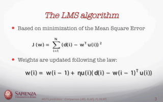
6. Creation of Enhanced Input Pattern
x[1,n]
x[2,n]
x[3,n]
x[Lin,n]
cos( πx[1,n])
sin(2πx[1,n])
cos(5πx[1,n])
sin(6πx[1,n])
cos(3πx[1,n])
sin(4πx[1,n])
1
2*exord =
= 6
cos( πx[Lin,n])
sin(2πx[Lin,n])
cos(5πx[Lin,n])
sin(6πx[Lin,n])
cos(3πx[Lin,n])
sin(4πx[Lin,n])
2*exord * Lin =
= 6*10 = ∆
bias = 1x[n]
z[n]
∆ + bias = 61 = Len
MGTS prediction: Comparison LMS, KLMS, FL-NLMS 6

7. Adaptive Combination: NLMS+FL
— Linear Filter use NLMS:
— Error is computed using a different overall output:
MGTS prediction: Comparison LMS, KLMS, FL-NLMS 7

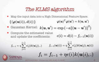
8. A Robust Architecture
— How is the adaptive parameter λ[n] computed?
— It’s computed in function of an adaptive parameter a[n]:
— How is the adaptive parameter a[n] computed?
— It’s computed in function of another adaptive parameter r[n]:
— r[n] is the estimated power of yFL[n]:
MGTS prediction: Comparison LMS, KLMS, FL-NLMS 8

9. 0
100
200
300
400
500
0
2
4
6
8
10
−0.8
−0.6
−0.4
−0.2
0
0.2
0.4
0.6
Mackey-Glass Time-Series
— Highly Nonlinear
— Time delay
— Describes Chaotic and Periodic
Dynamics
— Initialization:
MGTS prediction: Comparison LMS, KLMS, FL-NLMS 9
0 50 100 150 200 250 300 350 400 450 500
−0.8
−0.6
−0.4
−0.2
0
0.2
0.4
0.6

10. Experimental Results
— 2 Classes of Experiments:
— Find optimal parameters for NLMS-FL
— Monte Carlo Simulation on the 3 algorithms
— At different noise
— At different learning parameters
K
µL
µFL
exord MSE
MGTS prediction: Comparison LMS, KLMS, FL-NLMS 10

11. NLMS-FL: find the optimal K
0 100 200 300 400 500
0
0.01
0.02
0.03
0.04
0.05
0.06
iteration
MSEforFL−NLMS
K=1.0
K=0.5
K=0.2
0 50 100 150 200 250 300 350 400 450 500
0
0.1
0.2
0.3
0.4
0.5
0.6
0.7
0.8
0.9
1
iteration
LAMBDAforFL−NLMS
K=1.0
K=0.5
K=0.2
MGTS prediction: Comparison LMS, KLMS, FL-NLMS 11

12. NLMS-FL: find best expansion order
0 100 200 300 400 500
0
0.01
0.02
0.03
0.04
0.05
0.06
iteration
MSEforFL−NLMS
exord=1
exord=3
exord=9
0 50 100 150 200 250 300 350 400 450 500
0.4
0.5
0.6
0.7
0.8
0.9
1
iteration
LAMBDAforFL−NLMS
exord=1
exord=3
exord=9
MGTS prediction: Comparison LMS, KLMS, FL-NLMS 12

13. NLMS-FL: find best learning parameters
0 50 100 150 200 250 300 350 400 450 500
0
0.01
0.02
0.03
0.04
0.05
0.06
iteration
MSEforFL−NLMS
muL=0.1, muNL=0.3
muL=0.3, muNL=0.1
muL=0.7, muNL=0.7
muL=0.01, muNL=0.01
0 50 100 150 200 250 300 350 400 450 500
0
0.01
0.02
0.03
0.04
0.05
0.06
iteration
MSEforFL−NLMS
muL=0.1, muNL=0.3
muL=0.3, muNL=0.1
muL=0.7, muNL=0.7
muL=0.01, muNL=0.01
MGTS prediction: Comparison LMS, KLMS, FL-NLMS 13

14. Comparison between NLMS-FL, KLMS
and LMS, using the optimal values
0 100 200 300 400 500
0.4
0.5
0.6
0.7
0.8
0.9
1
iteration
LAMBDA
LAMBDA
0 100 200 300 400 500
0.4
0.5
0.6
0.7
0.8
0.9
1
iteration
LAMBDA
LAMBDA
0 100 200 300 400 500
0.4
0.5
0.6
0.7
0.8
0.9
1
iteration
LAMBDA
LAMBDA
0 100 200 300 400 500
0
0.01
0.02
0.03
0.04
0.05
0.06
iteration
MSE
LMS
KLMS
FL−NLMS
0 100 200 300 400 500
0
0.01
0.02
0.03
0.04
0.05
0.06
iterationMSE
LMS
KLMS
FL−NLMS
0 100 200 300 400 500
0
0.01
0.02
0.03
0.04
0.05
0.06
iteration
MSE
LMS
KLMS
FL−NLMS
noise = 0.04noise = 0.01 noise = 0.07
MGTS prediction: Comparison LMS, KLMS, FL-NLMS 14

15. Monte Carlo Simulation with different
noise standard deviation
Algorithm
Training MSE (mean±std)
Testing MSE (mean±std)
LMS (σ=0.01)
0.010160 ± 0.000089
0.010659 ± 0.000228
LMS (σ=0.04)
0.012520 ± 0.000480
0.013121 ± 0.000959
LMS (σ=0.07)
0.017379 ± 0.000796
0.018440 ± 0.002044
KLMS (σ=0.01)
0.001818 ± 0.000032
0.001739 ± 0.000087
KLMS (σ=0.04)
0.004160 ± 0.000339
0.004247 ± 0.000536
KLMS (σ=0.07)
0.009077 ± 0.000854
0.009444 ± 0.001421
NLMS-FL (σ=0.01)
0.000509 ± 0.000049
0.000550 ± 0.000099
NLMS-FL (σ=0.04)
0.003655 ± 0.000513
0.004057 ± 0.000842
NLMS-FL (σ=0.07)
0.010059 ± 0.001116
0.010637 ± 0.001967
MGTS prediction: Comparison LMS, KLMS, FL-NLMS 15

16. Monte Carlo Simulations with different
learning parameters
Algorithm
Training MSE (mean±std)
Testing MSE (mean±std)
LMS (µ=0.1)
0.013209 ± 0.000426
0.013902 ± 0.000913
LMS (µ=0.2)
0.012495 ± 0.000435
0.013130 ± 0.000966
LMS (µ=0.6)
0.013634 ± 0.000936
0.014326 ± 0.001267
LMS (µ=0.9)
0.016525 ± 0.001752
0.017279 ± 0.001967
KLMS (µ=0.1)
0.005959 ± 0.000204
0.006194 ± 0.000496
KLMS (µ=0.2)
0.004141 ± 0.000334
0.004213 ± 0.000453
KLMS (µ=0.6)
0.004210 ± 0.001276
0.004372 ± 0.001571
KLMS (µ=0.9)
0.005599 ± 0.002009
0.005498 ± 0.002065
NLMS-FL (µL=0.1, µNL=0.3 )
0.003647 ± 0.000440
0.003901 ± 0.000644
NLMS-FL (µL=0.3, µNL=0.1 )
0.004204 ± 0.000443
0.004562 ± 0.000656
NLMS-FL (µL=0.7, µNL=0.7 )
0.009653 ± 0.003956
0.010526 ± 0.004457
NLMS-FL (µL=0.01, µNL=0.01)
0.011550 ± 0.000308
0.012106 ± 0.000847
MGTS prediction: Comparison LMS, KLMS, FL-NLMS 16

17. Conclusion and Results
— NLMS-FL is the best performer!
— Great difference in performance at low noise!
— Very Rapid Convergence of the learning curve!
High Speed of Adaptation!
— Monte Carlo simulation confirms the results as
regard the best learning parameters!
— KLMS is still a good solution. LMS is not enough.
MGTS prediction: Comparison LMS, KLMS, FL-NLMS 17

18. Thanks for
Your Attention!"
References:
[1] D.Comminiello, A.Uncini, R. Parisi and
M.Scarpiniti, A Functional Link Based
Nonlinear Echo Canceller Exploiting
Sparsity.
[2] D.Comminiello, A.Uncini, M.Scarpiniti,
L.A.Azpicueta-Ruiz and J.Arenas-Garcia,
Functional Link Based Architectures For
Nonlinear Acoustic Echo Cancellation.
[3] Y.H.Pao, Adaptive Pattern Recognition
and Neural Networks.
[4] A.Uncini, Neural Networks:
Computational and Biological Inspired
Intelligent Circuits.
[5] Weifeng Liu, Jose C. Principe, and Simon
Haykin, Kernel Adaptive Filtering:
A Comprehensive Introduction.
[6] Dave Touretzky and Kornel Laskowski,
15-486/782: Artificial Neural Network, FALL
2006, Neural Networks for Time Series
Prediction.
MGTS prediction: Comparison LMS, KLMS, FL-NLMS 18