Machine Leaning unit 02

1. Data preparation
Data preparation is a crucial step in machine learning, involving the transformation and preprocessing of raw data
to make it suitable for model training. This process ensures that the data is clean, consistent, and relevant, which
ultimately improves the performance and reliability of machine learning models. Data preparation typically
involves several key steps:
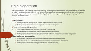
1.Data Cleaning:
1. Identify and handle missing values, outliers, and inconsistencies in the dataset.
2. Techniques include imputation, removing duplicates, and correcting errors.
2.Feature Selection and Engineering:
1. Select relevant features that contribute most to the predictive task.
2. Create new features from existing ones to capture additional information.
3. Techniques include correlation analysis, dimensionality reduction, and domain knowledge incorporation.
3.Data Scaling and Normalization:
1. Scale features to a similar range to prevent certain features from dominating others.
2. Normalize data to have a standard distribution, improving convergence and performance.
3. Techniques include min-max scaling, standardization, and robust scaling.

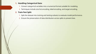
2. 1. Handling Categorical Data:
1. Convert categorical variables into a numerical format suitable for modeling.
2. Techniques include one-hot encoding, label encoding, and target encoding.
2. Train-Test Split:
1. Split the dataset into training and testing subsets to evaluate model performance.
2. Ensure the preservation of data distribution across splits to prevent bias.

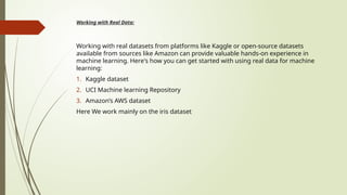
3. Working with Real Data:
Working with real datasets from platforms like Kaggle or open-source datasets
available from sources like Amazon can provide valuable hands-on experience in
machine learning. Here's how you can get started with using real data for machine
learning:
1. Kaggle dataset
2. UCI Machine learning Repository
3. Amazon’s AWS dataset
Here We work mainly on the iris dataset

5. IRIS Flower Types

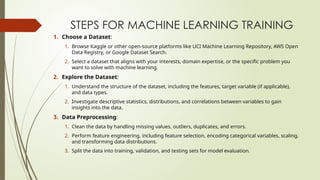
6. STEPS FOR MACHINE LEARNING TRAINING
1. Choose a Dataset:
1. Browse Kaggle or other open-source platforms like UCI Machine Learning Repository, AWS Open
Data Registry, or Google Dataset Search.
2. Select a dataset that aligns with your interests, domain expertise, or the specific problem you
want to solve with machine learning.
2. Explore the Dataset:
1. Understand the structure of the dataset, including the features, target variable (if applicable),
and data types.
2. Investigate descriptive statistics, distributions, and correlations between variables to gain
insights into the data.
3. Data Preprocessing:
1. Clean the data by handling missing values, outliers, duplicates, and errors.
2. Perform feature engineering, including feature selection, encoding categorical variables, scaling,
and transforming data distributions.
3. Split the data into training, validation, and testing sets for model evaluation.

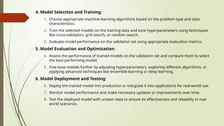
7. 4. Model Selection and Training:
1. Choose appropriate machine learning algorithms based on the problem type and data
characteristics.
2. Train the selected models on the training data and tune hyperparameters using techniques
like cross-validation, grid search, or random search.
3. Evaluate model performance on the validation set using appropriate evaluation metrics.
5. Model Evaluation and Optimization:
4. Assess the performance of trained models on the validation set and compare them to select
the best-performing model.
5. Fine-tune models further by adjusting hyperparameters, exploring different algorithms, or
applying advanced techniques like ensemble learning or deep learning.
6. Model Deployment and Testing:
6. Deploy the trained model into production or integrate it into applications for real-world use.
7. Monitor model performance and make necessary updates or improvements over time.
8. Test the deployed model with unseen data to ensure its effectiveness and reliability in real-
world scenarios.

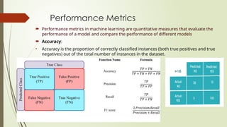
8. Performance Metrics
 Performance metrics in machine learning are quantitative measures that evaluate the
performance of a model and compare the performance of different models
 Accuracy:
• Accuracy is the proportion of correctly classified instances (both true positives and true
negatives) out of the total number of instances in the dataset.

9. Get the Data(choose the data)
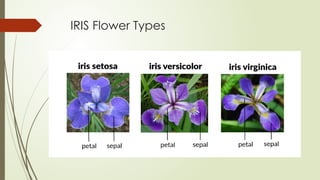
 The Iris dataset is a popular dataset often used for machine learning
classification tasks. It consists of 150 samples of iris flowers, each with four
features (sepal length, sepal width, petal length, and petal width) and a
corresponding target variable representing the species of the iris flower (setosa,
versicolor, or virginica). Here's how you can obtain the Iris dataset for machine
learning:
 Using Scikit-Learn:
• Scikit-learn, a popular machine learning library in Python, provides easy access to
the Iris dataset through its datasets module.
• You can load the Iris dataset using the load_iris() function:

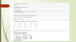
10. 1. Load the Data: Start by loading your dataset into your preferred data analysis environment such as Python with libraries like
Pandas, NumPy, and Matplotlib/Seaborn for visualization.
2. Basic Data Exploration:
 Check the first few rows of the dataset using the .head() function to understand its structure.
 Check the dimensions of the dataset (number of rows and columns) using the .shape attribute.
 Use the .info() function to get a concise summary of the dataset, including data types and missing values.
 Compute summary statistics such as mean, median, standard deviation, minimum, and maximum values for numerical
features using the .describe() function.
 For categorical features, you can use the .value_counts() function to get the frequency distribution of unique values.

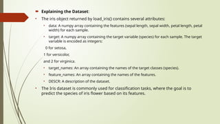
12.  Explaining the Dataset:
• The iris object returned by load_iris() contains several attributes:
• data: A numpy array containing the features (sepal length, sepal width, petal length, petal
width) for each sample.
• target: A numpy array containing the target variable (species) for each sample. The target
variable is encoded as integers:
0 for setosa,
1 for versicolor,
and 2 for virginica.
• target_names: An array containing the names of the target classes (species).
• feature_names: An array containing the names of the features.
• DESCR: A description of the dataset.
• The Iris dataset is commonly used for classification tasks, where the goal is to
predict the species of iris flower based on its features.

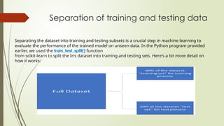
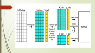
14. Separation of training and testing data
Separating the dataset into training and testing subsets is a crucial step in machine learning to
evaluate the performance of the trained model on unseen data. In the Python program provided
earlier, we used the train_test_split() function
from scikit-learn to split the Iris dataset into training and testing sets. Here's a bit more detail on
how it works:

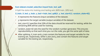
16. from sklearn.model_selection import train_test_split
# Split the data into training and testing sets (80% train, 20% test)
X_train, X_test, y_train, y_test = train_test_split(X, y, test_size=0.2, random_state=42)
• X represents the features (input variables) of the dataset.
• y represents the target variable (output variable) of the dataset.
• test_size=0.2 specifies that 20% of the data should be reserved for testing, while the
remaining 80% will be used for training.
• random_state=42 sets the seed for the random number generator. This ensures
reproducibility so that each time you run the code, you get the same split of data.
 After splitting, X_train and y_train contain the features and target variable for the
training set, respectively, while X_test and y_test contain the features and target
variable for the testing set, respectively.

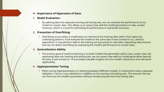
17.  Importance of Separation of Data:
1. Model Evaluation:
1. By splitting data into separate training and testing sets, we can evaluate the performance of our
model on unseen data. This allows us to assess how well the model generalizes to new, unseen
instances, which is crucial for estimating its performance in real-world scenarios.
2. Prevention of Overfitting:
1. Overfitting occurs when a model learns to memorize the training data rather than capturing
underlying patterns. If we evaluate the model on the same data it was trained on (i.e., without
separation), it may perform well on the training set but poorly on new data. Separating data ensures
that we can detect overfitting by evaluating the model's performance on unseen data.
3. Generalization Ability:
1. The primary goal of machine learning is to build models that generalize well to new, unseen data. By
separating data into training and testing sets, we can assess how well our model generalizes beyond
the data it was trained on. This provides valuable insights into the model's robustness and real-world
applicability.
4. Hyperparameter Tuning:
1. When tuning hyperparameters or selecting between different models, it's essential to have a separate
validation n set (or cross-validation) in addition to the training and testing sets. This ensures that we
can fine-tune the model's parameters without introducing bias from the testing data.

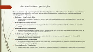
18. data visualization to gain insights
These visualizations help us gain insights into the relationships between different features in the dataset and understand
how they contribute. Visualizing data in this way can aid in feature selection, model building, and understanding the
underlying patterns in the data.
1. Exploratory Data Analysis (EDA):
1. Visualizing data distributions, outliers, and patterns helps understand the dataset's characteristics and identify potential data
quality issues.
2. Feature Importance Visualization:
1. Visualizing feature importance scores using plots like bar charts or heatmaps helps identify influential features in predictive
models.
3. Model Performance Visualization:
1. Visualizing performance metrics such as accuracy, precision, recall, and F1-score using ROC curves, precision-recall curves, or
confusion matrices provides insights into model performance.
4. Model Interpretability Visualization:
1. Visualizing individual model predictions and decision boundaries using partial dependence plots, SHAP plots, or LIME
visualizations aids in model interpretation.
5. Feature Relationship Visualization:
1. Visualizing relationships between features using scatter plots, correlation matrices, or heatmaps uncovers multicollinearity and
identifies correlated feature groups.
6. Anomaly Detection Visualization:
1. Visualizing anomalies or outliers using scatter plots or box plots helps identify unusual patterns requiring further investigation.

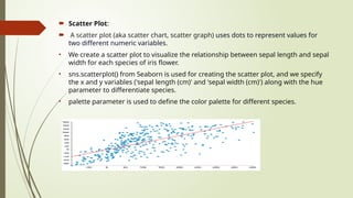
19.  Scatter Plot:
 A scatter plot (aka scatter chart, scatter graph) uses dots to represent values for
two different numeric variables.
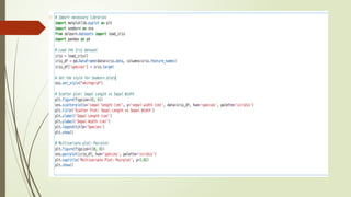
• We create a scatter plot to visualize the relationship between sepal length and sepal
width for each species of iris flower.
• sns.scatterplot() from Seaborn is used for creating the scatter plot, and we specify
the x and y variables ('sepal length (cm)' and 'sepal width (cm)') along with the hue
parameter to differentiate species.
• palette parameter is used to define the color palette for different species.

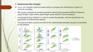
20.  Multivariate Plot: Pairplot:
 A pair plot creates a grid of scatter plots to compare the distribution of pairs of
numeric variables.
• We create a pairplot to visualize pairwise relationships between different features
(sepal length, sepal width, petal length, petal width) in the Iris dataset.
• sns.pairplot() from Seaborn is used to create the pairplot, and we specify the hue
parameter to differentiate species.
• This plot provides a quick overview of the relationships between all pairs of variables
in the dataset.

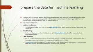
22. prepare the data for machine learning
 Preparing data for machine learning algorithms involves several steps to ensure that the dataset is formatted
correctly, features are appropriately scaled, and the data is ready to be used for training a model. Here's a
comprehensive guide to preparing data for machine learning:
 Explanation of the code:
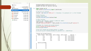
1. Load the Iris Dataset:
1. We load the Iris dataset from a CSV file using pd.read_csv(). Make sure to adjust the filename according to your
dataset file.
2. Data Cleaning:
1. We remove duplicate rows from the dataset using the drop_duplicates() method. This ensures that each
observation is unique.
3. Label Encoding:
1. We use LabelEncoder from scikit-learn to convert the categorical variable 'species' into numerical labels. This is
necessary because machine learning models typically require numerical input.
2. fit_transform() method is used to fit the label encoder on the 'species' column and transform it into numerical
labels. The encoded labels are stored in a new column 'species_encoded'.

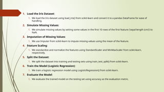
24. 1. Load the Iris Dataset:
1. We load the Iris dataset using load_iris() from scikit-learn and convert it to a pandas DataFrame for ease of
handling.
2. Simulate Missing Values:
1. We simulate missing values by setting some values in the first 10 rows of the first feature ('sepal length (cm)') to
NaN.
3. Imputation of Missing Values:
1. We use Imputer from scikit-learn to impute missing values using the mean of the feature.
4. Feature Scaling:
1. We standardize and normalize the features using StandardScaler and MinMaxScaler from scikit-learn,
respectively.
5. Split the Dataset:
1. We split the dataset into training and testing sets using train_test_split() from scikit-learn.
6. Train the Model (Logistic Regression):
1. We train a logistic regression model using LogisticRegression() from scikit-learn.
7. Evaluate the Model:
1. We evaluate the trained model on the testing set using accuracy as the evaluation metric.