This document is the preface to the book "Introduction to Machine Learning with Python" by Andreas C. Müller and Sarah Guido. The preface provides an overview of the book, including who it is intended for, why the authors wrote it, how it is organized, and conventions used. It is an introductory book on machine learning using Python and scikit-learn that requires no previous experience, focusing on practical applications rather than advanced mathematics.
![978-1-449-36941-5
[LSI]
Introduction to Machine Learning with Python
by Andreas C. Müller and Sarah Guido
Copyright © 2017 Sarah Guido, Andreas Müller. All rights reserved.
Printed in the United States of America.
Published by O’Reilly Media, Inc., 1005 Gravenstein Highway North, Sebastopol, CA 95472.
O’Reilly books may be purchased for educational, business, or sales promotional use. Online editions are
also available for most titles (http://safaribooksonline.com). For more information, contact our corporate/
institutional sales department: 800-998-9938 or corporate@oreilly.com.
Editor: Dawn Schanafelt
Production Editor: Kristen Brown
Copyeditor: Rachel Head
Proofreader: Jasmine Kwityn
Indexer: Judy McConville
Interior Designer: David Futato
Cover Designer: Karen Montgomery
Illustrator: Rebecca Demarest
October 2016: First Edition
Revision History for the First Edition
2016-09-22: First Release
See http://oreilly.com/catalog/errata.csp?isbn=9781449369415 for release details.
The O’Reilly logo is a registered trademark of O’Reilly Media, Inc. Introduction to Machine Learning with
Python, the cover image, and related trade dress are trademarks of O’Reilly Media, Inc.
While the publisher and the authors have used good faith efforts to ensure that the information and
instructions contained in this work are accurate, the publisher and the authors disclaim all responsibility
for errors or omissions, including without limitation responsibility for damages resulting from the use of
or reliance on this work. Use of the information and instructions contained in this work is at your own
risk. If any code samples or other technology this work contains or describes is subject to open source
licenses or the intellectual property rights of others, it is your responsibility to ensure that your use
thereof complies with such licenses and/or rights.](https://image.slidesharecdn.com/introductiontomachinelearningwithpythonpdfdrive-230107170822-bfb01dbd/85/Introduction-to-Machine-Learning-with-Python-PDFDrive-com-pdf-4-320.jpg)


![1 If you are unfamiliar with NumPy or matplotlib, we recommend reading the first chapter of the SciPy Lec‐
ture Notes.
If you already have a Python installation set up, you can use pip to install all of these
packages:
$ pip install numpy scipy matplotlib ipython scikit-learn pandas
Essential Libraries and Tools
Understanding what scikit-learn is and how to use it is important, but there are a
few other libraries that will enhance your experience. scikit-learn is built on top of
the NumPy and SciPy scientific Python libraries. In addition to NumPy and SciPy, we
will be using pandas and matplotlib. We will also introduce the Jupyter Notebook,
which is a browser-based interactive programming environment. Briefly, here is what
you should know about these tools in order to get the most out of scikit-learn.1
Jupyter Notebook
The Jupyter Notebook is an interactive environment for running code in the browser.
It is a great tool for exploratory data analysis and is widely used by data scientists.
While the Jupyter Notebook supports many programming languages, we only need
the Python support. The Jupyter Notebook makes it easy to incorporate code, text,
and images, and all of this book was in fact written as a Jupyter Notebook. All of the
code examples we include can be downloaded from GitHub.
NumPy
NumPy is one of the fundamental packages for scientific computing in Python. It
contains functionality for multidimensional arrays, high-level mathematical func‐
tions such as linear algebra operations and the Fourier transform, and pseudorandom
number generators.
In scikit-learn, the NumPy array is the fundamental data structure. scikit-learn
takes in data in the form of NumPy arrays. Any data you’re using will have to be con‐
verted to a NumPy array. The core functionality of NumPy is the ndarray class, a
multidimensional (n-dimensional) array. All elements of the array must be of the
same type. A NumPy array looks like this:
In[2]:
import numpy as np
x = np.array([[1, 2, 3], [4, 5, 6]])
print("x:n{}".format(x))
Essential Libraries and Tools | 7](https://image.slidesharecdn.com/introductiontomachinelearningwithpythonpdfdrive-230107170822-bfb01dbd/85/Introduction-to-Machine-Learning-with-Python-PDFDrive-com-pdf-21-320.jpg)
![Out[2]:
x:
[[1 2 3]
[4 5 6]]
We will be using NumPy a lot in this book, and we will refer to objects of the NumPy
ndarray class as “NumPy arrays” or just “arrays.”
SciPy
SciPy is a collection of functions for scientific computing in Python. It provides,
among other functionality, advanced linear algebra routines, mathematical function
optimization, signal processing, special mathematical functions, and statistical distri‐
butions. scikit-learn draws from SciPy’s collection of functions for implementing
its algorithms. The most important part of SciPy for us is scipy.sparse: this provides
sparse matrices, which are another representation that is used for data in scikit-
learn. Sparse matrices are used whenever we want to store a 2D array that contains
mostly zeros:
In[3]:
from scipy import sparse
# Create a 2D NumPy array with a diagonal of ones, and zeros everywhere else
eye = np.eye(4)
print("NumPy array:n{}".format(eye))
Out[3]:
NumPy array:
[[ 1. 0. 0. 0.]
[ 0. 1. 0. 0.]
[ 0. 0. 1. 0.]
[ 0. 0. 0. 1.]]
In[4]:
# Convert the NumPy array to a SciPy sparse matrix in CSR format
# Only the nonzero entries are stored
sparse_matrix = sparse.csr_matrix(eye)
print("nSciPy sparse CSR matrix:n{}".format(sparse_matrix))
Out[4]:
SciPy sparse CSR matrix:
(0, 0) 1.0
(1, 1) 1.0
(2, 2) 1.0
(3, 3) 1.0
8 | Chapter 1: Introduction](https://image.slidesharecdn.com/introductiontomachinelearningwithpythonpdfdrive-230107170822-bfb01dbd/85/Introduction-to-Machine-Learning-with-Python-PDFDrive-com-pdf-22-320.jpg)
![Usually it is not possible to create dense representations of sparse data (as they would
not fit into memory), so we need to create sparse representations directly. Here is a
way to create the same sparse matrix as before, using the COO format:
In[5]:
data = np.ones(4)
row_indices = np.arange(4)
col_indices = np.arange(4)
eye_coo = sparse.coo_matrix((data, (row_indices, col_indices)))
print("COO representation:n{}".format(eye_coo))
Out[5]:
COO representation:
(0, 0) 1.0
(1, 1) 1.0
(2, 2) 1.0
(3, 3) 1.0
More details on SciPy sparse matrices can be found in the SciPy Lecture Notes.
matplotlib
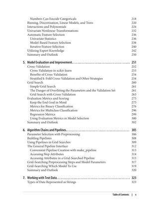
matplotlib is the primary scientific plotting library in Python. It provides functions
for making publication-quality visualizations such as line charts, histograms, scatter
plots, and so on. Visualizing your data and different aspects of your analysis can give
you important insights, and we will be using matplotlib for all our visualizations.
When working inside the Jupyter Notebook, you can show figures directly in the
browser by using the %matplotlib notebook and %matplotlib inline commands.
We recommend using %matplotlib notebook, which provides an interactive envi‐
ronment (though we are using %matplotlib inline to produce this book). For
example, this code produces the plot in Figure 1-1:
In[6]:
%matplotlib inline
import matplotlib.pyplot as plt
# Generate a sequence of numbers from -10 to 10 with 100 steps in between
x = np.linspace(-10, 10, 100)
# Create a second array using sine
y = np.sin(x)
# The plot function makes a line chart of one array against another
plt.plot(x, y, marker="x")
Essential Libraries and Tools | 9](https://image.slidesharecdn.com/introductiontomachinelearningwithpythonpdfdrive-230107170822-bfb01dbd/85/Introduction-to-Machine-Learning-with-Python-PDFDrive-com-pdf-23-320.jpg)
![Figure 1-1. Simple line plot of the sine function using matplotlib
pandas
pandas is a Python library for data wrangling and analysis. It is built around a data
structure called the DataFrame that is modeled after the R DataFrame. Simply put, a
pandas DataFrame is a table, similar to an Excel spreadsheet. pandas provides a great
range of methods to modify and operate on this table; in particular, it allows SQL-like
queries and joins of tables. In contrast to NumPy, which requires that all entries in an
array be of the same type, pandas allows each column to have a separate type (for
example, integers, dates, floating-point numbers, and strings). Another valuable tool
provided by pandas is its ability to ingest from a great variety of file formats and data‐
bases, like SQL, Excel files, and comma-separated values (CSV) files. Going into
detail about the functionality of pandas is out of the scope of this book. However,
Python for Data Analysis by Wes McKinney (O’Reilly, 2012) provides a great guide.
Here is a small example of creating a DataFrame using a dictionary:
In[7]:
import pandas as pd
# create a simple dataset of people
data = {'Name': ["John", "Anna", "Peter", "Linda"],
'Location' : ["New York", "Paris", "Berlin", "London"],
'Age' : [24, 13, 53, 33]
}
data_pandas = pd.DataFrame(data)
# IPython.display allows "pretty printing" of dataframes
# in the Jupyter notebook
display(data_pandas)
10 | Chapter 1: Introduction](https://image.slidesharecdn.com/introductiontomachinelearningwithpythonpdfdrive-230107170822-bfb01dbd/85/Introduction-to-Machine-Learning-with-Python-PDFDrive-com-pdf-24-320.jpg)
![This produces the following output:
Age Location Name
0 24 New York John
1 13 Paris Anna
2 53 Berlin Peter
3 33 London Linda
There are several possible ways to query this table. For example:
In[8]:
# Select all rows that have an age column greater than 30
display(data_pandas[data_pandas.Age > 30])
This produces the following result:
Age Location Name
2 53 Berlin Peter
3 33 London Linda
mglearn
This book comes with accompanying code, which you can find on GitHub. The
accompanying code includes not only all the examples shown in this book, but also
the mglearn library. This is a library of utility functions we wrote for this book, so
that we don’t clutter up our code listings with details of plotting and data loading. If
you’re interested, you can look up all the functions in the repository, but the details of
the mglearn module are not really important to the material in this book. If you see a
call to mglearn in the code, it is usually a way to make a pretty picture quickly, or to
get our hands on some interesting data.
Throughout the book we make ample use of NumPy, matplotlib
and pandas. All the code will assume the following imports:
import numpy as np
import matplotlib.pyplot as plt
import pandas as pd
import mglearn
We also assume that you will run the code in a Jupyter Notebook
with the %matplotlib notebook or %matplotlib inline magic
enabled to show plots. If you are not using the notebook or these
magic commands, you will have to call plt.show to actually show
any of the figures.
Essential Libraries and Tools | 11](https://image.slidesharecdn.com/introductiontomachinelearningwithpythonpdfdrive-230107170822-bfb01dbd/85/Introduction-to-Machine-Learning-with-Python-PDFDrive-com-pdf-25-320.jpg)
![2 The six package can be very handy for that.
Python 2 Versus Python 3
There are two major versions of Python that are widely used at the moment: Python 2
(more precisely, 2.7) and Python 3 (with the latest release being 3.5 at the time of
writing). This sometimes leads to some confusion. Python 2 is no longer actively
developed, but because Python 3 contains major changes, Python 2 code usually does
not run on Python 3. If you are new to Python, or are starting a new project from
scratch, we highly recommend using the latest version of Python 3 without changes.
If you have a large codebase that you rely on that is written for Python 2, you are
excused from upgrading for now. However, you should try to migrate to Python 3 as
soon as possible. When writing any new code, it is for the most part quite easy to
write code that runs under Python 2 and Python 3.2
If you don’t have to interface with
legacy software, you should definitely use Python 3. All the code in this book is writ‐
ten in a way that works for both versions. However, the exact output might differ
slightly under Python 2.
Versions Used in this Book
We are using the following versions of the previously mentioned libraries in this
book:
In[9]:
import sys
print("Python version: {}".format(sys.version))
import pandas as pd
print("pandas version: {}".format(pd.__version__))
import matplotlib
print("matplotlib version: {}".format(matplotlib.__version__))
import numpy as np
print("NumPy version: {}".format(np.__version__))
import scipy as sp
print("SciPy version: {}".format(sp.__version__))
import IPython
print("IPython version: {}".format(IPython.__version__))
import sklearn
print("scikit-learn version: {}".format(sklearn.__version__))
12 | Chapter 1: Introduction](https://image.slidesharecdn.com/introductiontomachinelearningwithpythonpdfdrive-230107170822-bfb01dbd/85/Introduction-to-Machine-Learning-with-Python-PDFDrive-com-pdf-26-320.jpg)
![Out[9]:
Python version: 3.5.2 |Anaconda 4.1.1 (64-bit)| (default, Jul 2 2016, 17:53:06)
[GCC 4.4.7 20120313 (Red Hat 4.4.7-1)]
pandas version: 0.18.1
matplotlib version: 1.5.1
NumPy version: 1.11.1
SciPy version: 0.17.1
IPython version: 5.1.0
scikit-learn version: 0.18
While it is not important to match these versions exactly, you should have a version
of scikit-learn that is as least as recent as the one we used.
Now that we have everything set up, let’s dive into our first application of machine
learning.
This book assumes that you have version 0.18 or later of scikit-
learn. The model_selection module was added in 0.18, and if you
use an earlier version of scikit-learn, you will need to adjust the
imports from this module.
A First Application: Classifying Iris Species
In this section, we will go through a simple machine learning application and create
our first model. In the process, we will introduce some core concepts and terms.
Let’s assume that a hobby botanist is interested in distinguishing the species of some
iris flowers that she has found. She has collected some measurements associated with
each iris: the length and width of the petals and the length and width of the sepals, all
measured in centimeters (see Figure 1-2).
She also has the measurements of some irises that have been previously identified by
an expert botanist as belonging to the species setosa, versicolor, or virginica. For these
measurements, she can be certain of which species each iris belongs to. Let’s assume
that these are the only species our hobby botanist will encounter in the wild.
Our goal is to build a machine learning model that can learn from the measurements
of these irises whose species is known, so that we can predict the species for a new
iris.
A First Application: Classifying Iris Species | 13](https://image.slidesharecdn.com/introductiontomachinelearningwithpythonpdfdrive-230107170822-bfb01dbd/85/Introduction-to-Machine-Learning-with-Python-PDFDrive-com-pdf-27-320.jpg)
![Figure 1-2. Parts of the iris flower
Because we have measurements for which we know the correct species of iris, this is a
supervised learning problem. In this problem, we want to predict one of several
options (the species of iris). This is an example of a classification problem. The possi‐
ble outputs (different species of irises) are called classes. Every iris in the dataset
belongs to one of three classes, so this problem is a three-class classification problem.
The desired output for a single data point (an iris) is the species of this flower. For a
particular data point, the species it belongs to is called its label.
Meet the Data
The data we will use for this example is the Iris dataset, a classical dataset in machine
learning and statistics. It is included in scikit-learn in the datasets module. We
can load it by calling the load_iris function:
In[10]:
from sklearn.datasets import load_iris
iris_dataset = load_iris()
The iris object that is returned by load_iris is a Bunch object, which is very similar
to a dictionary. It contains keys and values:
14 | Chapter 1: Introduction](https://image.slidesharecdn.com/introductiontomachinelearningwithpythonpdfdrive-230107170822-bfb01dbd/85/Introduction-to-Machine-Learning-with-Python-PDFDrive-com-pdf-28-320.jpg)
![In[11]:
print("Keys of iris_dataset: n{}".format(iris_dataset.keys()))
Out[11]:
Keys of iris_dataset:
dict_keys(['target_names', 'feature_names', 'DESCR', 'data', 'target'])
The value of the key DESCR is a short description of the dataset. We show the begin‐
ning of the description here (feel free to look up the rest yourself):
In[12]:
print(iris_dataset['DESCR'][:193] + "n...")
Out[12]:
Iris Plants Database
====================
Notes
----
Data Set Characteristics:
:Number of Instances: 150 (50 in each of three classes)
:Number of Attributes: 4 numeric, predictive att
...
----
The value of the key target_names is an array of strings, containing the species of
flower that we want to predict:
In[13]:
print("Target names: {}".format(iris_dataset['target_names']))
Out[13]:
Target names: ['setosa' 'versicolor' 'virginica']
The value of feature_names is a list of strings, giving the description of each feature:
In[14]:
print("Feature names: n{}".format(iris_dataset['feature_names']))
Out[14]:
Feature names:
['sepal length (cm)', 'sepal width (cm)', 'petal length (cm)',
'petal width (cm)']
The data itself is contained in the target and data fields. data contains the numeric
measurements of sepal length, sepal width, petal length, and petal width in a NumPy
array:
A First Application: Classifying Iris Species | 15](https://image.slidesharecdn.com/introductiontomachinelearningwithpythonpdfdrive-230107170822-bfb01dbd/85/Introduction-to-Machine-Learning-with-Python-PDFDrive-com-pdf-29-320.jpg)
![In[15]:
print("Type of data: {}".format(type(iris_dataset['data'])))
Out[15]:
Type of data: <class 'numpy.ndarray'>
The rows in the data array correspond to flowers, while the columns represent the
four measurements that were taken for each flower:
In[16]:
print("Shape of data: {}".format(iris_dataset['data'].shape))
Out[16]:
Shape of data: (150, 4)
We see that the array contains measurements for 150 different flowers. Remember
that the individual items are called samples in machine learning, and their properties
are called features. The shape of the data array is the number of samples multiplied by
the number of features. This is a convention in scikit-learn, and your data will
always be assumed to be in this shape. Here are the feature values for the first five
samples:
In[17]:
print("First five columns of data:n{}".format(iris_dataset['data'][:5]))
Out[17]:
First five columns of data:
[[ 5.1 3.5 1.4 0.2]
[ 4.9 3. 1.4 0.2]
[ 4.7 3.2 1.3 0.2]
[ 4.6 3.1 1.5 0.2]
[ 5. 3.6 1.4 0.2]]
From this data, we can see that all of the first five flowers have a petal width of 0.2 cm
and that the first flower has the longest sepal, at 5.1 cm.
The target array contains the species of each of the flowers that were measured, also
as a NumPy array:
In[18]:
print("Type of target: {}".format(type(iris_dataset['target'])))
Out[18]:
Type of target: <class 'numpy.ndarray'>
target is a one-dimensional array, with one entry per flower:
16 | Chapter 1: Introduction](https://image.slidesharecdn.com/introductiontomachinelearningwithpythonpdfdrive-230107170822-bfb01dbd/85/Introduction-to-Machine-Learning-with-Python-PDFDrive-com-pdf-30-320.jpg)
![In[19]:
print("Shape of target: {}".format(iris_dataset['target'].shape))
Out[19]:
Shape of target: (150,)
The species are encoded as integers from 0 to 2:
In[20]:
print("Target:n{}".format(iris_dataset['target']))
Out[20]:
Target:
[0 0 0 0 0 0 0 0 0 0 0 0 0 0 0 0 0 0 0 0 0 0 0 0 0 0 0 0 0 0 0 0 0 0 0 0 0
0 0 0 0 0 0 0 0 0 0 0 0 0 1 1 1 1 1 1 1 1 1 1 1 1 1 1 1 1 1 1 1 1 1 1 1 1
1 1 1 1 1 1 1 1 1 1 1 1 1 1 1 1 1 1 1 1 1 1 1 1 1 1 2 2 2 2 2 2 2 2 2 2 2
2 2 2 2 2 2 2 2 2 2 2 2 2 2 2 2 2 2 2 2 2 2 2 2 2 2 2 2 2 2 2 2 2 2 2 2 2
2 2]
The meanings of the numbers are given by the iris['target_names'] array:
0 means setosa, 1 means versicolor, and 2 means virginica.
Measuring Success: Training and Testing Data
We want to build a machine learning model from this data that can predict the spe‐
cies of iris for a new set of measurements. But before we can apply our model to new
measurements, we need to know whether it actually works—that is, whether we
should trust its predictions.
Unfortunately, we cannot use the data we used to build the model to evaluate it. This
is because our model can always simply remember the whole training set, and will
therefore always predict the correct label for any point in the training set. This
“remembering” does not indicate to us whether our model will generalize well (in
other words, whether it will also perform well on new data).
To assess the model’s performance, we show it new data (data that it hasn’t seen
before) for which we have labels. This is usually done by splitting the labeled data we
have collected (here, our 150 flower measurements) into two parts. One part of the
data is used to build our machine learning model, and is called the training data or
training set. The rest of the data will be used to assess how well the model works; this
is called the test data, test set, or hold-out set.
scikit-learn contains a function that shuffles the dataset and splits it for you: the
train_test_split function. This function extracts 75% of the rows in the data as the
training set, together with the corresponding labels for this data. The remaining 25%
of the data, together with the remaining labels, is declared as the test set. Deciding
A First Application: Classifying Iris Species | 17](https://image.slidesharecdn.com/introductiontomachinelearningwithpythonpdfdrive-230107170822-bfb01dbd/85/Introduction-to-Machine-Learning-with-Python-PDFDrive-com-pdf-31-320.jpg)
![how much data you want to put into the training and the test set respectively is some‐
what arbitrary, but using a test set containing 25% of the data is a good rule of thumb.
In scikit-learn, data is usually denoted with a capital X, while labels are denoted by
a lowercase y. This is inspired by the standard formulation f(x)=y in mathematics,
where x is the input to a function and y is the output. Following more conventions
from mathematics, we use a capital X because the data is a two-dimensional array (a
matrix) and a lowercase y because the target is a one-dimensional array (a vector).
Let’s call train_test_split on our data and assign the outputs using this nomencla‐
ture:
In[21]:
from sklearn.model_selection import train_test_split
X_train, X_test, y_train, y_test = train_test_split(
iris_dataset['data'], iris_dataset['target'], random_state=0)
Before making the split, the train_test_split function shuffles the dataset using a
pseudorandom number generator. If we just took the last 25% of the data as a test set,
all the data points would have the label 2, as the data points are sorted by the label
(see the output for iris['target'] shown earlier). Using a test set containing only
one of the three classes would not tell us much about how well our model generalizes,
so we shuffle our data to make sure the test data contains data from all classes.
To make sure that we will get the same output if we run the same function several
times, we provide the pseudorandom number generator with a fixed seed using the
random_state parameter. This will make the outcome deterministic, so this line will
always have the same outcome. We will always fix the random_state in this way when
using randomized procedures in this book.
The output of the train_test_split function is X_train, X_test, y_train, and
y_test, which are all NumPy arrays. X_train contains 75% of the rows of the dataset,
and X_test contains the remaining 25%:
In[22]:
print("X_train shape: {}".format(X_train.shape))
print("y_train shape: {}".format(y_train.shape))
Out[22]:
X_train shape: (112, 4)
y_train shape: (112,)
18 | Chapter 1: Introduction](https://image.slidesharecdn.com/introductiontomachinelearningwithpythonpdfdrive-230107170822-bfb01dbd/85/Introduction-to-Machine-Learning-with-Python-PDFDrive-com-pdf-32-320.jpg)
![In[23]:
print("X_test shape: {}".format(X_test.shape))
print("y_test shape: {}".format(y_test.shape))
Out[23]:
X_test shape: (38, 4)
y_test shape: (38,)
First Things First: Look at Your Data
Before building a machine learning model it is often a good idea to inspect the data,
to see if the task is easily solvable without machine learning, or if the desired infor‐
mation might not be contained in the data.
Additionally, inspecting your data is a good way to find abnormalities and peculiari‐
ties. Maybe some of your irises were measured using inches and not centimeters, for
example. In the real world, inconsistencies in the data and unexpected measurements
are very common.
One of the best ways to inspect data is to visualize it. One way to do this is by using a
scatter plot. A scatter plot of the data puts one feature along the x-axis and another
along the y-axis, and draws a dot for each data point. Unfortunately, computer
screens have only two dimensions, which allows us to plot only two (or maybe three)
features at a time. It is difficult to plot datasets with more than three features this way.
One way around this problem is to do a pair plot, which looks at all possible pairs of
features. If you have a small number of features, such as the four we have here, this is
quite reasonable. You should keep in mind, however, that a pair plot does not show
the interaction of all of features at once, so some interesting aspects of the data may
not be revealed when visualizing it this way.
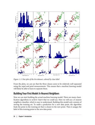
Figure 1-3 is a pair plot of the features in the training set. The data points are colored
according to the species the iris belongs to. To create the plot, we first convert the
NumPy array into a pandas DataFrame. pandas has a function to create pair plots
called scatter_matrix. The diagonal of this matrix is filled with histograms of each
feature:
In[24]:
# create dataframe from data in X_train
# label the columns using the strings in iris_dataset.feature_names
iris_dataframe = pd.DataFrame(X_train, columns=iris_dataset.feature_names)
# create a scatter matrix from the dataframe, color by y_train
grr = pd.scatter_matrix(iris_dataframe, c=y_train, figsize=(15, 15), marker='o',
hist_kwds={'bins': 20}, s=60, alpha=.8, cmap=mglearn.cm3)
A First Application: Classifying Iris Species | 19](https://image.slidesharecdn.com/introductiontomachinelearningwithpythonpdfdrive-230107170822-bfb01dbd/85/Introduction-to-Machine-Learning-with-Python-PDFDrive-com-pdf-33-320.jpg)
![The k in k-nearest neighbors signifies that instead of using only the closest neighbor
to the new data point, we can consider any fixed number k of neighbors in the train‐
ing (for example, the closest three or five neighbors). Then, we can make a prediction
using the majority class among these neighbors. We will go into more detail about
this in Chapter 2; for now, we’ll use only a single neighbor.
All machine learning models in scikit-learn are implemented in their own classes,
which are called Estimator classes. The k-nearest neighbors classification algorithm
is implemented in the KNeighborsClassifier class in the neighbors module. Before
we can use the model, we need to instantiate the class into an object. This is when we
will set any parameters of the model. The most important parameter of KNeighbor
sClassifier is the number of neighbors, which we will set to 1:
In[25]:
from sklearn.neighbors import KNeighborsClassifier
knn = KNeighborsClassifier(n_neighbors=1)
The knn object encapsulates the algorithm that will be used to build the model from
the training data, as well the algorithm to make predictions on new data points. It will
also hold the information that the algorithm has extracted from the training data. In
the case of KNeighborsClassifier, it will just store the training set.
To build the model on the training set, we call the fit method of the knn object,
which takes as arguments the NumPy array X_train containing the training data and
the NumPy array y_train of the corresponding training labels:
In[26]:
knn.fit(X_train, y_train)
Out[26]:
KNeighborsClassifier(algorithm='auto', leaf_size=30, metric='minkowski',
metric_params=None, n_jobs=1, n_neighbors=1, p=2,
weights='uniform')
The fit method returns the knn object itself (and modifies it in place), so we get a
string representation of our classifier. The representation shows us which parameters
were used in creating the model. Nearly all of them are the default values, but you can
also find n_neighbors=1, which is the parameter that we passed. Most models in
scikit-learn have many parameters, but the majority of them are either speed opti‐
mizations or for very special use cases. You don’t have to worry about the other
parameters shown in this representation. Printing a scikit-learn model can yield
very long strings, but don’t be intimidated by these. We will cover all the important
parameters in Chapter 2. In the remainder of this book, we will not show the output
of fit because it doesn’t contain any new information.
A First Application: Classifying Iris Species | 21](https://image.slidesharecdn.com/introductiontomachinelearningwithpythonpdfdrive-230107170822-bfb01dbd/85/Introduction-to-Machine-Learning-with-Python-PDFDrive-com-pdf-35-320.jpg)
![Making Predictions
We can now make predictions using this model on new data for which we might not
know the correct labels. Imagine we found an iris in the wild with a sepal length of
5 cm, a sepal width of 2.9 cm, a petal length of 1 cm, and a petal width of 0.2 cm.
What species of iris would this be? We can put this data into a NumPy array, again by
calculating the shape—that is, the number of samples (1) multiplied by the number of
features (4):
In[27]:
X_new = np.array([[5, 2.9, 1, 0.2]])
print("X_new.shape: {}".format(X_new.shape))
Out[27]:
X_new.shape: (1, 4)
Note that we made the measurements of this single flower into a row in a two-
dimensional NumPy array, as scikit-learn always expects two-dimensional arrays
for the data.
To make a prediction, we call the predict method of the knn object:
In[28]:
prediction = knn.predict(X_new)
print("Prediction: {}".format(prediction))
print("Predicted target name: {}".format(
iris_dataset['target_names'][prediction]))
Out[28]:
Prediction: [0]
Predicted target name: ['setosa']
Our model predicts that this new iris belongs to the class 0, meaning its species is
setosa. But how do we know whether we can trust our model? We don’t know the cor‐
rect species of this sample, which is the whole point of building the model!
Evaluating the Model
This is where the test set that we created earlier comes in. This data was not used to
build the model, but we do know what the correct species is for each iris in the test
set.
Therefore, we can make a prediction for each iris in the test data and compare it
against its label (the known species). We can measure how well the model works by
computing the accuracy, which is the fraction of flowers for which the right species
was predicted:
22 | Chapter 1: Introduction](https://image.slidesharecdn.com/introductiontomachinelearningwithpythonpdfdrive-230107170822-bfb01dbd/85/Introduction-to-Machine-Learning-with-Python-PDFDrive-com-pdf-36-320.jpg)
![In[29]:
y_pred = knn.predict(X_test)
print("Test set predictions:n {}".format(y_pred))
Out[29]:
Test set predictions:
[2 1 0 2 0 2 0 1 1 1 2 1 1 1 1 0 1 1 0 0 2 1 0 0 2 0 0 1 1 0 2 1 0 2 2 1 0 2]
In[30]:
print("Test set score: {:.2f}".format(np.mean(y_pred == y_test)))
Out[30]:
Test set score: 0.97
We can also use the score method of the knn object, which will compute the test set
accuracy for us:
In[31]:
print("Test set score: {:.2f}".format(knn.score(X_test, y_test)))
Out[31]:
Test set score: 0.97
For this model, the test set accuracy is about 0.97, which means we made the right
prediction for 97% of the irises in the test set. Under some mathematical assump‐
tions, this means that we can expect our model to be correct 97% of the time for new
irises. For our hobby botanist application, this high level of accuracy means that our
model may be trustworthy enough to use. In later chapters we will discuss how we
can improve performance, and what caveats there are in tuning a model.
Summary and Outlook
Let’s summarize what we learned in this chapter. We started with a brief introduction
to machine learning and its applications, then discussed the distinction between
supervised and unsupervised learning and gave an overview of the tools we’ll be
using in this book. Then, we formulated the task of predicting which species of iris a
particular flower belongs to by using physical measurements of the flower. We used a
dataset of measurements that was annotated by an expert with the correct species to
build our model, making this a supervised learning task. There were three possible
species, setosa, versicolor, or virginica, which made the task a three-class classification
problem. The possible species are called classes in the classification problem, and the
species of a single iris is called its label.
The Iris dataset consists of two NumPy arrays: one containing the data, which is
referred to as X in scikit-learn, and one containing the correct or desired outputs,
Summary and Outlook | 23](https://image.slidesharecdn.com/introductiontomachinelearningwithpythonpdfdrive-230107170822-bfb01dbd/85/Introduction-to-Machine-Learning-with-Python-PDFDrive-com-pdf-37-320.jpg)
![which is called y. The array X is a two-dimensional array of features, with one row per
data point and one column per feature. The array y is a one-dimensional array, which
here contains one class label, an integer ranging from 0 to 2, for each of the samples.
We split our dataset into a training set, to build our model, and a test set, to evaluate
how well our model will generalize to new, previously unseen data.
We chose the k-nearest neighbors classification algorithm, which makes predictions
for a new data point by considering its closest neighbor(s) in the training set. This is
implemented in the KNeighborsClassifier class, which contains the algorithm that
builds the model as well as the algorithm that makes a prediction using the model.
We instantiated the class, setting parameters. Then we built the model by calling the
fit method, passing the training data (X_train) and training outputs (y_train) as
parameters. We evaluated the model using the score method, which computes the
accuracy of the model. We applied the score method to the test set data and the test
set labels and found that our model is about 97% accurate, meaning it is correct 97%
of the time on the test set.
This gave us the confidence to apply the model to new data (in our example, new
flower measurements) and trust that the model will be correct about 97% of the time.
Here is a summary of the code needed for the whole training and evaluation
procedure:
In[32]:
X_train, X_test, y_train, y_test = train_test_split(
iris_dataset['data'], iris_dataset['target'], random_state=0)
knn = KNeighborsClassifier(n_neighbors=1)
knn.fit(X_train, y_train)
print("Test set score: {:.2f}".format(knn.score(X_test, y_test)))
Out[32]:
Test set score: 0.97
This snippet contains the core code for applying any machine learning algorithm
using scikit-learn. The fit, predict, and score methods are the common inter‐
face to supervised models in scikit-learn, and with the concepts introduced in this
chapter, you can apply these models to many machine learning tasks. In the next
chapter, we will go into more depth about the different kinds of supervised models in
scikit-learn and how to apply them successfully.
24 | Chapter 1: Introduction](https://image.slidesharecdn.com/introductiontomachinelearningwithpythonpdfdrive-230107170822-bfb01dbd/85/Introduction-to-Machine-Learning-with-Python-PDFDrive-com-pdf-38-320.jpg)

![4 Discussing all of them is beyond the scope of the book, and we refer you to the scikit-learn documentation
for more details.
view of how each algorithm builds a model. We will examine the strengths and weak‐
nesses of each algorithm, and what kind of data they can best be applied to. We will
also explain the meaning of the most important parameters and options.4
Many algo‐
rithms have a classification and a regression variant, and we will describe both.
It is not necessary to read through the descriptions of each algorithm in detail, but
understanding the models will give you a better feeling for the different ways
machine learning algorithms can work. This chapter can also be used as a reference
guide, and you can come back to it when you are unsure about the workings of any of
the algorithms.
Some Sample Datasets
We will use several datasets to illustrate the different algorithms. Some of the datasets
will be small and synthetic (meaning made-up), designed to highlight particular
aspects of the algorithms. Other datasets will be large, real-world examples.
An example of a synthetic two-class classification dataset is the forge dataset, which
has two features. The following code creates a scatter plot (Figure 2-2) visualizing all
of the data points in this dataset. The plot has the first feature on the x-axis and the
second feature on the y-axis. As is always the case in scatter plots, each data point is
represented as one dot. The color and shape of the dot indicates its class:
In[2]:
# generate dataset
X, y = mglearn.datasets.make_forge()
# plot dataset
mglearn.discrete_scatter(X[:, 0], X[:, 1], y)
plt.legend(["Class 0", "Class 1"], loc=4)
plt.xlabel("First feature")
plt.ylabel("Second feature")
print("X.shape: {}".format(X.shape))
Out[2]:
X.shape: (26, 2)
30 | Chapter 2: Supervised Learning](https://image.slidesharecdn.com/introductiontomachinelearningwithpythonpdfdrive-230107170822-bfb01dbd/85/Introduction-to-Machine-Learning-with-Python-PDFDrive-com-pdf-44-320.jpg)
![Figure 2-2. Scatter plot of the forge dataset
As you can see from X.shape, this dataset consists of 26 data points, with 2 features.
To illustrate regression algorithms, we will use the synthetic wave dataset. The wave
dataset has a single input feature and a continuous target variable (or response) that
we want to model. The plot created here (Figure 2-3) shows the single feature on the
x-axis and the regression target (the output) on the y-axis:
In[3]:
X, y = mglearn.datasets.make_wave(n_samples=40)
plt.plot(X, y, 'o')
plt.ylim(-3, 3)
plt.xlabel("Feature")
plt.ylabel("Target")
Supervised Machine Learning Algorithms | 31](https://image.slidesharecdn.com/introductiontomachinelearningwithpythonpdfdrive-230107170822-bfb01dbd/85/Introduction-to-Machine-Learning-with-Python-PDFDrive-com-pdf-45-320.jpg)
![Figure 2-3. Plot of the wave dataset, with the x-axis showing the feature and the y-axis
showing the regression target
We are using these very simple, low-dimensional datasets because we can easily visu‐
alize them—a printed page has two dimensions, so data with more than two features
is hard to show. Any intuition derived from datasets with few features (also called
low-dimensional datasets) might not hold in datasets with many features (high-
dimensional datasets). As long as you keep that in mind, inspecting algorithms on
low-dimensional datasets can be very instructive.
We will complement these small synthetic datasets with two real-world datasets that
are included in scikit-learn. One is the Wisconsin Breast Cancer dataset (cancer,
for short), which records clinical measurements of breast cancer tumors. Each tumor
is labeled as “benign” (for harmless tumors) or “malignant” (for cancerous tumors),
and the task is to learn to predict whether a tumor is malignant based on the meas‐
urements of the tissue.
The data can be loaded using the load_breast_cancer function from scikit-learn:
In[4]:
from sklearn.datasets import load_breast_cancer
cancer = load_breast_cancer()
print("cancer.keys(): n{}".format(cancer.keys()))
32 | Chapter 2: Supervised Learning](https://image.slidesharecdn.com/introductiontomachinelearningwithpythonpdfdrive-230107170822-bfb01dbd/85/Introduction-to-Machine-Learning-with-Python-PDFDrive-com-pdf-46-320.jpg)
![Out[4]:
cancer.keys():
dict_keys(['feature_names', 'data', 'DESCR', 'target', 'target_names'])
Datasets that are included in scikit-learn are usually stored as
Bunch objects, which contain some information about the dataset
as well as the actual data. All you need to know about Bunch objects
is that they behave like dictionaries, with the added benefit that you
can access values using a dot (as in bunch.key instead of
bunch['key']).
The dataset consists of 569 data points, with 30 features each:
In[5]:
print("Shape of cancer data: {}".format(cancer.data.shape))
Out[5]:
Shape of cancer data: (569, 30)
Of these 569 data points, 212 are labeled as malignant and 357 as benign:
In[6]:
print("Sample counts per class:n{}".format(
{n: v for n, v in zip(cancer.target_names, np.bincount(cancer.target))}))
Out[6]:
Sample counts per class:
{'benign': 357, 'malignant': 212}
To get a description of the semantic meaning of each feature, we can have a look at
the feature_names attribute:
In[7]:
print("Feature names:n{}".format(cancer.feature_names))
Out[7]:
Feature names:
['mean radius' 'mean texture' 'mean perimeter' 'mean area'
'mean smoothness' 'mean compactness' 'mean concavity'
'mean concave points' 'mean symmetry' 'mean fractal dimension'
'radius error' 'texture error' 'perimeter error' 'area error'
'smoothness error' 'compactness error' 'concavity error'
'concave points error' 'symmetry error' 'fractal dimension error'
'worst radius' 'worst texture' 'worst perimeter' 'worst area'
'worst smoothness' 'worst compactness' 'worst concavity'
'worst concave points' 'worst symmetry' 'worst fractal dimension']
Supervised Machine Learning Algorithms | 33](https://image.slidesharecdn.com/introductiontomachinelearningwithpythonpdfdrive-230107170822-bfb01dbd/85/Introduction-to-Machine-Learning-with-Python-PDFDrive-com-pdf-47-320.jpg)
![5 This is called the binomial coefficient, which is the number of combinations of k elements that can be selected
from a set of n elements. Often this is written as
n
k
and spoken as “n choose k”—in this case, “13 choose 2.”
You can find out more about the data by reading cancer.DESCR if you are interested.
We will also be using a real-world regression dataset, the Boston Housing dataset.
The task associated with this dataset is to predict the median value of homes in sev‐
eral Boston neighborhoods in the 1970s, using information such as crime rate, prox‐
imity to the Charles River, highway accessibility, and so on. The dataset contains 506
data points, described by 13 features:
In[8]:
from sklearn.datasets import load_boston
boston = load_boston()
print("Data shape: {}".format(boston.data.shape))
Out[8]:
Data shape: (506, 13)
Again, you can get more information about the dataset by reading the DESCR attribute
of boston. For our purposes here, we will actually expand this dataset by not only
considering these 13 measurements as input features, but also looking at all products
(also called interactions) between features. In other words, we will not only consider
crime rate and highway accessibility as features, but also the product of crime rate
and highway accessibility. Including derived feature like these is called feature engi‐
neering, which we will discuss in more detail in Chapter 4. This derived dataset can be
loaded using the load_extended_boston function:
In[9]:
X, y = mglearn.datasets.load_extended_boston()
print("X.shape: {}".format(X.shape))
Out[9]:
X.shape: (506, 104)
The resulting 104 features are the 13 original features together with the 91 possible
combinations of two features within those 13.5
We will use these datasets to explain and illustrate the properties of the different
machine learning algorithms. But for now, let’s get to the algorithms themselves.
First, we will revisit the k-nearest neighbors (k-NN) algorithm that we saw in the pre‐
vious chapter.
34 | Chapter 2: Supervised Learning](https://image.slidesharecdn.com/introductiontomachinelearningwithpythonpdfdrive-230107170822-bfb01dbd/85/Introduction-to-Machine-Learning-with-Python-PDFDrive-com-pdf-48-320.jpg)
![k-Nearest Neighbors
The k-NN algorithm is arguably the simplest machine learning algorithm. Building
the model consists only of storing the training dataset. To make a prediction for a
new data point, the algorithm finds the closest data points in the training dataset—its
“nearest neighbors.”
k-Neighbors classification
In its simplest version, the k-NN algorithm only considers exactly one nearest neigh‐
bor, which is the closest training data point to the point we want to make a prediction
for. The prediction is then simply the known output for this training point. Figure 2-4
illustrates this for the case of classification on the forge dataset:
In[10]:
mglearn.plots.plot_knn_classification(n_neighbors=1)
Figure 2-4. Predictions made by the one-nearest-neighbor model on the forge dataset
Here, we added three new data points, shown as stars. For each of them, we marked
the closest point in the training set. The prediction of the one-nearest-neighbor algo‐
rithm is the label of that point (shown by the color of the cross).
Supervised Machine Learning Algorithms | 35](https://image.slidesharecdn.com/introductiontomachinelearningwithpythonpdfdrive-230107170822-bfb01dbd/85/Introduction-to-Machine-Learning-with-Python-PDFDrive-com-pdf-49-320.jpg)
![Instead of considering only the closest neighbor, we can also consider an arbitrary
number, k, of neighbors. This is where the name of the k-nearest neighbors algorithm
comes from. When considering more than one neighbor, we use voting to assign a
label. This means that for each test point, we count how many neighbors belong to
class 0 and how many neighbors belong to class 1. We then assign the class that is
more frequent: in other words, the majority class among the k-nearest neighbors. The
following example (Figure 2-5) uses the three closest neighbors:
In[11]:
mglearn.plots.plot_knn_classification(n_neighbors=3)
Figure 2-5. Predictions made by the three-nearest-neighbors model on the forge dataset
Again, the prediction is shown as the color of the cross. You can see that the predic‐
tion for the new data point at the top left is not the same as the prediction when we
used only one neighbor.
While this illustration is for a binary classification problem, this method can be
applied to datasets with any number of classes. For more classes, we count how many
neighbors belong to each class and again predict the most common class.
Now let’s look at how we can apply the k-nearest neighbors algorithm using scikit-
learn. First, we split our data into a training and a test set so we can evaluate general‐
ization performance, as discussed in Chapter 1:
36 | Chapter 2: Supervised Learning](https://image.slidesharecdn.com/introductiontomachinelearningwithpythonpdfdrive-230107170822-bfb01dbd/85/Introduction-to-Machine-Learning-with-Python-PDFDrive-com-pdf-50-320.jpg)
![In[12]:
from sklearn.model_selection import train_test_split
X, y = mglearn.datasets.make_forge()
X_train, X_test, y_train, y_test = train_test_split(X, y, random_state=0)
Next, we import and instantiate the class. This is when we can set parameters, like the
number of neighbors to use. Here, we set it to 3:
In[13]:
from sklearn.neighbors import KNeighborsClassifier
clf = KNeighborsClassifier(n_neighbors=3)
Now, we fit the classifier using the training set. For KNeighborsClassifier this
means storing the dataset, so we can compute neighbors during prediction:
In[14]:
clf.fit(X_train, y_train)
To make predictions on the test data, we call the predict method. For each data point
in the test set, this computes its nearest neighbors in the training set and finds the
most common class among these:
In[15]:
print("Test set predictions: {}".format(clf.predict(X_test)))
Out[15]:
Test set predictions: [1 0 1 0 1 0 0]
To evaluate how well our model generalizes, we can call the score method with the
test data together with the test labels:
In[16]:
print("Test set accuracy: {:.2f}".format(clf.score(X_test, y_test)))
Out[16]:
Test set accuracy: 0.86
We see that our model is about 86% accurate, meaning the model predicted the class
correctly for 86% of the samples in the test dataset.
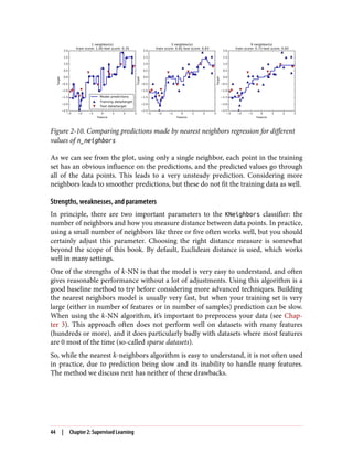
Analyzing KNeighborsClassifier
For two-dimensional datasets, we can also illustrate the prediction for all possible test
points in the xy-plane. We color the plane according to the class that would be
assigned to a point in this region. This lets us view the decision boundary, which is the
divide between where the algorithm assigns class 0 versus where it assigns class 1.
Supervised Machine Learning Algorithms | 37](https://image.slidesharecdn.com/introductiontomachinelearningwithpythonpdfdrive-230107170822-bfb01dbd/85/Introduction-to-Machine-Learning-with-Python-PDFDrive-com-pdf-51-320.jpg)
![The following code produces the visualizations of the decision boundaries for one,
three, and nine neighbors shown in Figure 2-6:
In[17]:
fig, axes = plt.subplots(1, 3, figsize=(10, 3))
for n_neighbors, ax in zip([1, 3, 9], axes):
# the fit method returns the object self, so we can instantiate
# and fit in one line
clf = KNeighborsClassifier(n_neighbors=n_neighbors).fit(X, y)
mglearn.plots.plot_2d_separator(clf, X, fill=True, eps=0.5, ax=ax, alpha=.4)
mglearn.discrete_scatter(X[:, 0], X[:, 1], y, ax=ax)
ax.set_title("{} neighbor(s)".format(n_neighbors))
ax.set_xlabel("feature 0")
ax.set_ylabel("feature 1")
axes[0].legend(loc=3)
Figure 2-6. Decision boundaries created by the nearest neighbors model for different val‐
ues of n_neighbors
As you can see on the left in the figure, using a single neighbor results in a decision
boundary that follows the training data closely. Considering more and more neigh‐
bors leads to a smoother decision boundary. A smoother boundary corresponds to a
simpler model. In other words, using few neighbors corresponds to high model com‐
plexity (as shown on the right side of Figure 2-1), and using many neighbors corre‐
sponds to low model complexity (as shown on the left side of Figure 2-1). If you
consider the extreme case where the number of neighbors is the number of all data
points in the training set, each test point would have exactly the same neighbors (all
training points) and all predictions would be the same: the class that is most frequent
in the training set.
Let’s investigate whether we can confirm the connection between model complexity
and generalization that we discussed earlier. We will do this on the real-world Breast
Cancer dataset. We begin by splitting the dataset into a training and a test set. Then
38 | Chapter 2: Supervised Learning](https://image.slidesharecdn.com/introductiontomachinelearningwithpythonpdfdrive-230107170822-bfb01dbd/85/Introduction-to-Machine-Learning-with-Python-PDFDrive-com-pdf-52-320.jpg)
![we evaluate training and test set performance with different numbers of neighbors.
The results are shown in Figure 2-7:
In[18]:
from sklearn.datasets import load_breast_cancer
cancer = load_breast_cancer()
X_train, X_test, y_train, y_test = train_test_split(
cancer.data, cancer.target, stratify=cancer.target, random_state=66)
training_accuracy = []
test_accuracy = []
# try n_neighbors from 1 to 10
neighbors_settings = range(1, 11)
for n_neighbors in neighbors_settings:
# build the model
clf = KNeighborsClassifier(n_neighbors=n_neighbors)
clf.fit(X_train, y_train)
# record training set accuracy
training_accuracy.append(clf.score(X_train, y_train))
# record generalization accuracy
test_accuracy.append(clf.score(X_test, y_test))
plt.plot(neighbors_settings, training_accuracy, label="training accuracy")
plt.plot(neighbors_settings, test_accuracy, label="test accuracy")
plt.ylabel("Accuracy")
plt.xlabel("n_neighbors")
plt.legend()
The plot shows the training and test set accuracy on the y-axis against the setting of
n_neighbors on the x-axis. While real-world plots are rarely very smooth, we can still
recognize some of the characteristics of overfitting and underfitting (note that
because considering fewer neighbors corresponds to a more complex model, the plot
is horizontally flipped relative to the illustration in Figure 2-1). Considering a single
nearest neighbor, the prediction on the training set is perfect. But when more neigh‐
bors are considered, the model becomes simpler and the training accuracy drops. The
test set accuracy for using a single neighbor is lower than when using more neigh‐
bors, indicating that using the single nearest neighbor leads to a model that is too
complex. On the other hand, when considering 10 neighbors, the model is too simple
and performance is even worse. The best performance is somewhere in the middle,
using around six neighbors. Still, it is good to keep the scale of the plot in mind. The
worst performance is around 88% accuracy, which might still be acceptable.
Supervised Machine Learning Algorithms | 39](https://image.slidesharecdn.com/introductiontomachinelearningwithpythonpdfdrive-230107170822-bfb01dbd/85/Introduction-to-Machine-Learning-with-Python-PDFDrive-com-pdf-53-320.jpg)
![Figure 2-7. Comparison of training and test accuracy as a function of n_neighbors
k-neighbors regression
There is also a regression variant of the k-nearest neighbors algorithm. Again, let’s
start by using the single nearest neighbor, this time using the wave dataset. We’ve
added three test data points as green stars on the x-axis. The prediction using a single
neighbor is just the target value of the nearest neighbor. These are shown as blue stars
in Figure 2-8:
In[19]:
mglearn.plots.plot_knn_regression(n_neighbors=1)
40 | Chapter 2: Supervised Learning](https://image.slidesharecdn.com/introductiontomachinelearningwithpythonpdfdrive-230107170822-bfb01dbd/85/Introduction-to-Machine-Learning-with-Python-PDFDrive-com-pdf-54-320.jpg)
![Figure 2-8. Predictions made by one-nearest-neighbor regression on the wave dataset
Again, we can use more than the single closest neighbor for regression. When using
multiple nearest neighbors, the prediction is the average, or mean, of the relevant
neighbors (Figure 2-9):
In[20]:
mglearn.plots.plot_knn_regression(n_neighbors=3)
Supervised Machine Learning Algorithms | 41](https://image.slidesharecdn.com/introductiontomachinelearningwithpythonpdfdrive-230107170822-bfb01dbd/85/Introduction-to-Machine-Learning-with-Python-PDFDrive-com-pdf-55-320.jpg)
![Figure 2-9. Predictions made by three-nearest-neighbors regression on the wave dataset
The k-nearest neighbors algorithm for regression is implemented in the KNeighbors
Regressor class in scikit-learn. It’s used similarly to KNeighborsClassifier:
In[21]:
from sklearn.neighbors import KNeighborsRegressor
X, y = mglearn.datasets.make_wave(n_samples=40)
# split the wave dataset into a training and a test set
X_train, X_test, y_train, y_test = train_test_split(X, y, random_state=0)
# instantiate the model and set the number of neighbors to consider to 3
reg = KNeighborsRegressor(n_neighbors=3)
# fit the model using the training data and training targets
reg.fit(X_train, y_train)
Now we can make predictions on the test set:
In[22]:
print("Test set predictions:n{}".format(reg.predict(X_test)))
42 | Chapter 2: Supervised Learning](https://image.slidesharecdn.com/introductiontomachinelearningwithpythonpdfdrive-230107170822-bfb01dbd/85/Introduction-to-Machine-Learning-with-Python-PDFDrive-com-pdf-56-320.jpg)
![Out[22]:
Test set predictions:
[-0.054 0.357 1.137 -1.894 -1.139 -1.631 0.357 0.912 -0.447 -1.139]
We can also evaluate the model using the score method, which for regressors returns
the R2
score. The R2
score, also known as the coefficient of determination, is a meas‐
ure of goodness of a prediction for a regression model, and yields a score between 0
and 1. A value of 1 corresponds to a perfect prediction, and a value of 0 corresponds
to a constant model that just predicts the mean of the training set responses, y_train:
In[23]:
print("Test set R^2: {:.2f}".format(reg.score(X_test, y_test)))
Out[23]:
Test set R^2: 0.83
Here, the score is 0.83, which indicates a relatively good model fit.
Analyzing KNeighborsRegressor
For our one-dimensional dataset, we can see what the predictions look like for all
possible feature values (Figure 2-10). To do this, we create a test dataset consisting of
many points on the line:
In[24]:
fig, axes = plt.subplots(1, 3, figsize=(15, 4))
# create 1,000 data points, evenly spaced between -3 and 3
line = np.linspace(-3, 3, 1000).reshape(-1, 1)
for n_neighbors, ax in zip([1, 3, 9], axes):
# make predictions using 1, 3, or 9 neighbors
reg = KNeighborsRegressor(n_neighbors=n_neighbors)
reg.fit(X_train, y_train)
ax.plot(line, reg.predict(line))
ax.plot(X_train, y_train, '^', c=mglearn.cm2(0), markersize=8)
ax.plot(X_test, y_test, 'v', c=mglearn.cm2(1), markersize=8)
ax.set_title(
"{} neighbor(s)n train score: {:.2f} test score: {:.2f}".format(
n_neighbors, reg.score(X_train, y_train),
reg.score(X_test, y_test)))
ax.set_xlabel("Feature")
ax.set_ylabel("Target")
axes[0].legend(["Model predictions", "Training data/target",
"Test data/target"], loc="best")
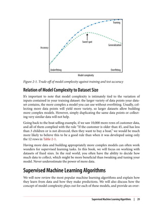
Supervised Machine Learning Algorithms | 43](https://image.slidesharecdn.com/introductiontomachinelearningwithpythonpdfdrive-230107170822-bfb01dbd/85/Introduction-to-Machine-Learning-with-Python-PDFDrive-com-pdf-57-320.jpg)
![Linear Models
Linear models are a class of models that are widely used in practice and have been
studied extensively in the last few decades, with roots going back over a hundred
years. Linear models make a prediction using a linear function of the input features,
which we will explain shortly.
Linear models for regression
For regression, the general prediction formula for a linear model looks as follows:
ŷ = w[0] * x[0] + w[1] * x[1] + ... + w[p] * x[p] + b
Here, x[0] to x[p] denotes the features (in this example, the number of features is p)
of a single data point, w and b are parameters of the model that are learned, and ŷ is
the prediction the model makes. For a dataset with a single feature, this is:
ŷ = w[0] * x[0] + b
which you might remember from high school mathematics as the equation for a line.
Here, w[0] is the slope and b is the y-axis offset. For more features, w contains the
slopes along each feature axis. Alternatively, you can think of the predicted response
as being a weighted sum of the input features, with weights (which can be negative)
given by the entries of w.
Trying to learn the parameters w[0] and b on our one-dimensional wave dataset
might lead to the following line (see Figure 2-11):
In[25]:
mglearn.plots.plot_linear_regression_wave()
Out[25]:
w[0]: 0.393906 b: -0.031804
Supervised Machine Learning Algorithms | 45](https://image.slidesharecdn.com/introductiontomachinelearningwithpythonpdfdrive-230107170822-bfb01dbd/85/Introduction-to-Machine-Learning-with-Python-PDFDrive-com-pdf-59-320.jpg)
![Figure 2-11. Predictions of a linear model on the wave dataset
We added a coordinate cross into the plot to make it easier to understand the line.
Looking at w[0] we see that the slope should be around 0.4, which we can confirm
visually in the plot. The intercept is where the prediction line should cross the y-axis:
this is slightly below zero, which you can also confirm in the image.
Linear models for regression can be characterized as regression models for which the
prediction is a line for a single feature, a plane when using two features, or a hyper‐
plane in higher dimensions (that is, when using more features).
If you compare the predictions made by the straight line with those made by the
KNeighborsRegressor in Figure 2-10, using a straight line to make predictions seems
very restrictive. It looks like all the fine details of the data are lost. In a sense, this is
true. It is a strong (and somewhat unrealistic) assumption that our target y is a linear
46 | Chapter 2: Supervised Learning](https://image.slidesharecdn.com/introductiontomachinelearningwithpythonpdfdrive-230107170822-bfb01dbd/85/Introduction-to-Machine-Learning-with-Python-PDFDrive-com-pdf-60-320.jpg)
![6 This is easy to see if you know some linear algebra.
combination of the features. But looking at one-dimensional data gives a somewhat
skewed perspective. For datasets with many features, linear models can be very pow‐
erful. In particular, if you have more features than training data points, any target y
can be perfectly modeled (on the training set) as a linear function.6
There are many different linear models for regression. The difference between these
models lies in how the model parameters w and b are learned from the training data,
and how model complexity can be controlled. We will now take a look at the most
popular linear models for regression.
Linear regression (aka ordinary least squares)
Linear regression, or ordinary least squares (OLS), is the simplest and most classic lin‐
ear method for regression. Linear regression finds the parameters w and b that mini‐
mize the mean squared error between predictions and the true regression targets, y,
on the training set. The mean squared error is the sum of the squared differences
between the predictions and the true values. Linear regression has no parameters,
which is a benefit, but it also has no way to control model complexity.
Here is the code that produces the model you can see in Figure 2-11:
In[26]:
from sklearn.linear_model import LinearRegression
X, y = mglearn.datasets.make_wave(n_samples=60)
X_train, X_test, y_train, y_test = train_test_split(X, y, random_state=42)
lr = LinearRegression().fit(X_train, y_train)
The “slope” parameters (w), also called weights or coefficients, are stored in the coef_
attribute, while the offset or intercept (b) is stored in the intercept_ attribute:
In[27]:
print("lr.coef_: {}".format(lr.coef_))
print("lr.intercept_: {}".format(lr.intercept_))
Out[27]:
lr.coef_: [ 0.394]
lr.intercept_: -0.031804343026759746
Supervised Machine Learning Algorithms | 47](https://image.slidesharecdn.com/introductiontomachinelearningwithpythonpdfdrive-230107170822-bfb01dbd/85/Introduction-to-Machine-Learning-with-Python-PDFDrive-com-pdf-61-320.jpg)
![You might notice the strange-looking trailing underscore at the end
of coef_ and intercept_. scikit-learn always stores anything
that is derived from the training data in attributes that end with a
trailing underscore. That is to separate them from parameters that
are set by the user.
The intercept_ attribute is always a single float number, while the coef_ attribute is
a NumPy array with one entry per input feature. As we only have a single input fea‐
ture in the wave dataset, lr.coef_ only has a single entry.
Let’s look at the training set and test set performance:
In[28]:
print("Training set score: {:.2f}".format(lr.score(X_train, y_train)))
print("Test set score: {:.2f}".format(lr.score(X_test, y_test)))
Out[28]:
Training set score: 0.67
Test set score: 0.66
An R2
of around 0.66 is not very good, but we can see that the scores on the training
and test sets are very close together. This means we are likely underfitting, not over‐
fitting. For this one-dimensional dataset, there is little danger of overfitting, as the
model is very simple (or restricted). However, with higher-dimensional datasets
(meaning datasets with a large number of features), linear models become more pow‐
erful, and there is a higher chance of overfitting. Let’s take a look at how LinearRe
gression performs on a more complex dataset, like the Boston Housing dataset.
Remember that this dataset has 506 samples and 105 derived features. First, we load
the dataset and split it into a training and a test set. Then we build the linear regres‐
sion model as before:
In[29]:
X, y = mglearn.datasets.load_extended_boston()
X_train, X_test, y_train, y_test = train_test_split(X, y, random_state=0)
lr = LinearRegression().fit(X_train, y_train)
When comparing training set and test set scores, we find that we predict very accu‐
rately on the training set, but the R2
on the test set is much worse:
In[30]:
print("Training set score: {:.2f}".format(lr.score(X_train, y_train)))
print("Test set score: {:.2f}".format(lr.score(X_test, y_test)))
48 | Chapter 2: Supervised Learning](https://image.slidesharecdn.com/introductiontomachinelearningwithpythonpdfdrive-230107170822-bfb01dbd/85/Introduction-to-Machine-Learning-with-Python-PDFDrive-com-pdf-62-320.jpg)
![7 Mathematically, Ridge penalizes the L2 norm of the coefficients, or the Euclidean length of w.
Out[30]:
Training set score: 0.95
Test set score: 0.61
This discrepancy between performance on the training set and the test set is a clear
sign of overfitting, and therefore we should try to find a model that allows us to con‐
trol complexity. One of the most commonly used alternatives to standard linear
regression is ridge regression, which we will look into next.
Ridge regression
Ridge regression is also a linear model for regression, so the formula it uses to make
predictions is the same one used for ordinary least squares. In ridge regression,
though, the coefficients (w) are chosen not only so that they predict well on the train‐
ing data, but also to fit an additional constraint. We also want the magnitude of coef‐
ficients to be as small as possible; in other words, all entries of w should be close to
zero. Intuitively, this means each feature should have as little effect on the outcome as
possible (which translates to having a small slope), while still predicting well. This
constraint is an example of what is called regularization. Regularization means explic‐
itly restricting a model to avoid overfitting. The particular kind used by ridge regres‐
sion is known as L2 regularization.7
Ridge regression is implemented in linear_model.Ridge. Let’s see how well it does
on the extended Boston Housing dataset:
In[31]:
from sklearn.linear_model import Ridge
ridge = Ridge().fit(X_train, y_train)
print("Training set score: {:.2f}".format(ridge.score(X_train, y_train)))
print("Test set score: {:.2f}".format(ridge.score(X_test, y_test)))
Out[31]:
Training set score: 0.89
Test set score: 0.75
As you can see, the training set score of Ridge is lower than for LinearRegression,
while the test set score is higher. This is consistent with our expectation. With linear
regression, we were overfitting our data. Ridge is a more restricted model, so we are
less likely to overfit. A less complex model means worse performance on the training
set, but better generalization. As we are only interested in generalization perfor‐
mance, we should choose the Ridge model over the LinearRegression model.
Supervised Machine Learning Algorithms | 49](https://image.slidesharecdn.com/introductiontomachinelearningwithpythonpdfdrive-230107170822-bfb01dbd/85/Introduction-to-Machine-Learning-with-Python-PDFDrive-com-pdf-63-320.jpg)
![The Ridge model makes a trade-off between the simplicity of the model (near-zero
coefficients) and its performance on the training set. How much importance the
model places on simplicity versus training set performance can be specified by the
user, using the alpha parameter. In the previous example, we used the default param‐
eter alpha=1.0. There is no reason why this will give us the best trade-off, though.
The optimum setting of alpha depends on the particular dataset we are using.
Increasing alpha forces coefficients to move more toward zero, which decreases
training set performance but might help generalization. For example:
In[32]:
ridge10 = Ridge(alpha=10).fit(X_train, y_train)
print("Training set score: {:.2f}".format(ridge10.score(X_train, y_train)))
print("Test set score: {:.2f}".format(ridge10.score(X_test, y_test)))
Out[32]:
Training set score: 0.79
Test set score: 0.64
Decreasing alpha allows the coefficients to be less restricted, meaning we move right
in Figure 2-1. For very small values of alpha, coefficients are barely restricted at all,
and we end up with a model that resembles LinearRegression:
In[33]:
ridge01 = Ridge(alpha=0.1).fit(X_train, y_train)
print("Training set score: {:.2f}".format(ridge01.score(X_train, y_train)))
print("Test set score: {:.2f}".format(ridge01.score(X_test, y_test)))
Out[33]:
Training set score: 0.93
Test set score: 0.77
Here, alpha=0.1 seems to be working well. We could try decreasing alpha even more
to improve generalization. For now, notice how the parameter alpha corresponds to
the model complexity as shown in Figure 2-1. We will discuss methods to properly
select parameters in Chapter 5.
We can also get a more qualitative insight into how the alpha parameter changes the
model by inspecting the coef_ attribute of models with different values of alpha. A
higher alpha means a more restricted model, so we expect the entries of coef_ to
have smaller magnitude for a high value of alpha than for a low value of alpha. This
is confirmed in the plot in Figure 2-12:
50 | Chapter 2: Supervised Learning](https://image.slidesharecdn.com/introductiontomachinelearningwithpythonpdfdrive-230107170822-bfb01dbd/85/Introduction-to-Machine-Learning-with-Python-PDFDrive-com-pdf-64-320.jpg)
![In[34]:
plt.plot(ridge.coef_, 's', label="Ridge alpha=1")
plt.plot(ridge10.coef_, '^', label="Ridge alpha=10")
plt.plot(ridge01.coef_, 'v', label="Ridge alpha=0.1")
plt.plot(lr.coef_, 'o', label="LinearRegression")
plt.xlabel("Coefficient index")
plt.ylabel("Coefficient magnitude")
plt.hlines(0, 0, len(lr.coef_))
plt.ylim(-25, 25)
plt.legend()
Figure 2-12. Comparing coefficient magnitudes for ridge regression with different values
of alpha and linear regression
Here, the x-axis enumerates the entries of coef_: x=0 shows the coefficient associated
with the first feature, x=1 the coefficient associated with the second feature, and so on
up to x=100. The y-axis shows the numeric values of the corresponding values of the
coefficients. The main takeaway here is that for alpha=10, the coefficients are mostly
between around –3 and 3. The coefficients for the Ridge model with alpha=1 are
somewhat larger. The dots corresponding to alpha=0.1 have larger magnitude still,
and many of the dots corresponding to linear regression without any regularization
(which would be alpha=0) are so large they are outside of the chart.
Supervised Machine Learning Algorithms | 51](https://image.slidesharecdn.com/introductiontomachinelearningwithpythonpdfdrive-230107170822-bfb01dbd/85/Introduction-to-Machine-Learning-with-Python-PDFDrive-com-pdf-65-320.jpg)
![Another way to understand the influence of regularization is to fix a value of alpha
but vary the amount of training data available. For Figure 2-13, we subsampled the
Boston Housing dataset and evaluated LinearRegression and Ridge(alpha=1) on
subsets of increasing size (plots that show model performance as a function of dataset
size are called learning curves):
In[35]:
mglearn.plots.plot_ridge_n_samples()
Figure 2-13. Learning curves for ridge regression and linear regression on the Boston
Housing dataset
As one would expect, the training score is higher than the test score for all dataset
sizes, for both ridge and linear regression. Because ridge is regularized, the training
score of ridge is lower than the training score for linear regression across the board.
However, the test score for ridge is better, particularly for small subsets of the data.
For less than 400 data points, linear regression is not able to learn anything. As more
and more data becomes available to the model, both models improve, and linear
regression catches up with ridge in the end. The lesson here is that with enough train‐
ing data, regularization becomes less important, and given enough data, ridge and
52 | Chapter 2: Supervised Learning](https://image.slidesharecdn.com/introductiontomachinelearningwithpythonpdfdrive-230107170822-bfb01dbd/85/Introduction-to-Machine-Learning-with-Python-PDFDrive-com-pdf-66-320.jpg)
![8 The lasso penalizes the L1 norm of the coefficient vector—or in other words, the sum of the absolute values of
the coefficients.
linear regression will have the same performance (the fact that this happens here
when using the full dataset is just by chance). Another interesting aspect of
Figure 2-13 is the decrease in training performance for linear regression. If more data
is added, it becomes harder for a model to overfit, or memorize the data.
Lasso
An alternative to Ridge for regularizing linear regression is Lasso. As with ridge
regression, using the lasso also restricts coefficients to be close to zero, but in a
slightly different way, called L1 regularization.8
The consequence of L1 regularization
is that when using the lasso, some coefficients are exactly zero. This means some fea‐
tures are entirely ignored by the model. This can be seen as a form of automatic fea‐
ture selection. Having some coefficients be exactly zero often makes a model easier to
interpret, and can reveal the most important features of your model.
Let’s apply the lasso to the extended Boston Housing dataset:
In[36]:
from sklearn.linear_model import Lasso
lasso = Lasso().fit(X_train, y_train)
print("Training set score: {:.2f}".format(lasso.score(X_train, y_train)))
print("Test set score: {:.2f}".format(lasso.score(X_test, y_test)))
print("Number of features used: {}".format(np.sum(lasso.coef_ != 0)))
Out[36]:
Training set score: 0.29
Test set score: 0.21
Number of features used: 4
As you can see, Lasso does quite badly, both on the training and the test set. This
indicates that we are underfitting, and we find that it used only 4 of the 105 features.
Similarly to Ridge, the Lasso also has a regularization parameter, alpha, that controls
how strongly coefficients are pushed toward zero. In the previous example, we used
the default of alpha=1.0. To reduce underfitting, let’s try decreasing alpha. When we
do this, we also need to increase the default setting of max_iter (the maximum num‐
ber of iterations to run):
Supervised Machine Learning Algorithms | 53](https://image.slidesharecdn.com/introductiontomachinelearningwithpythonpdfdrive-230107170822-bfb01dbd/85/Introduction-to-Machine-Learning-with-Python-PDFDrive-com-pdf-67-320.jpg)
![In[37]:
# we increase the default setting of "max_iter",
# otherwise the model would warn us that we should increase max_iter.
lasso001 = Lasso(alpha=0.01, max_iter=100000).fit(X_train, y_train)
print("Training set score: {:.2f}".format(lasso001.score(X_train, y_train)))
print("Test set score: {:.2f}".format(lasso001.score(X_test, y_test)))
print("Number of features used: {}".format(np.sum(lasso001.coef_ != 0)))
Out[37]:
Training set score: 0.90
Test set score: 0.77
Number of features used: 33
A lower alpha allowed us to fit a more complex model, which worked better on the
training and test data. The performance is slightly better than using Ridge, and we are
using only 33 of the 105 features. This makes this model potentially easier to under‐
stand.
If we set alpha too low, however, we again remove the effect of regularization and end
up overfitting, with a result similar to LinearRegression:
In[38]:
lasso00001 = Lasso(alpha=0.0001, max_iter=100000).fit(X_train, y_train)
print("Training set score: {:.2f}".format(lasso00001.score(X_train, y_train)))
print("Test set score: {:.2f}".format(lasso00001.score(X_test, y_test)))
print("Number of features used: {}".format(np.sum(lasso00001.coef_ != 0)))
Out[38]:
Training set score: 0.95
Test set score: 0.64
Number of features used: 94
Again, we can plot the coefficients of the different models, similarly to Figure 2-12.
The result is shown in Figure 2-14:
In[39]:
plt.plot(lasso.coef_, 's', label="Lasso alpha=1")
plt.plot(lasso001.coef_, '^', label="Lasso alpha=0.01")
plt.plot(lasso00001.coef_, 'v', label="Lasso alpha=0.0001")
plt.plot(ridge01.coef_, 'o', label="Ridge alpha=0.1")
plt.legend(ncol=2, loc=(0, 1.05))
plt.ylim(-25, 25)
plt.xlabel("Coefficient index")
plt.ylabel("Coefficient magnitude")
54 | Chapter 2: Supervised Learning](https://image.slidesharecdn.com/introductiontomachinelearningwithpythonpdfdrive-230107170822-bfb01dbd/85/Introduction-to-Machine-Learning-with-Python-PDFDrive-com-pdf-68-320.jpg)
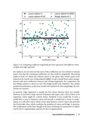
![Linear models for classification
Linear models are also extensively used for classification. Let’s look at binary classifi‐
cation first. In this case, a prediction is made using the following formula:
ŷ = w[0] * x[0] + w[1] * x[1] + ... + w[p] * x[p] + b > 0
The formula looks very similar to the one for linear regression, but instead of just
returning the weighted sum of the features, we threshold the predicted value at zero.
If the function is smaller than zero, we predict the class –1; if it is larger than zero, we
predict the class +1. This prediction rule is common to all linear models for classifica‐
tion. Again, there are many different ways to find the coefficients (w) and the inter‐
cept (b).
For linear models for regression, the output, ŷ, is a linear function of the features: a
line, plane, or hyperplane (in higher dimensions). For linear models for classification,
the decision boundary is a linear function of the input. In other words, a (binary) lin‐
ear classifier is a classifier that separates two classes using a line, a plane, or a hyper‐
plane. We will see examples of that in this section.
There are many algorithms for learning linear models. These algorithms all differ in
the following two ways:
• The way in which they measure how well a particular combination of coefficients
and intercept fits the training data
• If and what kind of regularization they use
Different algorithms choose different ways to measure what “fitting the training set
well” means. For technical mathematical reasons, it is not possible to adjust w and b
to minimize the number of misclassifications the algorithms produce, as one might
hope. For our purposes, and many applications, the different choices for item 1 in the
preceding list (called loss functions) are of little significance.
The two most common linear classification algorithms are logistic regression, imple‐
mented in linear_model.LogisticRegression, and linear support vector machines
(linear SVMs), implemented in svm.LinearSVC (SVC stands for support vector classi‐
fier). Despite its name, LogisticRegression is a classification algorithm and not a
regression algorithm, and it should not be confused with LinearRegression.
We can apply the LogisticRegression and LinearSVC models to the forge dataset,
and visualize the decision boundary as found by the linear models (Figure 2-15):
56 | Chapter 2: Supervised Learning](https://image.slidesharecdn.com/introductiontomachinelearningwithpythonpdfdrive-230107170822-bfb01dbd/85/Introduction-to-Machine-Learning-with-Python-PDFDrive-com-pdf-70-320.jpg)
![In[40]:
from sklearn.linear_model import LogisticRegression
from sklearn.svm import LinearSVC
X, y = mglearn.datasets.make_forge()
fig, axes = plt.subplots(1, 2, figsize=(10, 3))
for model, ax in zip([LinearSVC(), LogisticRegression()], axes):
clf = model.fit(X, y)
mglearn.plots.plot_2d_separator(clf, X, fill=False, eps=0.5,
ax=ax, alpha=.7)
mglearn.discrete_scatter(X[:, 0], X[:, 1], y, ax=ax)
ax.set_title("{}".format(clf.__class__.__name__))
ax.set_xlabel("Feature 0")
ax.set_ylabel("Feature 1")
axes[0].legend()
Figure 2-15. Decision boundaries of a linear SVM and logistic regression on the forge
dataset with the default parameters
In this figure, we have the first feature of the forge dataset on the x-axis and the sec‐
ond feature on the y-axis, as before. We display the decision boundaries found by
LinearSVC and LogisticRegression respectively as straight lines, separating the area
classified as class 1 on the top from the area classified as class 0 on the bottom. In
other words, any new data point that lies above the black line will be classified as class
1 by the respective classifier, while any point that lies below the black line will be clas‐
sified as class 0.
The two models come up with similar decision boundaries. Note that both misclas‐
sify two of the points. By default, both models apply an L2 regularization, in the same
way that Ridge does for regression.
For LogisticRegression and LinearSVC the trade-off parameter that determines the
strength of the regularization is called C, and higher values of C correspond to less
Supervised Machine Learning Algorithms | 57](https://image.slidesharecdn.com/introductiontomachinelearningwithpythonpdfdrive-230107170822-bfb01dbd/85/Introduction-to-Machine-Learning-with-Python-PDFDrive-com-pdf-71-320.jpg)
![regularization. In other words, when you use a high value for the parameter C, Logis
ticRegression and LinearSVC try to fit the training set as best as possible, while with
low values of the parameter C, the models put more emphasis on finding a coefficient
vector (w) that is close to zero.
There is another interesting aspect of how the parameter C acts. Using low values of C
will cause the algorithms to try to adjust to the “majority” of data points, while using
a higher value of C stresses the importance that each individual data point be classi‐
fied correctly. Here is an illustration using LinearSVC (Figure 2-16):
In[41]:
mglearn.plots.plot_linear_svc_regularization()
Figure 2-16. Decision boundaries of a linear SVM on the forge dataset for different
values of C
On the lefthand side, we have a very small C corresponding to a lot of regularization.
Most of the points in class 0 are at the top, and most of the points in class 1 are at the
bottom. The strongly regularized model chooses a relatively horizontal line, misclas‐
sifying two points. In the center plot, C is slightly higher, and the model focuses more
on the two misclassified samples, tilting the decision boundary. Finally, on the right‐
hand side, the very high value of C in the model tilts the decision boundary a lot, now
correctly classifying all points in class 0. One of the points in class 1 is still misclassi‐
fied, as it is not possible to correctly classify all points in this dataset using a straight
line. The model illustrated on the righthand side tries hard to correctly classify all
points, but might not capture the overall layout of the classes well. In other words,
this model is likely overfitting.
Similarly to the case of regression, linear models for classification might seem very
restrictive in low-dimensional spaces, only allowing for decision boundaries that are
straight lines or planes. Again, in high dimensions, linear models for classification
58 | Chapter 2: Supervised Learning](https://image.slidesharecdn.com/introductiontomachinelearningwithpythonpdfdrive-230107170822-bfb01dbd/85/Introduction-to-Machine-Learning-with-Python-PDFDrive-com-pdf-72-320.jpg)
![become very powerful, and guarding against overfitting becomes increasingly impor‐
tant when considering more features.
Let’s analyze LinearLogistic in more detail on the Breast Cancer dataset:
In[42]:
from sklearn.datasets import load_breast_cancer
cancer = load_breast_cancer()
X_train, X_test, y_train, y_test = train_test_split(
cancer.data, cancer.target, stratify=cancer.target, random_state=42)
logreg = LogisticRegression().fit(X_train, y_train)
print("Training set score: {:.3f}".format(logreg.score(X_train, y_train)))
print("Test set score: {:.3f}".format(logreg.score(X_test, y_test)))
Out[42]:
Training set score: 0.953
Test set score: 0.958
The default value of C=1 provides quite good performance, with 95% accuracy on
both the training and the test set. But as training and test set performance are very
close, it is likely that we are underfitting. Let’s try to increase C to fit a more flexible
model:
In[43]:
logreg100 = LogisticRegression(C=100).fit(X_train, y_train)
print("Training set score: {:.3f}".format(logreg100.score(X_train, y_train)))
print("Test set score: {:.3f}".format(logreg100.score(X_test, y_test)))
Out[43]:
Training set score: 0.972
Test set score: 0.965
Using C=100 results in higher training set accuracy, and also a slightly increased test
set accuracy, confirming our intuition that a more complex model should perform
better.
We can also investigate what happens if we use an even more regularized model than
the default of C=1, by setting C=0.01:
In[44]:
logreg001 = LogisticRegression(C=0.01).fit(X_train, y_train)
print("Training set score: {:.3f}".format(logreg001.score(X_train, y_train)))
print("Test set score: {:.3f}".format(logreg001.score(X_test, y_test)))
Out[44]:
Training set score: 0.934
Test set score: 0.930
Supervised Machine Learning Algorithms | 59](https://image.slidesharecdn.com/introductiontomachinelearningwithpythonpdfdrive-230107170822-bfb01dbd/85/Introduction-to-Machine-Learning-with-Python-PDFDrive-com-pdf-73-320.jpg)
![As expected, when moving more to the left along the scale shown in Figure 2-1 from
an already underfit model, both training and test set accuracy decrease relative to the
default parameters.
Finally, let’s look at the coefficients learned by the models with the three different set‐
tings of the regularization parameter C (Figure 2-17):
In[45]:
plt.plot(logreg.coef_.T, 'o', label="C=1")
plt.plot(logreg100.coef_.T, '^', label="C=100")
plt.plot(logreg001.coef_.T, 'v', label="C=0.001")
plt.xticks(range(cancer.data.shape[1]), cancer.feature_names, rotation=90)
plt.hlines(0, 0, cancer.data.shape[1])
plt.ylim(-5, 5)
plt.xlabel("Coefficient index")
plt.ylabel("Coefficient magnitude")
plt.legend()
As LogisticRegression applies an L2 regularization by default,
the result looks similar to that produced by Ridge in Figure 2-12.
Stronger regularization pushes coefficients more and more toward
zero, though coefficients never become exactly zero. Inspecting the
plot more closely, we can also see an interesting effect in the third
coefficient, for “mean perimeter.” For C=100 and C=1, the coefficient
is negative, while for C=0.001, the coefficient is positive, with a
magnitude that is even larger than for C=1. Interpreting a model
like this, one might think the coefficient tells us which class a fea‐
ture is associated with. For example, one might think that a high
“texture error” feature is related to a sample being “malignant.”
However, the change of sign in the coefficient for “mean perimeter”
means that depending on which model we look at, a high “mean
perimeter” could be taken as being either indicative of “benign” or
indicative of “malignant.” This illustrates that interpretations of
coefficients of linear models should always be taken with a grain of
salt.
60 | Chapter 2: Supervised Learning](https://image.slidesharecdn.com/introductiontomachinelearningwithpythonpdfdrive-230107170822-bfb01dbd/85/Introduction-to-Machine-Learning-with-Python-PDFDrive-com-pdf-74-320.jpg)
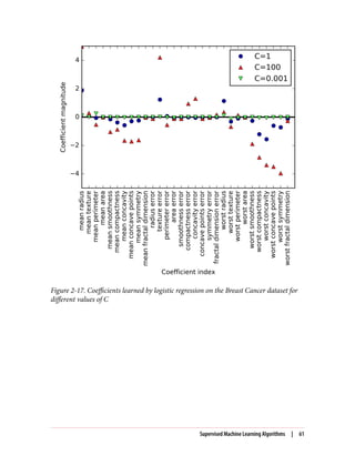
![If we desire a more interpretable model, using L1 regularization might help, as it lim‐
its the model to using only a few features. Here is the coefficient plot and classifica‐
tion accuracies for L1 regularization (Figure 2-18):
In[46]:
for C, marker in zip([0.001, 1, 100], ['o', '^', 'v']):
lr_l1 = LogisticRegression(C=C, penalty="l1").fit(X_train, y_train)
print("Training accuracy of l1 logreg with C={:.3f}: {:.2f}".format(
C, lr_l1.score(X_train, y_train)))
print("Test accuracy of l1 logreg with C={:.3f}: {:.2f}".format(
C, lr_l1.score(X_test, y_test)))
plt.plot(lr_l1.coef_.T, marker, label="C={:.3f}".format(C))
plt.xticks(range(cancer.data.shape[1]), cancer.feature_names, rotation=90)
plt.hlines(0, 0, cancer.data.shape[1])
plt.xlabel("Coefficient index")
plt.ylabel("Coefficient magnitude")
plt.ylim(-5, 5)
plt.legend(loc=3)
Out[46]:
Training accuracy of l1 logreg with C=0.001: 0.91
Test accuracy of l1 logreg with C=0.001: 0.92
Training accuracy of l1 logreg with C=1.000: 0.96
Test accuracy of l1 logreg with C=1.000: 0.96
Training accuracy of l1 logreg with C=100.000: 0.99
Test accuracy of l1 logreg with C=100.000: 0.98
As you can see, there are many parallels between linear models for binary classifica‐
tion and linear models for regression. As in regression, the main difference between
the models is the penalty parameter, which influences the regularization and
whether the model will use all available features or select only a subset.
62 | Chapter 2: Supervised Learning](https://image.slidesharecdn.com/introductiontomachinelearningwithpythonpdfdrive-230107170822-bfb01dbd/85/Introduction-to-Machine-Learning-with-Python-PDFDrive-com-pdf-76-320.jpg)
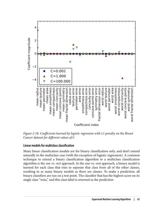
![Having one binary classifier per class results in having one vector of coefficients (w)
and one intercept (b) for each class. The class for which the result of the classification
confidence formula given here is highest is the assigned class label:
w[0] * x[0] + w[1] * x[1] + ... + w[p] * x[p] + b
The mathematics behind multiclass logistic regression differ somewhat from the one-
vs.-rest approach, but they also result in one coefficient vector and intercept per class,
and the same method of making a prediction is applied.
Let’s apply the one-vs.-rest method to a simple three-class classification dataset. We
use a two-dimensional dataset, where each class is given by data sampled from a
Gaussian distribution (see Figure 2-19):
In[47]:
from sklearn.datasets import make_blobs
X, y = make_blobs(random_state=42)
mglearn.discrete_scatter(X[:, 0], X[:, 1], y)
plt.xlabel("Feature 0")
plt.ylabel("Feature 1")
plt.legend(["Class 0", "Class 1", "Class 2"])
Figure 2-19. Two-dimensional toy dataset containing three classes
64 | Chapter 2: Supervised Learning](https://image.slidesharecdn.com/introductiontomachinelearningwithpythonpdfdrive-230107170822-bfb01dbd/85/Introduction-to-Machine-Learning-with-Python-PDFDrive-com-pdf-78-320.jpg)
![Now, we train a LinearSVC classifier on the dataset:
In[48]:
linear_svm = LinearSVC().fit(X, y)
print("Coefficient shape: ", linear_svm.coef_.shape)
print("Intercept shape: ", linear_svm.intercept_.shape)
Out[48]:
Coefficient shape: (3, 2)
Intercept shape: (3,)
We see that the shape of the coef_ is (3, 2), meaning that each row of coef_ con‐
tains the coefficient vector for one of the three classes and each column holds the
coefficient value for a specific feature (there are two in this dataset). The intercept_
is now a one-dimensional array, storing the intercepts for each class.
Let’s visualize the lines given by the three binary classifiers (Figure 2-20):
In[49]:
mglearn.discrete_scatter(X[:, 0], X[:, 1], y)
line = np.linspace(-15, 15)
for coef, intercept, color in zip(linear_svm.coef_, linear_svm.intercept_,
['b', 'r', 'g']):
plt.plot(line, -(line * coef[0] + intercept) / coef[1], c=color)
plt.ylim(-10, 15)
plt.xlim(-10, 8)
plt.xlabel("Feature 0")
plt.ylabel("Feature 1")
plt.legend(['Class 0', 'Class 1', 'Class 2', 'Line class 0', 'Line class 1',
'Line class 2'], loc=(1.01, 0.3))
You can see that all the points belonging to class 0 in the training data are above the
line corresponding to class 0, which means they are on the “class 0” side of this binary
classifier. The points in class 0 are above the line corresponding to class 2, which
means they are classified as “rest” by the binary classifier for class 2. The points
belonging to class 0 are to the left of the line corresponding to class 1, which means
the binary classifier for class 1 also classifies them as “rest.” Therefore, any point in
this area will be classified as class 0 by the final classifier (the result of the classifica‐
tion confidence formula for classifier 0 is greater than zero, while it is smaller than
zero for the other two classes).
But what about the triangle in the middle of the plot? All three binary classifiers clas‐
sify points there as “rest.” Which class would a point there be assigned to? The answer
is the one with the highest value for the classification formula: the class of the closest
line.
Supervised Machine Learning Algorithms | 65](https://image.slidesharecdn.com/introductiontomachinelearningwithpythonpdfdrive-230107170822-bfb01dbd/85/Introduction-to-Machine-Learning-with-Python-PDFDrive-com-pdf-79-320.jpg)
![Figure 2-20. Decision boundaries learned by the three one-vs.-rest classifiers
The following example (Figure 2-21) shows the predictions for all regions of the 2D
space:
In[50]:
mglearn.plots.plot_2d_classification(linear_svm, X, fill=True, alpha=.7)
mglearn.discrete_scatter(X[:, 0], X[:, 1], y)
line = np.linspace(-15, 15)
for coef, intercept, color in zip(linear_svm.coef_, linear_svm.intercept_,
['b', 'r', 'g']):
plt.plot(line, -(line * coef[0] + intercept) / coef[1], c=color)
plt.legend(['Class 0', 'Class 1', 'Class 2', 'Line class 0', 'Line class 1',
'Line class 2'], loc=(1.01, 0.3))
plt.xlabel("Feature 0")
plt.ylabel("Feature 1")
66 | Chapter 2: Supervised Learning](https://image.slidesharecdn.com/introductiontomachinelearningwithpythonpdfdrive-230107170822-bfb01dbd/85/Introduction-to-Machine-Learning-with-Python-PDFDrive-com-pdf-80-320.jpg)
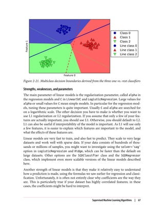
![Linear models often perform well when the number of features is large compared to
the number of samples. They are also often used on very large datasets, simply
because it’s not feasible to train other models. However, in lower-dimensional spaces,
other models might yield better generalization performance. We will look at some
examples in which linear models fail in “Kernelized Support Vector Machines” on
page 92.
Method Chaining
The fit method of all scikit-learn models returns self. This allows you to write
code like the following, which we’ve already used extensively in this chapter:
In[51]:
# instantiate model and fit it in one line
logreg = LogisticRegression().fit(X_train, y_train)
Here, we used the return value of fit (which is self) to assign the trained model to
the variable logreg. This concatenation of method calls (here __init__ and then fit)
is known as method chaining. Another common application of method chaining in
scikit-learn is to fit and predict in one line:
In[52]:
logreg = LogisticRegression()
y_pred = logreg.fit(X_train, y_train).predict(X_test)
Finally, you can even do model instantiation, fitting, and predicting in one line:
In[53]:
y_pred = LogisticRegression().fit(X_train, y_train).predict(X_test)
This very short variant is not ideal, though. A lot is happening in a single line, which
might make the code hard to read. Additionally, the fitted logistic regression model
isn’t stored in any variable, so we can’t inspect it or use it to predict on any other data.
Naive Bayes Classifiers
Naive Bayes classifiers are a family of classifiers that are quite similar to the linear
models discussed in the previous section. However, they tend to be even faster in
training. The price paid for this efficiency is that naive Bayes models often provide
generalization performance that is slightly worse than that of linear classifiers like
LogisticRegression and LinearSVC.
The reason that naive Bayes models are so efficient is that they learn parameters by
looking at each feature individually and collect simple per-class statistics from each
feature. There are three kinds of naive Bayes classifiers implemented in scikit-
68 | Chapter 2: Supervised Learning](https://image.slidesharecdn.com/introductiontomachinelearningwithpythonpdfdrive-230107170822-bfb01dbd/85/Introduction-to-Machine-Learning-with-Python-PDFDrive-com-pdf-82-320.jpg)
![learn: GaussianNB, BernoulliNB, and MultinomialNB. GaussianNB can be applied to
any continuous data, while BernoulliNB assumes binary data and MultinomialNB
assumes count data (that is, that each feature represents an integer count of some‐
thing, like how often a word appears in a sentence). BernoulliNB and MultinomialNB
are mostly used in text data classification.
The BernoulliNB classifier counts how often every feature of each class is not zero.
This is most easily understood with an example:
In[54]:
X = np.array([[0, 1, 0, 1],
[1, 0, 1, 1],
[0, 0, 0, 1],
[1, 0, 1, 0]])
y = np.array([0, 1, 0, 1])
Here, we have four data points, with four binary features each. There are two classes,
0 and 1. For class 0 (the first and third data points), the first feature is zero two times
and nonzero zero times, the second feature is zero one time and nonzero one time,
and so on. These same counts are then calculated for the data points in the second
class. Counting the nonzero entries per class in essence looks like this:
In[55]:
counts = {}
for label in np.unique(y):
# iterate over each class
# count (sum) entries of 1 per feature
counts[label] = X[y == label].sum(axis=0)
print("Feature counts:n{}".format(counts))
Out[55]:
Feature counts:
{0: array([0, 1, 0, 2]), 1: array([2, 0, 2, 1])}
The other two naive Bayes models, MultinomialNB and GaussianNB, are slightly dif‐
ferent in what kinds of statistics they compute. MultinomialNB takes into account the
average value of each feature for each class, while GaussianNB stores the average value
as well as the standard deviation of each feature for each class.
To make a prediction, a data point is compared to the statistics for each of the classes,
and the best matching class is predicted. Interestingly, for both MultinomialNB and
BernoulliNB, this leads to a prediction formula that is of the same form as in the lin‐
ear models (see “Linear models for classification” on page 56). Unfortunately, coef_
for the naive Bayes models has a somewhat different meaning than in the linear mod‐
els, in that coef_ is not the same as w.
Supervised Machine Learning Algorithms | 69](https://image.slidesharecdn.com/introductiontomachinelearningwithpythonpdfdrive-230107170822-bfb01dbd/85/Introduction-to-Machine-Learning-with-Python-PDFDrive-com-pdf-83-320.jpg)
![Strengths, weaknesses, and parameters
MultinomialNB and BernoulliNB have a single parameter, alpha, which controls
model complexity. The way alpha works is that the algorithm adds to the data alpha
many virtual data points that have positive values for all the features. This results in a
“smoothing” of the statistics. A large alpha means more smoothing, resulting in less
complex models. The algorithm’s performance is relatively robust to the setting of
alpha, meaning that setting alpha is not critical for good performance. However,
tuning it usually improves accuracy somewhat.
GaussianNB is mostly used on very high-dimensional data, while the other two var‐
iants of naive Bayes are widely used for sparse count data such as text. MultinomialNB
usually performs better than BinaryNB, particularly on datasets with a relatively large
number of nonzero features (i.e., large documents).
The naive Bayes models share many of the strengths and weaknesses of the linear
models. They are very fast to train and to predict, and the training procedure is easy
to understand. The models work very well with high-dimensional sparse data and are
relatively robust to the parameters. Naive Bayes models are great baseline models and
are often used on very large datasets, where training even a linear model might take
too long.
Decision Trees
Decision trees are widely used models for classification and regression tasks. Essen‐
tially, they learn a hierarchy of if/else questions, leading to a decision.
These questions are similar to the questions you might ask in a game of 20 Questions.
Imagine you want to distinguish between the following four animals: bears, hawks,
penguins, and dolphins. Your goal is to get to the right answer by asking as few if/else
questions as possible. You might start off by asking whether the animal has feathers, a
question that narrows down your possible animals to just two. If the answer is “yes,”
you can ask another question that could help you distinguish between hawks and
penguins. For example, you could ask whether the animal can fly. If the animal
doesn’t have feathers, your possible animal choices are dolphins and bears, and you
will need to ask a question to distinguish between these two animals—for example,
asking whether the animal has fins.
This series of questions can be expressed as a decision tree, as shown in Figure 2-22.
In[56]:
mglearn.plots.plot_animal_tree()
70 | Chapter 2: Supervised Learning](https://image.slidesharecdn.com/introductiontomachinelearningwithpythonpdfdrive-230107170822-bfb01dbd/85/Introduction-to-Machine-Learning-with-Python-PDFDrive-com-pdf-84-320.jpg)
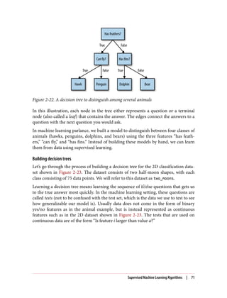
![Figure 2-23. Two-moons dataset on which the decision tree will be built
To build a tree, the algorithm searches over all possible tests and finds the one that is
most informative about the target variable. Figure 2-24 shows the first test that is
picked. Splitting the dataset vertically at x[1]=0.0596 yields the most information; it
best separates the points in class 1 from the points in class 2. The top node, also called
the root, represents the whole dataset, consisting of 75 points belonging to class 0 and
75 points belonging to class 1. The split is done by testing whether x[1] <= 0.0596,
indicated by a black line. If the test is true, a point is assigned to the left node, which
contains 2 points belonging to class 0 and 32 points belonging to class 1. Otherwise
the point is assigned to the right node, which contains 48 points belonging to class 0
and 18 points belonging to class 1. These two nodes correspond to the top and bot‐
tom regions shown in Figure 2-24. Even though the first split did a good job of sepa‐
rating the two classes, the bottom region still contains points belonging to class 0, and
the top region still contains points belonging to class 1. We can build a more accurate
model by repeating the process of looking for the best test in both regions.
Figure 2-25 shows that the most informative next split for the left and the right region
is based on x[0].
72 | Chapter 2: Supervised Learning](https://image.slidesharecdn.com/introductiontomachinelearningwithpythonpdfdrive-230107170822-bfb01dbd/85/Introduction-to-Machine-Learning-with-Python-PDFDrive-com-pdf-86-320.jpg)
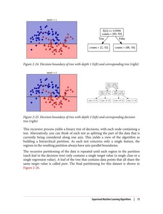
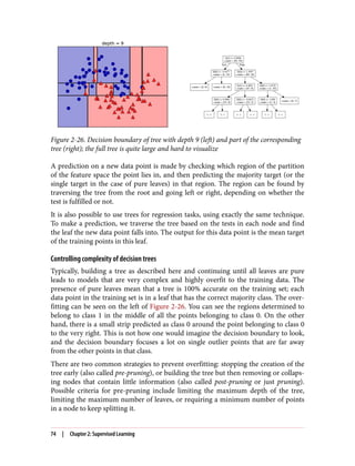
![Decision trees in scikit-learn are implemented in the DecisionTreeRegressor and
DecisionTreeClassifier classes. scikit-learn only implements pre-pruning, not
post-pruning.
Let’s look at the effect of pre-pruning in more detail on the Breast Cancer dataset. As
always, we import the dataset and split it into a training and a test part. Then we build
a model using the default setting of fully developing the tree (growing the tree until
all leaves are pure). We fix the random_state in the tree, which is used for tie-
breaking internally:
In[58]:
from sklearn.tree import DecisionTreeClassifier
cancer = load_breast_cancer()
X_train, X_test, y_train, y_test = train_test_split(
cancer.data, cancer.target, stratify=cancer.target, random_state=42)
tree = DecisionTreeClassifier(random_state=0)
tree.fit(X_train, y_train)
print("Accuracy on training set: {:.3f}".format(tree.score(X_train, y_train)))
print("Accuracy on test set: {:.3f}".format(tree.score(X_test, y_test)))
Out[58]:
Accuracy on training set: 1.000
Accuracy on test set: 0.937
As expected, the accuracy on the training set is 100%—because the leaves are pure,
the tree was grown deep enough that it could perfectly memorize all the labels on the
training data. The test set accuracy is slightly worse than for the linear models we
looked at previously, which had around 95% accuracy.
If we don’t restrict the depth of a decision tree, the tree can become arbitrarily deep
and complex. Unpruned trees are therefore prone to overfitting and not generalizing
well to new data. Now let’s apply pre-pruning to the tree, which will stop developing
the tree before we perfectly fit to the training data. One option is to stop building the
tree after a certain depth has been reached. Here we set max_depth=4, meaning only
four consecutive questions can be asked (cf. Figures 2-24 and 2-26). Limiting the
depth of the tree decreases overfitting. This leads to a lower accuracy on the training
set, but an improvement on the test set:
In[59]:
tree = DecisionTreeClassifier(max_depth=4, random_state=0)
tree.fit(X_train, y_train)
print("Accuracy on training set: {:.3f}".format(tree.score(X_train, y_train)))
print("Accuracy on test set: {:.3f}".format(tree.score(X_test, y_test)))
Supervised Machine Learning Algorithms | 75](https://image.slidesharecdn.com/introductiontomachinelearningwithpythonpdfdrive-230107170822-bfb01dbd/85/Introduction-to-Machine-Learning-with-Python-PDFDrive-com-pdf-89-320.jpg)
![Out[59]:
Accuracy on training set: 0.988
Accuracy on test set: 0.951
Analyzing decision trees
We can visualize the tree using the export_graphviz function from the tree module.
This writes a file in the .dot file format, which is a text file format for storing graphs.
We set an option to color the nodes to reflect the majority class in each node and pass
the class and features names so the tree can be properly labeled:
In[61]:
from sklearn.tree import export_graphviz
export_graphviz(tree, out_file="tree.dot", class_names=["malignant", "benign"],
feature_names=cancer.feature_names, impurity=False, filled=True)
We can read this file and visualize it, as seen in Figure 2-27, using the graphviz mod‐
ule (or you can use any program that can read .dot files):
In[61]:
import graphviz
with open("tree.dot") as f:
dot_graph = f.read()
graphviz.Source(dot_graph)
Figure 2-27. Visualization of the decision tree built on the Breast Cancer dataset
76 | Chapter 2: Supervised Learning](https://image.slidesharecdn.com/introductiontomachinelearningwithpythonpdfdrive-230107170822-bfb01dbd/85/Introduction-to-Machine-Learning-with-Python-PDFDrive-com-pdf-90-320.jpg)
![The visualization of the tree provides a great in-depth view of how the algorithm
makes predictions, and is a good example of a machine learning algorithm that is
easily explained to nonexperts. However, even with a tree of depth four, as seen here,
the tree can become a bit overwhelming. Deeper trees (a depth of 10 is not uncom‐
mon) are even harder to grasp. One method of inspecting the tree that may be helpful
is to find out which path most of the data actually takes. The n_samples shown in
each node in Figure 2-27 gives the number of samples in that node, while value pro‐
vides the number of samples per class. Following the branches to the right, we see
that worst radius <= 16.795 creates a node that contains only 8 benign but 134
malignant samples. The rest of this side of the tree then uses some finer distinctions
to split off these 8 remaining benign samples. Of the 142 samples that went to the
right in the initial split, nearly all of them (132) end up in the leaf to the very right.
Taking a left at the root, for worst radius > 16.795 we end up with 25 malignant
and 259 benign samples. Nearly all of the benign samples end up in the second leaf
from the right, with most of the other leaves containing very few samples.
Feature importance in trees
Instead of looking at the whole tree, which can be taxing, there are some useful prop‐
erties that we can derive to summarize the workings of the tree. The most commonly
used summary is feature importance, which rates how important each feature is for
the decision a tree makes. It is a number between 0 and 1 for each feature, where 0
means “not used at all” and 1 means “perfectly predicts the target.” The feature
importances always sum to 1:
In[62]:
print("Feature importances:n{}".format(tree.feature_importances_))
Out[62]:
Feature importances:
[ 0. 0. 0. 0. 0. 0. 0. 0. 0. 0. 0.01
0.048 0. 0. 0.002 0. 0. 0. 0. 0. 0.727 0.046
0. 0. 0.014 0. 0.018 0.122 0.012 0. ]
We can visualize the feature importances in a way that is similar to the way we visual‐
ize the coefficients in the linear model (Figure 2-28):
In[63]:
def plot_feature_importances_cancer(model):
n_features = cancer.data.shape[1]
plt.barh(range(n_features), model.feature_importances_, align='center')
plt.yticks(np.arange(n_features), cancer.feature_names)
plt.xlabel("Feature importance")
plt.ylabel("Feature")
plot_feature_importances_cancer(tree)
Supervised Machine Learning Algorithms | 77](https://image.slidesharecdn.com/introductiontomachinelearningwithpythonpdfdrive-230107170822-bfb01dbd/85/Introduction-to-Machine-Learning-with-Python-PDFDrive-com-pdf-91-320.jpg)
![Figure 2-28. Feature importances computed from a decision tree learned on the Breast
Cancer dataset
Here we see that the feature used in the top split (“worst radius”) is by far the most
important feature. This confirms our observation in analyzing the tree that the first
level already separates the two classes fairly well.
However, if a feature has a low feature_importance, it doesn’t mean that this feature
is uninformative. It only means that the feature was not picked by the tree, likely
because another feature encodes the same information.
In contrast to the coefficients in linear models, feature importances are always posi‐
tive, and don’t encode which class a feature is indicative of. The feature importances
tell us that “worst radius” is important, but not whether a high radius is indicative of a
sample being benign or malignant. In fact, there might not be such a simple relation‐
ship between features and class, as you can see in the following example (Figures 2-29
and 2-30):
In[64]:
tree = mglearn.plots.plot_tree_not_monotone()
display(tree)
Out[64]:
Feature importances: [ 0. 1.]
78 | Chapter 2: Supervised Learning](https://image.slidesharecdn.com/introductiontomachinelearningwithpythonpdfdrive-230107170822-bfb01dbd/85/Introduction-to-Machine-Learning-with-Python-PDFDrive-com-pdf-92-320.jpg)
![Figure 2-29. A two-dimensional dataset in which the feature on the y-axis has a nonmo‐
notonous relationship with the class label, and the decision boundaries found by a deci‐
sion tree
Figure 2-30. Decision tree learned on the data shown in Figure 2-29
The plot shows a dataset with two features and two classes. Here, all the information
is contained in X[1], and X[0] is not used at all. But the relation between X[1] and
Supervised Machine Learning Algorithms | 79](https://image.slidesharecdn.com/introductiontomachinelearningwithpythonpdfdrive-230107170822-bfb01dbd/85/Introduction-to-Machine-Learning-with-Python-PDFDrive-com-pdf-93-320.jpg)
![the output class is not monotonous, meaning we cannot say “a high value of X[0]
means class 0, and a low value means class 1” (or vice versa).
While we focused our discussion here on decision trees for classification, all that was
said is similarly true for decision trees for regression, as implemented in Decision
TreeRegressor. The usage and analysis of regression trees is very similar to that of
classification trees. There is one particular property of using tree-based models for
regression that we want to point out, though. The DecisionTreeRegressor (and all
other tree-based regression models) is not able to extrapolate, or make predictions
outside of the range of the training data.
Let’s look into this in more detail, using a dataset of historical computer memory
(RAM) prices. Figure 2-31 shows the dataset, with the date on the x-axis and the price
of one megabyte of RAM in that year on the y-axis:
In[65]:
import pandas as pd
ram_prices = pd.read_csv("data/ram_price.csv")
plt.semilogy(ram_prices.date, ram_prices.price)
plt.xlabel("Year")
plt.ylabel("Price in $/Mbyte")
Figure 2-31. Historical development of the price of RAM, plotted on a log scale
80 | Chapter 2: Supervised Learning](https://image.slidesharecdn.com/introductiontomachinelearningwithpythonpdfdrive-230107170822-bfb01dbd/85/Introduction-to-Machine-Learning-with-Python-PDFDrive-com-pdf-94-320.jpg)
![Note the logarithmic scale of the y-axis. When plotting logarithmically, the relation
seems to be quite linear and so should be relatively easy to predict, apart from some
bumps.
We will make a forecast for the years after 2000 using the historical data up to that
point, with the date as our only feature. We will compare two simple models: a
DecisionTreeRegressor and LinearRegression. We rescale the prices using a loga‐
rithm, so that the relationship is relatively linear. This doesn’t make a difference for
the DecisionTreeRegressor, but it makes a big difference for LinearRegression (we
will discuss this in more depth in Chapter 4). After training the models and making
predictions, we apply the exponential map to undo the logarithm transform. We
make predictions on the whole dataset for visualization purposes here, but for a
quantitative evaluation we would only consider the test dataset:
In[66]:
from sklearn.tree import DecisionTreeRegressor
# use historical data to forecast prices after the year 2000
data_train = ram_prices[ram_prices.date < 2000]
data_test = ram_prices[ram_prices.date >= 2000]
# predict prices based on date
X_train = data_train.date[:, np.newaxis]
# we use a log-transform to get a simpler relationship of data to target
y_train = np.log(data_train.price)
tree = DecisionTreeRegressor().fit(X_train, y_train)
linear_reg = LinearRegression().fit(X_train, y_train)
# predict on all data
X_all = ram_prices.date[:, np.newaxis]
pred_tree = tree.predict(X_all)
pred_lr = linear_reg.predict(X_all)
# undo log-transform
price_tree = np.exp(pred_tree)
price_lr = np.exp(pred_lr)
Figure 2-32, created here, compares the predictions of the decision tree and the linear
regression model with the ground truth:
In[67]:
plt.semilogy(data_train.date, data_train.price, label="Training data")
plt.semilogy(data_test.date, data_test.price, label="Test data")
plt.semilogy(ram_prices.date, price_tree, label="Tree prediction")
plt.semilogy(ram_prices.date, price_lr, label="Linear prediction")
plt.legend()
Supervised Machine Learning Algorithms | 81](https://image.slidesharecdn.com/introductiontomachinelearningwithpythonpdfdrive-230107170822-bfb01dbd/85/Introduction-to-Machine-Learning-with-Python-PDFDrive-com-pdf-95-320.jpg)
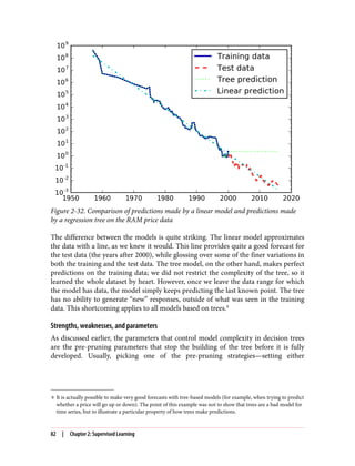
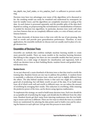
![Building random forests. To build a random forest model, you need to decide on the
number of trees to build (the n_estimators parameter of RandomForestRegressor or
RandomForestClassifier). Let’s say we want to build 10 trees. These trees will be
built completely independently from each other, and the algorithm will make differ‐
ent random choices for each tree to make sure the trees are distinct. To build a tree,
we first take what is called a bootstrap sample of our data. That is, from our n_samples
data points, we repeatedly draw an example randomly with replacement (meaning the
same sample can be picked multiple times), n_samples times. This will create a data‐
set that is as big as the original dataset, but some data points will be missing from it
(approximately one third), and some will be repeated.
To illustrate, let’s say we want to create a bootstrap sample of the list ['a', 'b',
'c', 'd']. A possible bootstrap sample would be ['b', 'd', 'd', 'c']. Another
possible sample would be ['d', 'a', 'd', 'a'].
Next, a decision tree is built based on this newly created dataset. However, the algo‐
rithm we described for the decision tree is slightly modified. Instead of looking for
the best test for each node, in each node the algorithm randomly selects a subset of
the features, and it looks for the best possible test involving one of these features. The
number of features that are selected is controlled by the max_features parameter.
This selection of a subset of features is repeated separately in each node, so that each
node in a tree can make a decision using a different subset of the features.
The bootstrap sampling leads to each decision tree in the random forest being built
on a slightly different dataset. Because of the selection of features in each node, each
split in each tree operates on a different subset of features. Together, these two mech‐
anisms ensure that all the trees in the random forest are different.
A critical parameter in this process is max_features. If we set max_features to n_fea
tures, that means that each split can look at all features in the dataset, and no ran‐
domness will be injected in the feature selection (the randomness due to the
bootstrapping remains, though). If we set max_features to 1, that means that the
splits have no choice at all on which feature to test, and can only search over different
thresholds for the feature that was selected randomly. Therefore, a high max_fea
tures means that the trees in the random forest will be quite similar, and they will be
able to fit the data easily, using the most distinctive features. A low max_features
means that the trees in the random forest will be quite different, and that each tree
might need to be very deep in order to fit the data well.
To make a prediction using the random forest, the algorithm first makes a prediction
for every tree in the forest. For regression, we can average these results to get our final
prediction. For classification, a “soft voting” strategy is used. This means each algo‐
rithm makes a “soft” prediction, providing a probability for each possible output
84 | Chapter 2: Supervised Learning](https://image.slidesharecdn.com/introductiontomachinelearningwithpythonpdfdrive-230107170822-bfb01dbd/85/Introduction-to-Machine-Learning-with-Python-PDFDrive-com-pdf-98-320.jpg)
![label. The probabilities predicted by all the trees are averaged, and the class with the
highest probability is predicted.
Analyzing random forests. Let’s apply a random forest consisting of five trees to the
two_moons dataset we studied earlier:
In[68]:
from sklearn.ensemble import RandomForestClassifier
from sklearn.datasets import make_moons
X, y = make_moons(n_samples=100, noise=0.25, random_state=3)
X_train, X_test, y_train, y_test = train_test_split(X, y, stratify=y,
random_state=42)
forest = RandomForestClassifier(n_estimators=5, random_state=2)
forest.fit(X_train, y_train)
The trees that are built as part of the random forest are stored in the estimator_
attribute. Let’s visualize the decision boundaries learned by each tree, together with
their aggregate prediction as made by the forest (Figure 2-33):
In[69]:
fig, axes = plt.subplots(2, 3, figsize=(20, 10))
for i, (ax, tree) in enumerate(zip(axes.ravel(), forest.estimators_)):
ax.set_title("Tree {}".format(i))
mglearn.plots.plot_tree_partition(X_train, y_train, tree, ax=ax)
mglearn.plots.plot_2d_separator(forest, X_train, fill=True, ax=axes[-1, -1],
alpha=.4)
axes[-1, -1].set_title("Random Forest")
mglearn.discrete_scatter(X_train[:, 0], X_train[:, 1], y_train)
You can clearly see that the decision boundaries learned by the five trees are quite dif‐
ferent. Each of them makes some mistakes, as some of the training points that are
plotted here were not actually included in the training sets of the trees, due to the
bootstrap sampling.
The random forest overfits less than any of the trees individually, and provides a
much more intuitive decision boundary. In any real application, we would use many
more trees (often hundreds or thousands), leading to even smoother boundaries.
Supervised Machine Learning Algorithms | 85](https://image.slidesharecdn.com/introductiontomachinelearningwithpythonpdfdrive-230107170822-bfb01dbd/85/Introduction-to-Machine-Learning-with-Python-PDFDrive-com-pdf-99-320.jpg)
![Figure 2-33. Decision boundaries found by five randomized decision trees and the deci‐
sion boundary obtained by averaging their predicted probabilities
As another example, let’s apply a random forest consisting of 100 trees on the Breast
Cancer dataset:
In[70]:
X_train, X_test, y_train, y_test = train_test_split(
cancer.data, cancer.target, random_state=0)
forest = RandomForestClassifier(n_estimators=100, random_state=0)
forest.fit(X_train, y_train)
print("Accuracy on training set: {:.3f}".format(forest.score(X_train, y_train)))
print("Accuracy on test set: {:.3f}".format(forest.score(X_test, y_test)))
Out[70]:
Accuracy on training set: 1.000
Accuracy on test set: 0.972
The random forest gives us an accuracy of 97%, better than the linear models or a
single decision tree, without tuning any parameters. We could adjust the max_fea
tures setting, or apply pre-pruning as we did for the single decision tree. However,
often the default parameters of the random forest already work quite well.
Similarly to the decision tree, the random forest provides feature importances, which
are computed by aggregating the feature importances over the trees in the forest. Typ‐
ically, the feature importances provided by the random forest are more reliable than
the ones provided by a single tree. Take a look at Figure 2-34.
86 | Chapter 2: Supervised Learning](https://image.slidesharecdn.com/introductiontomachinelearningwithpythonpdfdrive-230107170822-bfb01dbd/85/Introduction-to-Machine-Learning-with-Python-PDFDrive-com-pdf-100-320.jpg)
![In[71]:
plot_feature_importances_cancer(forest)
Figure 2-34. Feature importances computed from a random forest that was fit to the
Breast Cancer dataset
As you can see, the random forest gives nonzero importance to many more features
than the single tree. Similarly to the single decision tree, the random forest also gives
a lot of importance to the “worst radius” feature, but it actually chooses “worst perim‐
eter” to be the most informative feature overall. The randomness in building the ran‐
dom forest forces the algorithm to consider many possible explanations, the result
being that the random forest captures a much broader picture of the data than a sin‐
gle tree.
Strengths, weaknesses, and parameters. Random forests for regression and classifica‐
tion are currently among the most widely used machine learning methods. They are
very powerful, often work well without heavy tuning of the parameters, and don’t
require scaling of the data.
Essentially, random forests share all of the benefits of decision trees, while making up
for some of their deficiencies. One reason to still use decision trees is if you need a
compact representation of the decision-making process. It is basically impossible to
interpret tens or hundreds of trees in detail, and trees in random forests tend to be
deeper than decision trees (because of the use of feature subsets). Therefore, if you
need to summarize the prediction making in a visual way to nonexperts, a single
decision tree might be a better choice. While building random forests on large data‐
sets might be somewhat time consuming, it can be parallelized across multiple CPU
Supervised Machine Learning Algorithms | 87](https://image.slidesharecdn.com/introductiontomachinelearningwithpythonpdfdrive-230107170822-bfb01dbd/85/Introduction-to-Machine-Learning-with-Python-PDFDrive-com-pdf-101-320.jpg)
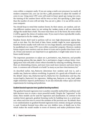
![The main idea behind gradient boosting is to combine many simple models (in this
context known as weak learners), like shallow trees. Each tree can only provide good
predictions on part of the data, and so more and more trees are added to iteratively
improve performance.
Gradient boosted trees are frequently the winning entries in machine learning com‐
petitions, and are widely used in industry. They are generally a bit more sensitive to
parameter settings than random forests, but can provide better accuracy if the param‐
eters are set correctly.
Apart from the pre-pruning and the number of trees in the ensemble, another impor‐
tant parameter of gradient boosting is the learning_rate, which controls how
strongly each tree tries to correct the mistakes of the previous trees. A higher learning
rate means each tree can make stronger corrections, allowing for more complex mod‐
els. Adding more trees to the ensemble, which can be accomplished by increasing
n_estimators, also increases the model complexity, as the model has more chances
to correct mistakes on the training set.
Here is an example of using GradientBoostingClassifier on the Breast Cancer
dataset. By default, 100 trees of maximum depth 3 and a learning rate of 0.1 are used:
In[72]:
from sklearn.ensemble import GradientBoostingClassifier
X_train, X_test, y_train, y_test = train_test_split(
cancer.data, cancer.target, random_state=0)
gbrt = GradientBoostingClassifier(random_state=0)
gbrt.fit(X_train, y_train)
print("Accuracy on training set: {:.3f}".format(gbrt.score(X_train, y_train)))
print("Accuracy on test set: {:.3f}".format(gbrt.score(X_test, y_test)))
Out[72]:
Accuracy on training set: 1.000
Accuracy on test set: 0.958
As the training set accuracy is 100%, we are likely to be overfitting. To reduce overfit‐
ting, we could either apply stronger pre-pruning by limiting the maximum depth or
lower the learning rate:
Supervised Machine Learning Algorithms | 89](https://image.slidesharecdn.com/introductiontomachinelearningwithpythonpdfdrive-230107170822-bfb01dbd/85/Introduction-to-Machine-Learning-with-Python-PDFDrive-com-pdf-103-320.jpg)
![In[73]:
gbrt = GradientBoostingClassifier(random_state=0, max_depth=1)
gbrt.fit(X_train, y_train)
print("Accuracy on training set: {:.3f}".format(gbrt.score(X_train, y_train)))
print("Accuracy on test set: {:.3f}".format(gbrt.score(X_test, y_test)))
Out[73]:
Accuracy on training set: 0.991
Accuracy on test set: 0.972
In[74]:
gbrt = GradientBoostingClassifier(random_state=0, learning_rate=0.01)
gbrt.fit(X_train, y_train)
print("Accuracy on training set: {:.3f}".format(gbrt.score(X_train, y_train)))
print("Accuracy on test set: {:.3f}".format(gbrt.score(X_test, y_test)))
Out[74]:
Accuracy on training set: 0.988
Accuracy on test set: 0.965
Both methods of decreasing the model complexity reduced the training set accuracy,
as expected. In this case, lowering the maximum depth of the trees provided a signifi‐
cant improvement of the model, while lowering the learning rate only increased the
generalization performance slightly.
As for the other decision tree–based models, we can again visualize the feature
importances to get more insight into our model (Figure 2-35). As we used 100 trees, it
is impractical to inspect them all, even if they are all of depth 1:
In[75]:
gbrt = GradientBoostingClassifier(random_state=0, max_depth=1)
gbrt.fit(X_train, y_train)
plot_feature_importances_cancer(gbrt)
90 | Chapter 2: Supervised Learning](https://image.slidesharecdn.com/introductiontomachinelearningwithpythonpdfdrive-230107170822-bfb01dbd/85/Introduction-to-Machine-Learning-with-Python-PDFDrive-com-pdf-104-320.jpg)
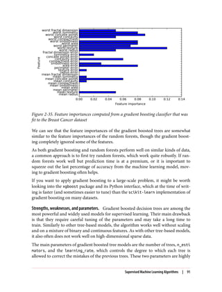
![interconnected, as a lower learning_rate means that more trees are needed to build
a model of similar complexity. In contrast to random forests, where a higher n_esti
mators value is always better, increasing n_estimators in gradient boosting leads to a
more complex model, which may lead to overfitting. A common practice is to fit
n_estimators depending on the time and memory budget, and then search over dif‐
ferent learning_rates.
Another important parameter is max_depth (or alternatively max_leaf_nodes), to
reduce the complexity of each tree. Usually max_depth is set very low for gradient
boosted models, often not deeper than five splits.
Kernelized Support Vector Machines
The next type of supervised model we will discuss is kernelized support vector
machines. We explored the use of linear support vector machines for classification in
“Linear models for classification” on page 56. Kernelized support vector machines
(often just referred to as SVMs) are an extension that allows for more complex mod‐
els that are not defined simply by hyperplanes in the input space. While there are sup‐
port vector machines for classification and regression, we will restrict ourselves to the
classification case, as implemented in SVC. Similar concepts apply to support vector
regression, as implemented in SVR.
The math behind kernelized support vector machines is a bit involved, and is beyond
the scope of this book. You can find the details in Chapter 1 of Hastie, Tibshirani, and
Friedman’s The Elements of Statistical Learning. However, we will try to give you some
sense of the idea behind the method.
Linear models and nonlinear features
As you saw in Figure 2-15, linear models can be quite limiting in low-dimensional
spaces, as lines and hyperplanes have limited flexibility. One way to make a linear
model more flexible is by adding more features—for example, by adding interactions
or polynomials of the input features.
Let’s look at the synthetic dataset we used in “Feature importance in trees” on page 77
(see Figure 2-29):
In[76]:
X, y = make_blobs(centers=4, random_state=8)
y = y % 2
mglearn.discrete_scatter(X[:, 0], X[:, 1], y)
plt.xlabel("Feature 0")
plt.ylabel("Feature 1")
92 | Chapter 2: Supervised Learning](https://image.slidesharecdn.com/introductiontomachinelearningwithpythonpdfdrive-230107170822-bfb01dbd/85/Introduction-to-Machine-Learning-with-Python-PDFDrive-com-pdf-106-320.jpg)
![10 We picked this particular feature to add for illustration purposes. The choice is not particularly important.
Figure 2-36. Two-class classification dataset in which classes are not linearly separable
A linear model for classification can only separate points using a line, and will not be
able to do a very good job on this dataset (see Figure 2-37):
In[77]:
from sklearn.svm import LinearSVC
linear_svm = LinearSVC().fit(X, y)
mglearn.plots.plot_2d_separator(linear_svm, X)
mglearn.discrete_scatter(X[:, 0], X[:, 1], y)
plt.xlabel("Feature 0")
plt.ylabel("Feature 1")
Now let’s expand the set of input features, say by also adding feature1 ** 2, the
square of the second feature, as a new feature. Instead of representing each data point
as a two-dimensional point, (feature0, feature1), we now represent it as a three-
dimensional point, (feature0, feature1, feature1 ** 2).10
This new representa‐
tion is illustrated in Figure 2-38 in a three-dimensional scatter plot:
Supervised Machine Learning Algorithms | 93](https://image.slidesharecdn.com/introductiontomachinelearningwithpythonpdfdrive-230107170822-bfb01dbd/85/Introduction-to-Machine-Learning-with-Python-PDFDrive-com-pdf-107-320.jpg)
![Figure 2-37. Decision boundary found by a linear SVM
In[78]:
# add the squared first feature
X_new = np.hstack([X, X[:, 1:] ** 2])
from mpl_toolkits.mplot3d import Axes3D, axes3d
figure = plt.figure()
# visualize in 3D
ax = Axes3D(figure, elev=-152, azim=-26)
# plot first all the points with y == 0, then all with y == 1
mask = y == 0
ax.scatter(X_new[mask, 0], X_new[mask, 1], X_new[mask, 2], c='b',
cmap=mglearn.cm2, s=60)
ax.scatter(X_new[~mask, 0], X_new[~mask, 1], X_new[~mask, 2], c='r', marker='^',
cmap=mglearn.cm2, s=60)
ax.set_xlabel("feature0")
ax.set_ylabel("feature1")
ax.set_zlabel("feature1 ** 2")
94 | Chapter 2: Supervised Learning](https://image.slidesharecdn.com/introductiontomachinelearningwithpythonpdfdrive-230107170822-bfb01dbd/85/Introduction-to-Machine-Learning-with-Python-PDFDrive-com-pdf-108-320.jpg)
![Figure 2-38. Expansion of the dataset shown in Figure 2-37, created by adding a third
feature derived from feature1
In the new representation of the data, it is now indeed possible to separate the two
classes using a linear model, a plane in three dimensions. We can confirm this by fit‐
ting a linear model to the augmented data (see Figure 2-39):
In[79]:
linear_svm_3d = LinearSVC().fit(X_new, y)
coef, intercept = linear_svm_3d.coef_.ravel(), linear_svm_3d.intercept_
# show linear decision boundary
figure = plt.figure()
ax = Axes3D(figure, elev=-152, azim=-26)
xx = np.linspace(X_new[:, 0].min() - 2, X_new[:, 0].max() + 2, 50)
yy = np.linspace(X_new[:, 1].min() - 2, X_new[:, 1].max() + 2, 50)
XX, YY = np.meshgrid(xx, yy)
ZZ = (coef[0] * XX + coef[1] * YY + intercept) / -coef[2]
ax.plot_surface(XX, YY, ZZ, rstride=8, cstride=8, alpha=0.3)
ax.scatter(X_new[mask, 0], X_new[mask, 1], X_new[mask, 2], c='b',
cmap=mglearn.cm2, s=60)
ax.scatter(X_new[~mask, 0], X_new[~mask, 1], X_new[~mask, 2], c='r', marker='^',
cmap=mglearn.cm2, s=60)
ax.set_xlabel("feature0")
ax.set_ylabel("feature1")
ax.set_zlabel("feature0 ** 2")
Supervised Machine Learning Algorithms | 95](https://image.slidesharecdn.com/introductiontomachinelearningwithpythonpdfdrive-230107170822-bfb01dbd/85/Introduction-to-Machine-Learning-with-Python-PDFDrive-com-pdf-109-320.jpg)
![Figure 2-39. Decision boundary found by a linear SVM on the expanded three-
dimensional dataset
As a function of the original features, the linear SVM model is not actually linear any‐
more. It is not a line, but more of an ellipse, as you can see from the plot created here
(Figure 2-40):
In[80]:
ZZ = YY ** 2
dec = linear_svm_3d.decision_function(np.c_[XX.ravel(), YY.ravel(), ZZ.ravel()])
plt.contourf(XX, YY, dec.reshape(XX.shape), levels=[dec.min(), 0, dec.max()],
cmap=mglearn.cm2, alpha=0.5)
mglearn.discrete_scatter(X[:, 0], X[:, 1], y)
plt.xlabel("Feature 0")
plt.ylabel("Feature 1")
96 | Chapter 2: Supervised Learning](https://image.slidesharecdn.com/introductiontomachinelearningwithpythonpdfdrive-230107170822-bfb01dbd/85/Introduction-to-Machine-Learning-with-Python-PDFDrive-com-pdf-110-320.jpg)
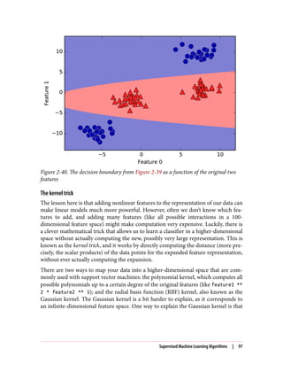
![11 This follows from the Taylor expansion of the exponential map.
it considers all possible polynomials of all degrees, but the importance of the features
decreases for higher degrees.11
In practice, the mathematical details behind the kernel SVM are not that important,
though, and how an SVM with an RBF kernel makes a decision can be summarized
quite easily—we’ll do so in the next section.
Understanding SVMs
During training, the SVM learns how important each of the training data points is to
represent the decision boundary between the two classes. Typically only a subset of
the training points matter for defining the decision boundary: the ones that lie on the
border between the classes. These are called support vectors and give the support vec‐
tor machine its name.
To make a prediction for a new point, the distance to each of the support vectors is
measured. A classification decision is made based on the distances to the support vec‐
tor, and the importance of the support vectors that was learned during training
(stored in the dual_coef_ attribute of SVC).
The distance between data points is measured by the Gaussian kernel:
krbf(x1, x2) = exp (ɣǁx1 - x2ǁ2
)
Here, x1 and x2 are data points, ǁ x1 - x2 ǁ denotes Euclidean distance, and ɣ (gamma)
is a parameter that controls the width of the Gaussian kernel.
Figure 2-41 shows the result of training a support vector machine on a two-
dimensional two-class dataset. The decision boundary is shown in black, and the sup‐
port vectors are larger points with the wide outline. The following code creates this
plot by training an SVM on the forge dataset:
In[81]:
from sklearn.svm import SVC
X, y = mglearn.tools.make_handcrafted_dataset()
svm = SVC(kernel='rbf', C=10, gamma=0.1).fit(X, y)
mglearn.plots.plot_2d_separator(svm, X, eps=.5)
mglearn.discrete_scatter(X[:, 0], X[:, 1], y)
# plot support vectors
sv = svm.support_vectors_
# class labels of support vectors are given by the sign of the dual coefficients
sv_labels = svm.dual_coef_.ravel() > 0
mglearn.discrete_scatter(sv[:, 0], sv[:, 1], sv_labels, s=15, markeredgewidth=3)
plt.xlabel("Feature 0")
plt.ylabel("Feature 1")
98 | Chapter 2: Supervised Learning](https://image.slidesharecdn.com/introductiontomachinelearningwithpythonpdfdrive-230107170822-bfb01dbd/85/Introduction-to-Machine-Learning-with-Python-PDFDrive-com-pdf-112-320.jpg)
![Figure 2-41. Decision boundary and support vectors found by an SVM with RBF kernel
In this case, the SVM yields a very smooth and nonlinear (not a straight line) bound‐
ary. We adjusted two parameters here: the C parameter and the gamma parameter,
which we will now discuss in detail.
Tuning SVM parameters
The gamma parameter is the one shown in the formula given in the previous section,
which controls the width of the Gaussian kernel. It determines the scale of what it
means for points to be close together. The C parameter is a regularization parameter,
similar to that used in the linear models. It limits the importance of each point (or
more precisely, their dual_coef_).
Let’s have a look at what happens when we vary these parameters (Figure 2-42):
In[82]:
fig, axes = plt.subplots(3, 3, figsize=(15, 10))
for ax, C in zip(axes, [-1, 0, 3]):
for a, gamma in zip(ax, range(-1, 2)):
mglearn.plots.plot_svm(log_C=C, log_gamma=gamma, ax=a)
axes[0, 0].legend(["class 0", "class 1", "sv class 0", "sv class 1"],
ncol=4, loc=(.9, 1.2))
Supervised Machine Learning Algorithms | 99](https://image.slidesharecdn.com/introductiontomachinelearningwithpythonpdfdrive-230107170822-bfb01dbd/85/Introduction-to-Machine-Learning-with-Python-PDFDrive-com-pdf-113-320.jpg)
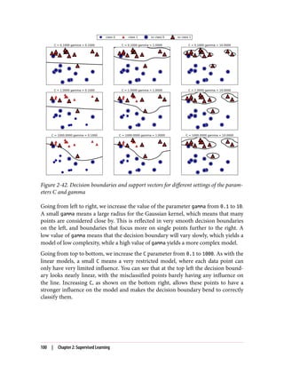
![Let’s apply the RBF kernel SVM to the Breast Cancer dataset. By default, C=1 and
gamma=1/n_features:
In[83]:
X_train, X_test, y_train, y_test = train_test_split(
cancer.data, cancer.target, random_state=0)
svc = SVC()
svc.fit(X_train, y_train)
print("Accuracy on training set: {:.2f}".format(svc.score(X_train, y_train)))
print("Accuracy on test set: {:.2f}".format(svc.score(X_test, y_test)))
Out[83]:
Accuracy on training set: 1.00
Accuracy on test set: 0.63
The model overfits quite substantially, with a perfect score on the training set and
only 63% accuracy on the test set. While SVMs often perform quite well, they are
very sensitive to the settings of the parameters and to the scaling of the data. In par‐
ticular, they require all the features to vary on a similar scale. Let’s look at the mini‐
mum and maximum values for each feature, plotted in log-space (Figure 2-43):
In[84]:
plt.plot(X_train.min(axis=0), 'o', label="min")
plt.plot(X_train.max(axis=0), '^', label="max")
plt.legend(loc=4)
plt.xlabel("Feature index")
plt.ylabel("Feature magnitude")
plt.yscale("log")
From this plot we can determine that features in the Breast Cancer dataset are of
completely different orders of magnitude. This can be somewhat of a problem for
other models (like linear models), but it has devastating effects for the kernel SVM.
Let’s examine some ways to deal with this issue.
Supervised Machine Learning Algorithms | 101](https://image.slidesharecdn.com/introductiontomachinelearningwithpythonpdfdrive-230107170822-bfb01dbd/85/Introduction-to-Machine-Learning-with-Python-PDFDrive-com-pdf-115-320.jpg)
![Figure 2-43. Feature ranges for the Breast Cancer dataset (note that the y axis has a log‐
arithmic scale)
Preprocessing data for SVMs
One way to resolve this problem is by rescaling each feature so that they are all
approximately on the same scale. A common rescaling method for kernel SVMs is to
scale the data such that all features are between 0 and 1. We will see how to do this
using the MinMaxScaler preprocessing method in Chapter 3, where we’ll give more
details. For now, let’s do this “by hand”:
In[85]:
# compute the minimum value per feature on the training set
min_on_training = X_train.min(axis=0)
# compute the range of each feature (max - min) on the training set
range_on_training = (X_train - min_on_training).max(axis=0)
# subtract the min, and divide by range
# afterward, min=0 and max=1 for each feature
X_train_scaled = (X_train - min_on_training) / range_on_training
print("Minimum for each featuren{}".format(X_train_scaled.min(axis=0)))
print("Maximum for each featuren {}".format(X_train_scaled.max(axis=0)))
102 | Chapter 2: Supervised Learning](https://image.slidesharecdn.com/introductiontomachinelearningwithpythonpdfdrive-230107170822-bfb01dbd/85/Introduction-to-Machine-Learning-with-Python-PDFDrive-com-pdf-116-320.jpg)
![Out[85]:
Minimum for each feature
[ 0. 0. 0. 0. 0. 0. 0. 0. 0. 0. 0. 0. 0. 0. 0. 0. 0. 0.
0. 0. 0. 0. 0. 0. 0. 0. 0. 0. 0. 0.]
Maximum for each feature
[ 1. 1. 1. 1. 1. 1. 1. 1. 1. 1. 1. 1. 1. 1. 1. 1. 1. 1.
1. 1. 1. 1. 1. 1. 1. 1. 1. 1. 1. 1.]
In[86]:
# use THE SAME transformation on the test set,
# using min and range of the training set (see Chapter 3 for details)
X_test_scaled = (X_test - min_on_training) / range_on_training
In[87]:
svc = SVC()
svc.fit(X_train_scaled, y_train)
print("Accuracy on training set: {:.3f}".format(
svc.score(X_train_scaled, y_train)))
print("Accuracy on test set: {:.3f}".format(svc.score(X_test_scaled, y_test)))
Out[87]:
Accuracy on training set: 0.948
Accuracy on test set: 0.951
Scaling the data made a huge difference! Now we are actually in an underfitting
regime, where training and test set performance are quite similar but less close to
100% accuracy. From here, we can try increasing either C or gamma to fit a more com‐
plex model. For example:
In[88]:
svc = SVC(C=1000)
svc.fit(X_train_scaled, y_train)
print("Accuracy on training set: {:.3f}".format(
svc.score(X_train_scaled, y_train)))
print("Accuracy on test set: {:.3f}".format(svc.score(X_test_scaled, y_test)))
Out[88]:
Accuracy on training set: 0.988
Accuracy on test set: 0.972
Here, increasing C allows us to improve the model significantly, resulting in 97.2%
accuracy.
Supervised Machine Learning Algorithms | 103](https://image.slidesharecdn.com/introductiontomachinelearningwithpythonpdfdrive-230107170822-bfb01dbd/85/Introduction-to-Machine-Learning-with-Python-PDFDrive-com-pdf-117-320.jpg)
![Remember that the prediction by a linear regressor is given as:
ŷ = w[0] * x[0] + w[1] * x[1] + ... + w[p] * x[p] + b
In plain English, ŷ is a weighted sum of the input features x[0] to x[p], weighted by
the learned coefficients w[0] to w[p]. We could visualize this graphically as shown in
Figure 2-44:
In[89]:
display(mglearn.plots.plot_logistic_regression_graph())
Figure 2-44. Visualization of logistic regression, where input features and predictions are
shown as nodes, and the coefficients are connections between the nodes
Here, each node on the left represents an input feature, the connecting lines represent
the learned coefficients, and the node on the right represents the output, which is a
weighted sum of the inputs.
In an MLP this process of computing weighted sums is repeated multiple times, first
computing hidden units that represent an intermediate processing step, which are
again combined using weighted sums to yield the final result (Figure 2-45):
In[90]:
display(mglearn.plots.plot_single_hidden_layer_graph())
Supervised Machine Learning Algorithms | 105](https://image.slidesharecdn.com/introductiontomachinelearningwithpythonpdfdrive-230107170822-bfb01dbd/85/Introduction-to-Machine-Learning-with-Python-PDFDrive-com-pdf-119-320.jpg)
![Figure 2-45. Illustration of a multilayer perceptron with a single hidden layer
This model has a lot more coefficients (also called weights) to learn: there is one
between every input and every hidden unit (which make up the hidden layer), and
one between every unit in the hidden layer and the output.
Computing a series of weighted sums is mathematically the same as computing just
one weighted sum, so to make this model truly more powerful than a linear model,
we need one extra trick. After computing a weighted sum for each hidden unit, a
nonlinear function is applied to the result—usually the rectifying nonlinearity (also
known as rectified linear unit or relu) or the tangens hyperbolicus (tanh). The result of
this function is then used in the weighted sum that computes the output, ŷ. The two
functions are visualized in Figure 2-46. The relu cuts off values below zero, while tanh
saturates to –1 for low input values and +1 for high input values. Either nonlinear
function allows the neural network to learn much more complicated functions than a
linear model could:
In[91]:
line = np.linspace(-3, 3, 100)
plt.plot(line, np.tanh(line), label="tanh")
plt.plot(line, np.maximum(line, 0), label="relu")
plt.legend(loc="best")
plt.xlabel("x")
plt.ylabel("relu(x), tanh(x)")
106 | Chapter 2: Supervised Learning](https://image.slidesharecdn.com/introductiontomachinelearningwithpythonpdfdrive-230107170822-bfb01dbd/85/Introduction-to-Machine-Learning-with-Python-PDFDrive-com-pdf-120-320.jpg)
![Figure 2-46. The hyperbolic tangent activation function and the rectified linear activa‐
tion function
For the small neural network pictured in Figure 2-45, the full formula for computing
ŷ in the case of regression would be (when using a tanh nonlinearity):
h[0] = tanh(w[0, 0] * x[0] + w[1, 0] * x[1] + w[2, 0] * x[2] + w[3, 0] * x[3])
h[1] = tanh(w[0, 0] * x[0] + w[1, 0] * x[1] + w[2, 0] * x[2] + w[3, 0] * x[3])
h[2] = tanh(w[0, 0] * x[0] + w[1, 0] * x[1] + w[2, 0] * x[2] + w[3, 0] * x[3])
ŷ = v[0] * h[0] + v[1] * h[1] + v[2] * h[2]
Here, w are the weights between the input x and the hidden layer h, and v are the
weights between the hidden layer h and the output ŷ. The weights v and w are learned
from data, x are the input features, ŷ is the computed output, and h are intermediate
computations. An important parameter that needs to be set by the user is the number
of nodes in the hidden layer. This can be as small as 10 for very small or simple data‐
sets and as big as 10,000 for very complex data. It is also possible to add additional
hidden layers, as shown in Figure 2-47:
Supervised Machine Learning Algorithms | 107](https://image.slidesharecdn.com/introductiontomachinelearningwithpythonpdfdrive-230107170822-bfb01dbd/85/Introduction-to-Machine-Learning-with-Python-PDFDrive-com-pdf-121-320.jpg)
![In[92]:
mglearn.plots.plot_two_hidden_layer_graph()
Figure 2-47. A multilayer perceptron with two hidden layers
Having large neural networks made up of many of these layers of computation is
what inspired the term “deep learning.”
Tuning neural networks
Let’s look into the workings of the MLP by applying the MLPClassifier to the
two_moons dataset we used earlier in this chapter. The results are shown in
Figure 2-48:
In[93]:
from sklearn.neural_network import MLPClassifier
from sklearn.datasets import make_moons
X, y = make_moons(n_samples=100, noise=0.25, random_state=3)
X_train, X_test, y_train, y_test = train_test_split(X, y, stratify=y,
random_state=42)
mlp = MLPClassifier(algorithm='l-bfgs', random_state=0).fit(X_train, y_train)
mglearn.plots.plot_2d_separator(mlp, X_train, fill=True, alpha=.3)
mglearn.discrete_scatter(X_train[:, 0], X_train[:, 1], y_train)
plt.xlabel("Feature 0")
plt.ylabel("Feature 1")
108 | Chapter 2: Supervised Learning](https://image.slidesharecdn.com/introductiontomachinelearningwithpythonpdfdrive-230107170822-bfb01dbd/85/Introduction-to-Machine-Learning-with-Python-PDFDrive-com-pdf-122-320.jpg)
![Figure 2-48. Decision boundary learned by a neural network with 100 hidden units on
the two_moons dataset
As you can see, the neural network learned a very nonlinear but relatively smooth
decision boundary. We used algorithm='l-bfgs', which we will discuss later.
By default, the MLP uses 100 hidden nodes, which is quite a lot for this small dataset.
We can reduce the number (which reduces the complexity of the model) and still get
a good result (Figure 2-49):
In[94]:
mlp = MLPClassifier(algorithm='l-bfgs', random_state=0, hidden_layer_sizes=[10])
mlp.fit(X_train, y_train)
mglearn.plots.plot_2d_separator(mlp, X_train, fill=True, alpha=.3)
mglearn.discrete_scatter(X_train[:, 0], X_train[:, 1], y_train)
plt.xlabel("Feature 0")
plt.ylabel("Feature 1")
Supervised Machine Learning Algorithms | 109](https://image.slidesharecdn.com/introductiontomachinelearningwithpythonpdfdrive-230107170822-bfb01dbd/85/Introduction-to-Machine-Learning-with-Python-PDFDrive-com-pdf-123-320.jpg)
![Figure 2-49. Decision boundary learned by a neural network with 10 hidden units on
the two_moons dataset
With only 10 hidden units, the decision boundary looks somewhat more ragged. The
default nonlinearity is relu, shown in Figure 2-46. With a single hidden layer, this
means the decision function will be made up of 10 straight line segments. If we want
a smoother decision boundary, we could add more hidden units (as in Figure 2-49),
add a second hidden layer (Figure 2-50), or use the tanh nonlinearity (Figure 2-51):
In[95]:
# using two hidden layers, with 10 units each
mlp = MLPClassifier(algorithm='l-bfgs', random_state=0,
hidden_layer_sizes=[10, 10])
mlp.fit(X_train, y_train)
mglearn.plots.plot_2d_separator(mlp, X_train, fill=True, alpha=.3)
mglearn.discrete_scatter(X_train[:, 0], X_train[:, 1], y_train)
plt.xlabel("Feature 0")
plt.ylabel("Feature 1")
110 | Chapter 2: Supervised Learning](https://image.slidesharecdn.com/introductiontomachinelearningwithpythonpdfdrive-230107170822-bfb01dbd/85/Introduction-to-Machine-Learning-with-Python-PDFDrive-com-pdf-124-320.jpg)
![In[96]:
# using two hidden layers, with 10 units each, now with tanh nonlinearity
mlp = MLPClassifier(algorithm='l-bfgs', activation='tanh',
random_state=0, hidden_layer_sizes=[10, 10])
mlp.fit(X_train, y_train)
mglearn.plots.plot_2d_separator(mlp, X_train, fill=True, alpha=.3)
mglearn.discrete_scatter(X_train[:, 0], X_train[:, 1], y_train)
plt.xlabel("Feature 0")
plt.ylabel("Feature 1")
Figure 2-50. Decision boundary learned using 2 hidden layers with 10 hidden units
each, with rect activation function
Supervised Machine Learning Algorithms | 111](https://image.slidesharecdn.com/introductiontomachinelearningwithpythonpdfdrive-230107170822-bfb01dbd/85/Introduction-to-Machine-Learning-with-Python-PDFDrive-com-pdf-125-320.jpg)
![Figure 2-51. Decision boundary learned using 2 hidden layers with 10 hidden units
each, with tanh activation function
Finally, we can also control the complexity of a neural network by using an l2 penalty
to shrink the weights toward zero, as we did in ridge regression and the linear classifi‐
ers. The parameter for this in the MLPClassifier is alpha (as in the linear regression
models), and it’s set to a very low value (little regularization) by default. Figure 2-52
shows the effect of different values of alpha on the two_moons dataset, using two hid‐
den layers of 10 or 100 units each:
In[97]:
fig, axes = plt.subplots(2, 4, figsize=(20, 8))
for axx, n_hidden_nodes in zip(axes, [10, 100]):
for ax, alpha in zip(axx, [0.0001, 0.01, 0.1, 1]):
mlp = MLPClassifier(algorithm='l-bfgs', random_state=0,
hidden_layer_sizes=[n_hidden_nodes, n_hidden_nodes],
alpha=alpha)
mlp.fit(X_train, y_train)
mglearn.plots.plot_2d_separator(mlp, X_train, fill=True, alpha=.3, ax=ax)
mglearn.discrete_scatter(X_train[:, 0], X_train[:, 1], y_train, ax=ax)
ax.set_title("n_hidden=[{}, {}]nalpha={:.4f}".format(
n_hidden_nodes, n_hidden_nodes, alpha))
112 | Chapter 2: Supervised Learning](https://image.slidesharecdn.com/introductiontomachinelearningwithpythonpdfdrive-230107170822-bfb01dbd/85/Introduction-to-Machine-Learning-with-Python-PDFDrive-com-pdf-126-320.jpg)
![Figure 2-52. Decision functions for different numbers of hidden units and different set‐
tings of the alpha parameter
As you probably have realized by now, there are many ways to control the complexity
of a neural network: the number of hidden layers, the number of units in each hidden
layer, and the regularization (alpha). There are actually even more, which we won’t
go into here.
An important property of neural networks is that their weights are set randomly
before learning is started, and this random initialization affects the model that is
learned. That means that even when using exactly the same parameters, we can
obtain very different models when using different random seeds. If the networks are
large, and their complexity is chosen properly, this should not affect accuracy too
much, but it is worth keeping in mind (particularly for smaller networks).
Figure 2-53 shows plots of several models, all learned with the same settings of the
parameters:
In[98]:
fig, axes = plt.subplots(2, 4, figsize=(20, 8))
for i, ax in enumerate(axes.ravel()):
mlp = MLPClassifier(algorithm='l-bfgs', random_state=i,
hidden_layer_sizes=[100, 100])
mlp.fit(X_train, y_train)
mglearn.plots.plot_2d_separator(mlp, X_train, fill=True, alpha=.3, ax=ax)
mglearn.discrete_scatter(X_train[:, 0], X_train[:, 1], y_train, ax=ax)
Supervised Machine Learning Algorithms | 113](https://image.slidesharecdn.com/introductiontomachinelearningwithpythonpdfdrive-230107170822-bfb01dbd/85/Introduction-to-Machine-Learning-with-Python-PDFDrive-com-pdf-127-320.jpg)
![Figure 2-53. Decision functions learned with the same parameters but different random
initializations
To get a better understanding of neural networks on real-world data, let’s apply the
MLPClassifier to the Breast Cancer dataset. We start with the default parameters:
In[99]:
print("Cancer data per-feature maxima:n{}".format(cancer.data.max(axis=0)))
Out[99]:
Cancer data per-feature maxima:
[ 28.110 39.280 188.500 2501.000 0.163 0.345 0.427
0.201 0.304 0.097 2.873 4.885 21.980 542.200
0.031 0.135 0.396 0.053 0.079 0.030 36.040
49.540 251.200 4254.000 0.223 1.058 1.252 0.291
0.664 0.207]
In[100]:
X_train, X_test, y_train, y_test = train_test_split(
cancer.data, cancer.target, random_state=0)
mlp = MLPClassifier(random_state=42)
mlp.fit(X_train, y_train)
print("Accuracy on training set: {:.2f}".format(mlp.score(X_train, y_train)))
print("Accuracy on test set: {:.2f}".format(mlp.score(X_test, y_test)))
Out[100]:
Accuracy on training set: 0.92
Accuracy on test set: 0.90
The accuracy of the MLP is quite good, but not as good as the other models. As in the
earlier SVC example, this is likely due to scaling of the data. Neural networks also
expect all input features to vary in a similar way, and ideally to have a mean of 0, and
114 | Chapter 2: Supervised Learning](https://image.slidesharecdn.com/introductiontomachinelearningwithpythonpdfdrive-230107170822-bfb01dbd/85/Introduction-to-Machine-Learning-with-Python-PDFDrive-com-pdf-128-320.jpg)
![a variance of 1. We must rescale our data so that it fulfills these requirements. Again,
we will do this by hand here, but we’ll introduce the StandardScaler to do this auto‐
matically in Chapter 3:
In[101]:
# compute the mean value per feature on the training set
mean_on_train = X_train.mean(axis=0)
# compute the standard deviation of each feature on the training set
std_on_train = X_train.std(axis=0)
# subtract the mean, and scale by inverse standard deviation
# afterward, mean=0 and std=1
X_train_scaled = (X_train - mean_on_train) / std_on_train
# use THE SAME transformation (using training mean and std) on the test set
X_test_scaled = (X_test - mean_on_train) / std_on_train
mlp = MLPClassifier(random_state=0)
mlp.fit(X_train_scaled, y_train)
print("Accuracy on training set: {:.3f}".format(
mlp.score(X_train_scaled, y_train)))
print("Accuracy on test set: {:.3f}".format(mlp.score(X_test_scaled, y_test)))
Out[101]:
Accuracy on training set: 0.991
Accuracy on test set: 0.965
ConvergenceWarning:
Stochastic Optimizer: Maximum iterations reached and the optimization
hasn't converged yet.
The results are much better after scaling, and already quite competitive. We got a
warning from the model, though, that tells us that the maximum number of iterations
has been reached. This is part of the adam algorithm for learning the model, and tells
us that we should increase the number of iterations:
In[102]:
mlp = MLPClassifier(max_iter=1000, random_state=0)
mlp.fit(X_train_scaled, y_train)
print("Accuracy on training set: {:.3f}".format(
mlp.score(X_train_scaled, y_train)))
print("Accuracy on test set: {:.3f}".format(mlp.score(X_test_scaled, y_test)))
Out[102]:
Accuracy on training set: 0.995
Accuracy on test set: 0.965
Supervised Machine Learning Algorithms | 115](https://image.slidesharecdn.com/introductiontomachinelearningwithpythonpdfdrive-230107170822-bfb01dbd/85/Introduction-to-Machine-Learning-with-Python-PDFDrive-com-pdf-129-320.jpg)
![12 You might have noticed at this point that many of the well-performing models achieved exactly the same
accuracy of 0.972. This means that all of the models make exactly the same number of mistakes, which is four.
If you compare the actual predictions, you can even see that they make exactly the same mistakes! This might
be a consequence of the dataset being very small, or it may be because these points are really different from
the rest.
Increasing the number of iterations only increased the training set performance, not
the generalization performance. Still, the model is performing quite well. As there is
some gap between the training and the test performance, we might try to decrease the
model’s complexity to get better generalization performance. Here, we choose to
increase the alpha parameter (quite aggressively, from 0.0001 to 1) to add stronger
regularization of the weights:
In[103]:
mlp = MLPClassifier(max_iter=1000, alpha=1, random_state=0)
mlp.fit(X_train_scaled, y_train)
print("Accuracy on training set: {:.3f}".format(
mlp.score(X_train_scaled, y_train)))
print("Accuracy on test set: {:.3f}".format(mlp.score(X_test_scaled, y_test)))
Out[103]:
Accuracy on training set: 0.988
Accuracy on test set: 0.972
This leads to a performance on par with the best models so far.12
While it is possible to analyze what a neural network has learned, this is usually much
trickier than analyzing a linear model or a tree-based model. One way to introspect
what was learned is to look at the weights in the model. You can see an example of
this in the scikit-learn example gallery. For the Breast Cancer dataset, this might
be a bit hard to understand. The following plot (Figure 2-54) shows the weights that
were learned connecting the input to the first hidden layer. The rows in this plot cor‐
respond to the 30 input features, while the columns correspond to the 100 hidden
units. Light colors represent large positive values, while dark colors represent nega‐
tive values:
In[104]:
plt.figure(figsize=(20, 5))
plt.imshow(mlp.coefs_[0], interpolation='none', cmap='viridis')
plt.yticks(range(30), cancer.feature_names)
plt.xlabel("Columns in weight matrix")
plt.ylabel("Input feature")
plt.colorbar()
116 | Chapter 2: Supervised Learning](https://image.slidesharecdn.com/introductiontomachinelearningwithpythonpdfdrive-230107170822-bfb01dbd/85/Introduction-to-Machine-Learning-with-Python-PDFDrive-com-pdf-130-320.jpg)
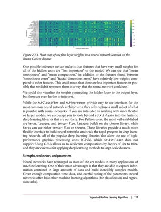
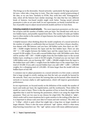
![eters that need to be tuned for best results. You can find all of these parameters and
their definitions in the user guide. When starting to work with MLPs, we recommend
sticking to 'adam' and 'l-bfgs'.
fit Resets a Model
An important property of scikit-learn models is that calling fit
will always reset everything a model previously learned. So if you
build a model on one dataset, and then call fit again on a different
dataset, the model will “forget” everything it learned from the first
dataset. You can call fit as often as you like on a model, and the
outcome will be the same as calling fit on a “new” model.
Uncertainty Estimates from Classifiers
Another useful part of the scikit-learn interface that we haven’t talked about yet is
the ability of classifiers to provide uncertainty estimates of predictions. Often, you are
not only interested in which class a classifier predicts for a certain test point, but also
how certain it is that this is the right class. In practice, different kinds of mistakes lead
to very different outcomes in real-world applications. Imagine a medical application
testing for cancer. Making a false positive prediction might lead to a patient undergo‐
ing additional tests, while a false negative prediction might lead to a serious disease
not being treated. We will go into this topic in more detail in Chapter 6.
There are two different functions in scikit-learn that can be used to obtain uncer‐
tainty estimates from classifiers: decision_function and predict_proba. Most (but
not all) classifiers have at least one of them, and many classifiers have both. Let’s look
at what these two functions do on a synthetic two-dimensional dataset, when build‐
ing a GradientBoostingClassifier classifier, which has both a decision_function
and a predict_proba method:
In[105]:
from sklearn.ensemble import GradientBoostingClassifier
from sklearn.datasets import make_blobs, make_circles
X, y = make_circles(noise=0.25, factor=0.5, random_state=1)
# we rename the classes "blue" and "red" for illustration purposes
y_named = np.array(["blue", "red"])[y]
# we can call train_test_split with arbitrarily many arrays;
# all will be split in a consistent manner
X_train, X_test, y_train_named, y_test_named, y_train, y_test =
train_test_split(X, y_named, y, random_state=0)
# build the gradient boosting model
gbrt = GradientBoostingClassifier(random_state=0)
gbrt.fit(X_train, y_train_named)
Uncertainty Estimates from Classifiers | 119](https://image.slidesharecdn.com/introductiontomachinelearningwithpythonpdfdrive-230107170822-bfb01dbd/85/Introduction-to-Machine-Learning-with-Python-PDFDrive-com-pdf-133-320.jpg)
![The Decision Function
In the binary classification case, the return value of decision_function is of shape
(n_samples,), and it returns one floating-point number for each sample:
In[106]:
print("X_test.shape: {}".format(X_test.shape))
print("Decision function shape: {}".format(
gbrt.decision_function(X_test).shape))
Out[106]:
X_test.shape: (25, 2)
Decision function shape: (25,)
This value encodes how strongly the model believes a data point to belong to the
“positive” class, in this case class 1. Positive values indicate a preference for the posi‐
tive class, and negative values indicate a preference for the “negative” (other) class:
In[107]:
# show the first few entries of decision_function
print("Decision function:n{}".format(gbrt.decision_function(X_test)[:6]))
Out[107]:
Decision function:
[ 4.136 -1.683 -3.951 -3.626 4.29 3.662]
We can recover the prediction by looking only at the sign of the decision function:
In[108]:
print("Thresholded decision function:n{}".format(
gbrt.decision_function(X_test) > 0))
print("Predictions:n{}".format(gbrt.predict(X_test)))
Out[108]:
Thresholded decision function:
[ True False False False True True False True True True False True
True False True False False False True True True True True False
False]
Predictions:
['red' 'blue' 'blue' 'blue' 'red' 'red' 'blue' 'red' 'red' 'red' 'blue'
'red' 'red' 'blue' 'red' 'blue' 'blue' 'blue' 'red' 'red' 'red' 'red'
'red' 'blue' 'blue']
For binary classification, the “negative” class is always the first entry of the classes_
attribute, and the “positive” class is the second entry of classes_. So if you want to
fully recover the output of predict, you need to make use of the classes_ attribute:
120 | Chapter 2: Supervised Learning](https://image.slidesharecdn.com/introductiontomachinelearningwithpythonpdfdrive-230107170822-bfb01dbd/85/Introduction-to-Machine-Learning-with-Python-PDFDrive-com-pdf-134-320.jpg)
![In[109]:
# make the boolean True/False into 0 and 1
greater_zero = (gbrt.decision_function(X_test) > 0).astype(int)
# use 0 and 1 as indices into classes_
pred = gbrt.classes_[greater_zero]
# pred is the same as the output of gbrt.predict
print("pred is equal to predictions: {}".format(
np.all(pred == gbrt.predict(X_test))))
Out[109]:
pred is equal to predictions: True
The range of decision_function can be arbitrary, and depends on the data and the
model parameters:
In[110]:
decision_function = gbrt.decision_function(X_test)
print("Decision function minimum: {:.2f} maximum: {:.2f}".format(
np.min(decision_function), np.max(decision_function)))
Out[110]:
Decision function minimum: -7.69 maximum: 4.29
This arbitrary scaling makes the output of decision_function often hard to
interpret.
In the following example we plot the decision_function for all points in the 2D
plane using a color coding, next to a visualization of the decision boundary, as we saw
earlier. We show training points as circles and test data as triangles (Figure 2-55):
In[111]:
fig, axes = plt.subplots(1, 2, figsize=(13, 5))
mglearn.tools.plot_2d_separator(gbrt, X, ax=axes[0], alpha=.4,
fill=True, cm=mglearn.cm2)
scores_image = mglearn.tools.plot_2d_scores(gbrt, X, ax=axes[1],
alpha=.4, cm=mglearn.ReBl)
for ax in axes:
# plot training and test points
mglearn.discrete_scatter(X_test[:, 0], X_test[:, 1], y_test,
markers='^', ax=ax)
mglearn.discrete_scatter(X_train[:, 0], X_train[:, 1], y_train,
markers='o', ax=ax)
ax.set_xlabel("Feature 0")
ax.set_ylabel("Feature 1")
cbar = plt.colorbar(scores_image, ax=axes.tolist())
axes[0].legend(["Test class 0", "Test class 1", "Train class 0",
"Train class 1"], ncol=4, loc=(.1, 1.1))
Uncertainty Estimates from Classifiers | 121](https://image.slidesharecdn.com/introductiontomachinelearningwithpythonpdfdrive-230107170822-bfb01dbd/85/Introduction-to-Machine-Learning-with-Python-PDFDrive-com-pdf-135-320.jpg)
![Figure 2-55. Decision boundary (left) and decision function (right) for a gradient boost‐
ing model on a two-dimensional toy dataset
Encoding not only the predicted outcome but also how certain the classifier is pro‐
vides additional information. However, in this visualization, it is hard to make out the
boundary between the two classes.
Predicting Probabilities
The output of predict_proba is a probability for each class, and is often more easily
understood than the output of decision_function. It is always of shape (n_samples,
2) for binary classification:
In[112]:
print("Shape of probabilities: {}".format(gbrt.predict_proba(X_test).shape))
Out[112]:
Shape of probabilities: (25, 2)
The first entry in each row is the estimated probability of the first class, and the sec‐
ond entry is the estimated probability of the second class. Because it is a probability,
the output of predict_proba is always between 0 and 1, and the sum of the entries
for both classes is always 1:
In[113]:
# show the first few entries of predict_proba
print("Predicted probabilities:n{}".format(
gbrt.predict_proba(X_test[:6])))
122 | Chapter 2: Supervised Learning](https://image.slidesharecdn.com/introductiontomachinelearningwithpythonpdfdrive-230107170822-bfb01dbd/85/Introduction-to-Machine-Learning-with-Python-PDFDrive-com-pdf-136-320.jpg)
![13 Because the probabilities are floating-point numbers, it is unlikely that they will both be exactly 0.500. How‐
ever, if that happens, the prediction is made at random.
Out[113]:
Predicted probabilities:
[[ 0.016 0.984]
[ 0.843 0.157]
[ 0.981 0.019]
[ 0.974 0.026]
[ 0.014 0.986]
[ 0.025 0.975]]
Because the probabilities for the two classes sum to 1, exactly one of the classes will
be above 50% certainty. That class is the one that is predicted.13
You can see in the previous output that the classifier is relatively certain for most
points. How well the uncertainty actually reflects uncertainty in the data depends on
the model and the parameters. A model that is more overfitted tends to make more
certain predictions, even if they might be wrong. A model with less complexity usu‐
ally has more uncertainty in its predictions. A model is called calibrated if the
reported uncertainty actually matches how correct it is—in a calibrated model, a pre‐
diction made with 70% certainty would be correct 70% of the time.
In the following example (Figure 2-56) we again show the decision boundary on the
dataset, next to the class probabilities for the class 1:
In[114]:
fig, axes = plt.subplots(1, 2, figsize=(13, 5))
mglearn.tools.plot_2d_separator(
gbrt, X, ax=axes[0], alpha=.4, fill=True, cm=mglearn.cm2)
scores_image = mglearn.tools.plot_2d_scores(
gbrt, X, ax=axes[1], alpha=.5, cm=mglearn.ReBl, function='predict_proba')
for ax in axes:
# plot training and test points
mglearn.discrete_scatter(X_test[:, 0], X_test[:, 1], y_test,
markers='^', ax=ax)
mglearn.discrete_scatter(X_train[:, 0], X_train[:, 1], y_train,
markers='o', ax=ax)
ax.set_xlabel("Feature 0")
ax.set_ylabel("Feature 1")
cbar = plt.colorbar(scores_image, ax=axes.tolist())
axes[0].legend(["Test class 0", "Test class 1", "Train class 0",
"Train class 1"], ncol=4, loc=(.1, 1.1))
Uncertainty Estimates from Classifiers | 123](https://image.slidesharecdn.com/introductiontomachinelearningwithpythonpdfdrive-230107170822-bfb01dbd/85/Introduction-to-Machine-Learning-with-Python-PDFDrive-com-pdf-137-320.jpg)
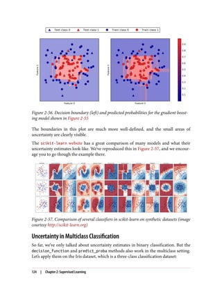
![In[115]:
from sklearn.datasets import load_iris
iris = load_iris()
X_train, X_test, y_train, y_test = train_test_split(
iris.data, iris.target, random_state=42)
gbrt = GradientBoostingClassifier(learning_rate=0.01, random_state=0)
gbrt.fit(X_train, y_train)
In[116]:
print("Decision function shape: {}".format(gbrt.decision_function(X_test).shape))
# plot the first few entries of the decision function
print("Decision function:n{}".format(gbrt.decision_function(X_test)[:6, :]))
Out[116]:
Decision function shape: (38, 3)
Decision function:
[[-0.529 1.466 -0.504]
[ 1.512 -0.496 -0.503]
[-0.524 -0.468 1.52 ]
[-0.529 1.466 -0.504]
[-0.531 1.282 0.215]
[ 1.512 -0.496 -0.503]]
In the multiclass case, the decision_function has the shape (n_samples,
n_classes) and each column provides a “certainty score” for each class, where a large
score means that a class is more likely and a small score means the class is less likely.
You can recover the predictions from these scores by finding the maximum entry for
each data point:
In[117]:
print("Argmax of decision function:n{}".format(
np.argmax(gbrt.decision_function(X_test), axis=1)))
print("Predictions:n{}".format(gbrt.predict(X_test)))
Out[117]:
Argmax of decision function:
[1 0 2 1 1 0 1 2 1 1 2 0 0 0 0 1 2 1 1 2 0 2 0 2 2 2 2 2 0 0 0 0 1 0 0 2 1 0]
Predictions:
[1 0 2 1 1 0 1 2 1 1 2 0 0 0 0 1 2 1 1 2 0 2 0 2 2 2 2 2 0 0 0 0 1 0 0 2 1 0]
The output of predict_proba has the same shape, (n_samples, n_classes). Again,
the probabilities for the possible classes for each data point sum to 1:
Uncertainty Estimates from Classifiers | 125](https://image.slidesharecdn.com/introductiontomachinelearningwithpythonpdfdrive-230107170822-bfb01dbd/85/Introduction-to-Machine-Learning-with-Python-PDFDrive-com-pdf-139-320.jpg)
![In[118]:
# show the first few entries of predict_proba
print("Predicted probabilities:n{}".format(gbrt.predict_proba(X_test)[:6]))
# show that sums across rows are one
print("Sums: {}".format(gbrt.predict_proba(X_test)[:6].sum(axis=1)))
Out[118]:
Predicted probabilities:
[[ 0.107 0.784 0.109]
[ 0.789 0.106 0.105]
[ 0.102 0.108 0.789]
[ 0.107 0.784 0.109]
[ 0.108 0.663 0.228]
[ 0.789 0.106 0.105]]
Sums: [ 1. 1. 1. 1. 1. 1.]
We can again recover the predictions by computing the argmax of predict_proba:
In[119]:
print("Argmax of predicted probabilities:n{}".format(
np.argmax(gbrt.predict_proba(X_test), axis=1)))
print("Predictions:n{}".format(gbrt.predict(X_test)))
Out[119]:
Argmax of predicted probabilities:
[1 0 2 1 1 0 1 2 1 1 2 0 0 0 0 1 2 1 1 2 0 2 0 2 2 2 2 2 0 0 0 0 1 0 0 2 1 0]
Predictions:
[1 0 2 1 1 0 1 2 1 1 2 0 0 0 0 1 2 1 1 2 0 2 0 2 2 2 2 2 0 0 0 0 1 0 0 2 1 0]
To summarize, predict_proba and decision_function always have shape (n_sam
ples, n_classes)—apart from decision_function in the special binary case. In the
binary case, decision_function only has one column, corresponding to the “posi‐
tive” class classes_[1]. This is mostly for historical reasons.
You can recover the prediction when there are n_classes many columns by comput‐
ing the argmax across columns. Be careful, though, if your classes are strings, or you
use integers but they are not consecutive and starting from 0. If you want to compare
results obtained with predict to results obtained via decision_function or pre
dict_proba, make sure to use the classes_ attribute of the classifier to get the actual
class names:
126 | Chapter 2: Supervised Learning](https://image.slidesharecdn.com/introductiontomachinelearningwithpythonpdfdrive-230107170822-bfb01dbd/85/Introduction-to-Machine-Learning-with-Python-PDFDrive-com-pdf-140-320.jpg)
![In[120]:
logreg = LogisticRegression()
# represent each target by its class name in the iris dataset
named_target = iris.target_names[y_train]
logreg.fit(X_train, named_target)
print("unique classes in training data: {}".format(logreg.classes_))
print("predictions: {}".format(logreg.predict(X_test)[:10]))
argmax_dec_func = np.argmax(logreg.decision_function(X_test), axis=1)
print("argmax of decision function: {}".format(argmax_dec_func[:10]))
print("argmax combined with classes_: {}".format(
logreg.classes_[argmax_dec_func][:10]))
Out[120]:
unique classes in training data: ['setosa' 'versicolor' 'virginica']
predictions: ['versicolor' 'setosa' 'virginica' 'versicolor' 'versicolor'
'setosa' 'versicolor' 'virginica' 'versicolor' 'versicolor']
argmax of decision function: [1 0 2 1 1 0 1 2 1 1]
argmax combined with classes_: ['versicolor' 'setosa' 'virginica' 'versicolor'
'versicolor' 'setosa' 'versicolor' 'virginica' 'versicolor' 'versicolor']
Summary and Outlook
We started this chapter with a discussion of model complexity, then discussed gener‐
alization, or learning a model that is able to perform well on new, previously unseen
data. This led us to the concepts of underfitting, which describes a model that cannot
capture the variations present in the training data, and overfitting, which describes a
model that focuses too much on the training data and is not able to generalize to new
data very well.
We then discussed a wide array of machine learning models for classification and
regression, what their advantages and disadvantages are, and how to control model
complexity for each of them. We saw that for many of the algorithms, setting the right
parameters is important for good performance. Some of the algorithms are also sensi‐
tive to how we represent the input data, and in particular to how the features are
scaled. Therefore, blindly applying an algorithm to a dataset without understanding
the assumptions the model makes and the meanings of the parameter settings will
rarely lead to an accurate model.
This chapter contains a lot of information about the algorithms, and it is not neces‐
sary for you to remember all of these details for the following chapters. However,
some knowledge of the models described here—and which to use in a specific situa‐
tion—is important for successfully applying machine learning in practice. Here is a
quick summary of when to use each model:
Summary and Outlook | 127](https://image.slidesharecdn.com/introductiontomachinelearningwithpythonpdfdrive-230107170822-bfb01dbd/85/Introduction-to-Machine-Learning-with-Python-PDFDrive-com-pdf-141-320.jpg)
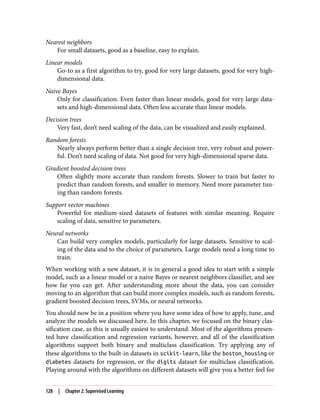


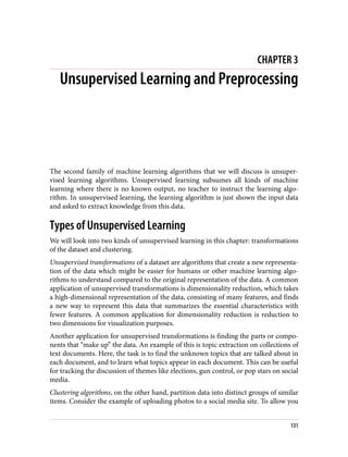
![to organize your pictures, the site might want to group together pictures that show
the same person. However, the site doesn’t know which pictures show whom, and it
doesn’t know how many different people appear in your photo collection. A sensible
approach would be to extract all the faces and divide them into groups of faces that
look similar. Hopefully, these correspond to the same person, and the images can be
grouped together for you.
Challenges in Unsupervised Learning
A major challenge in unsupervised learning is evaluating whether the algorithm
learned something useful. Unsupervised learning algorithms are usually applied to
data that does not contain any label information, so we don’t know what the right
output should be. Therefore, it is very hard to say whether a model “did well.” For
example, our hypothetical clustering algorithm could have grouped together all the
pictures that show faces in profile and all the full-face pictures. This would certainly
be a possible way to divide a collection of pictures of people’s faces, but it’s not the one
we were looking for. However, there is no way for us to “tell” the algorithm what we
are looking for, and often the only way to evaluate the result of an unsupervised algo‐
rithm is to inspect it manually.
As a consequence, unsupervised algorithms are used often in an exploratory setting,
when a data scientist wants to understand the data better, rather than as part of a
larger automatic system. Another common application for unsupervised algorithms
is as a preprocessing step for supervised algorithms. Learning a new representation of
the data can sometimes improve the accuracy of supervised algorithms, or can lead to
reduced memory and time consumption.
Before we start with “real” unsupervised algorithms, we will briefly discuss some sim‐
ple preprocessing methods that often come in handy. Even though preprocessing and
scaling are often used in tandem with supervised learning algorithms, scaling meth‐
ods don’t make use of the supervised information, making them unsupervised.
Preprocessing and Scaling
In the previous chapter we saw that some algorithms, like neural networks and SVMs,
are very sensitive to the scaling of the data. Therefore, a common practice is to adjust
the features so that the data representation is more suitable for these algorithms.
Often, this is a simple per-feature rescaling and shift of the data. The following code
(Figure 3-1) shows a simple example:
In[2]:
mglearn.plots.plot_scaling()
132 | Chapter 3: Unsupervised Learning and Preprocessing](https://image.slidesharecdn.com/introductiontomachinelearningwithpythonpdfdrive-230107170822-bfb01dbd/85/Introduction-to-Machine-Learning-with-Python-PDFDrive-com-pdf-146-320.jpg)
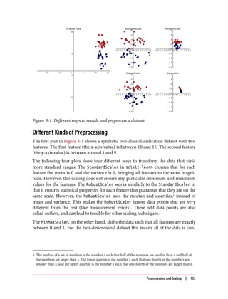
![tained within the rectangle created by the x-axis between 0 and 1 and the y-axis
between 0 and 1.
Finally, the Normalizer does a very different kind of rescaling. It scales each data
point such that the feature vector has a Euclidean length of 1. In other words, it
projects a data point on the circle (or sphere, in the case of higher dimensions) with a
radius of 1. This means every data point is scaled by a different number (by the
inverse of its length). This normalization is often used when only the direction (or
angle) of the data matters, not the length of the feature vector.
Applying Data Transformations
Now that we’ve seen what the different kinds of transformations do, let’s apply them
using scikit-learn. We will use the cancer dataset that we saw in Chapter 2. Pre‐
processing methods like the scalers are usually applied before applying a supervised
machine learning algorithm. As an example, say we want to apply the kernel SVM
(SVC) to the cancer dataset, and use MinMaxScaler for preprocessing the data. We
start by loading our dataset and splitting it into a training set and a test set (we need
separate training and test sets to evaluate the supervised model we will build after the
preprocessing):
In[3]:
from sklearn.datasets import load_breast_cancer
from sklearn.model_selection import train_test_split
cancer = load_breast_cancer()
X_train, X_test, y_train, y_test = train_test_split(cancer.data, cancer.target,
random_state=1)
print(X_train.shape)
print(X_test.shape)
Out[3]:
(426, 30)
(143, 30)
As a reminder, the dataset contains 569 data points, each represented by 30 measure‐
ments. We split the dataset into 426 samples for the training set and 143 samples for
the test set.
As with the supervised models we built earlier, we first import the class that imple‐
ments the preprocessing, and then instantiate it:
In[4]:
from sklearn.preprocessing import MinMaxScaler
scaler = MinMaxScaler()
134 | Chapter 3: Unsupervised Learning and Preprocessing](https://image.slidesharecdn.com/introductiontomachinelearningwithpythonpdfdrive-230107170822-bfb01dbd/85/Introduction-to-Machine-Learning-with-Python-PDFDrive-com-pdf-148-320.jpg)
![We then fit the scaler using the fit method, applied to the training data. For the Min
MaxScaler, the fit method computes the minimum and maximum value of each fea‐
ture on the training set. In contrast to the classifiers and regressors of Chapter 2, the
scaler is only provided with the data (X_train) when fit is called, and y_train is not
used:
In[5]:
scaler.fit(X_train)
Out[5]:
MinMaxScaler(copy=True, feature_range=(0, 1))
To apply the transformation that we just learned—that is, to actually scale the training
data—we use the transform method of the scaler. The transform method is used in
scikit-learn whenever a model returns a new representation of the data:
In[6]:
# transform data
X_train_scaled = scaler.transform(X_train)
# print dataset properties before and after scaling
print("transformed shape: {}".format(X_train_scaled.shape))
print("per-feature minimum before scaling:n {}".format(X_train.min(axis=0)))
print("per-feature maximum before scaling:n {}".format(X_train.max(axis=0)))
print("per-feature minimum after scaling:n {}".format(
X_train_scaled.min(axis=0)))
print("per-feature maximum after scaling:n {}".format(
X_train_scaled.max(axis=0)))
Out[6]:
transformed shape: (426, 30)
per-feature minimum before scaling:
[ 6.98 9.71 43.79 143.50 0.05 0.02 0. 0. 0.11
0.05 0.12 0.36 0.76 6.80 0. 0. 0. 0.
0.01 0. 7.93 12.02 50.41 185.20 0.07 0.03 0.
0. 0.16 0.06]
per-feature maximum before scaling:
[ 28.11 39.28 188.5 2501.0 0.16 0.29 0.43 0.2
0.300 0.100 2.87 4.88 21.98 542.20 0.03 0.14
0.400 0.050 0.06 0.03 36.04 49.54 251.20 4254.00
0.220 0.940 1.17 0.29 0.58 0.15]
per-feature minimum after scaling:
[ 0. 0. 0. 0. 0. 0. 0. 0. 0. 0. 0. 0. 0. 0. 0. 0. 0. 0.
0. 0. 0. 0. 0. 0. 0. 0. 0. 0. 0. 0.]
per-feature maximum after scaling:
[ 1. 1. 1. 1. 1. 1. 1. 1. 1. 1. 1. 1. 1. 1. 1. 1. 1. 1.
1. 1. 1. 1. 1. 1. 1. 1. 1. 1. 1. 1.]
Preprocessing and Scaling | 135](https://image.slidesharecdn.com/introductiontomachinelearningwithpythonpdfdrive-230107170822-bfb01dbd/85/Introduction-to-Machine-Learning-with-Python-PDFDrive-com-pdf-149-320.jpg)
![The transformed data has the same shape as the original data—the features are simply
shifted and scaled. You can see that all of the features are now between 0 and 1, as
desired.
To apply the SVM to the scaled data, we also need to transform the test set. This is
again done by calling the transform method, this time on X_test:
In[7]:
# transform test data
X_test_scaled = scaler.transform(X_test)
# print test data properties after scaling
print("per-feature minimum after scaling:n{}".format(X_test_scaled.min(axis=0)))
print("per-feature maximum after scaling:n{}".format(X_test_scaled.max(axis=0)))
Out[7]:
per-feature minimum after scaling:
[ 0.034 0.023 0.031 0.011 0.141 0.044 0. 0. 0.154 -0.006
-0.001 0.006 0.004 0.001 0.039 0.011 0. 0. -0.032 0.007
0.027 0.058 0.02 0.009 0.109 0.026 0. 0. -0. -0.002]
per-feature maximum after scaling:
[ 0.958 0.815 0.956 0.894 0.811 1.22 0.88 0.933 0.932 1.037
0.427 0.498 0.441 0.284 0.487 0.739 0.767 0.629 1.337 0.391
0.896 0.793 0.849 0.745 0.915 1.132 1.07 0.924 1.205 1.631]
Maybe somewhat surprisingly, you can see that for the test set, after scaling, the mini‐
mum and maximum are not 0 and 1. Some of the features are even outside the 0–1
range! The explanation is that the MinMaxScaler (and all the other scalers) always
applies exactly the same transformation to the training and the test set. This means
the transform method always subtracts the training set minimum and divides by the
training set range, which might be different from the minimum and range for the test
set.
Scaling Training and Test Data the Same Way
It is important to apply exactly the same transformation to the training set and the
test set for the supervised model to work on the test set. The following example
(Figure 3-2) illustrates what would happen if we were to use the minimum and range
of the test set instead:
In[8]:
from sklearn.datasets import make_blobs
# make synthetic data
X, _ = make_blobs(n_samples=50, centers=5, random_state=4, cluster_std=2)
# split it into training and test sets
X_train, X_test = train_test_split(X, random_state=5, test_size=.1)
# plot the training and test sets
fig, axes = plt.subplots(1, 3, figsize=(13, 4))
136 | Chapter 3: Unsupervised Learning and Preprocessing](https://image.slidesharecdn.com/introductiontomachinelearningwithpythonpdfdrive-230107170822-bfb01dbd/85/Introduction-to-Machine-Learning-with-Python-PDFDrive-com-pdf-150-320.jpg)
![axes[0].scatter(X_train[:, 0], X_train[:, 1],
c=mglearn.cm2(0), label="Training set", s=60)
axes[0].scatter(X_test[:, 0], X_test[:, 1], marker='^',
c=mglearn.cm2(1), label="Test set", s=60)
axes[0].legend(loc='upper left')
axes[0].set_title("Original Data")
# scale the data using MinMaxScaler
scaler = MinMaxScaler()
scaler.fit(X_train)
X_train_scaled = scaler.transform(X_train)
X_test_scaled = scaler.transform(X_test)
# visualize the properly scaled data
axes[1].scatter(X_train_scaled[:, 0], X_train_scaled[:, 1],
c=mglearn.cm2(0), label="Training set", s=60)
axes[1].scatter(X_test_scaled[:, 0], X_test_scaled[:, 1], marker='^',
c=mglearn.cm2(1), label="Test set", s=60)
axes[1].set_title("Scaled Data")
# rescale the test set separately
# so test set min is 0 and test set max is 1
# DO NOT DO THIS! For illustration purposes only.
test_scaler = MinMaxScaler()
test_scaler.fit(X_test)
X_test_scaled_badly = test_scaler.transform(X_test)
# visualize wrongly scaled data
axes[2].scatter(X_train_scaled[:, 0], X_train_scaled[:, 1],
c=mglearn.cm2(0), label="training set", s=60)
axes[2].scatter(X_test_scaled_badly[:, 0], X_test_scaled_badly[:, 1],
marker='^', c=mglearn.cm2(1), label="test set", s=60)
axes[2].set_title("Improperly Scaled Data")
for ax in axes:
ax.set_xlabel("Feature 0")
ax.set_ylabel("Feature 1")
Figure 3-2. Effect of scaling training and test data shown on the left together (center) and
separately (right)
Preprocessing and Scaling | 137](https://image.slidesharecdn.com/introductiontomachinelearningwithpythonpdfdrive-230107170822-bfb01dbd/85/Introduction-to-Machine-Learning-with-Python-PDFDrive-com-pdf-151-320.jpg)
![The first panel is an unscaled two-dimensional dataset, with the training set shown as
circles and the test set shown as triangles. The second panel is the same data, but
scaled using the MinMaxScaler. Here, we called fit on the training set, and then
called transform on the training and test sets. You can see that the dataset in the sec‐
ond panel looks identical to the first; only the ticks on the axes have changed. Now all
the features are between 0 and 1. You can also see that the minimum and maximum
feature values for the test data (the triangles) are not 0 and 1.
The third panel shows what would happen if we scaled the training set and test set
separately. In this case, the minimum and maximum feature values for both the train‐
ing and the test set are 0 and 1. But now the dataset looks different. The test points
moved incongruously to the training set, as they were scaled differently. We changed
the arrangement of the data in an arbitrary way. Clearly this is not what we want to
do.
As another way to think about this, imagine your test set is a single point. There is no
way to scale a single point correctly, to fulfill the minimum and maximum require‐
ments of the MinMaxScaler. But the size of your test set should not change your
processing.
Shortcuts and Efficient Alternatives
Often, you want to fit a model on some dataset, and then transform it. This is a very
common task, which can often be computed more efficiently than by simply calling
fit and then transform. For this use case, all models that have a transform method
also have a fit_transform method. Here is an example using StandardScaler:
In[9]:
from sklearn.preprocessing import StandardScaler
scaler = StandardScaler()
# calling fit and transform in sequence (using method chaining)
X_scaled = scaler.fit(X).transform(X)
# same result, but more efficient computation
X_scaled_d = scaler.fit_transform(X)
While fit_transform is not necessarily more efficient for all models, it is still good
practice to use this method when trying to transform the training set.
The Effect of Preprocessing on Supervised Learning
Now let’s go back to the cancer dataset and see the effect of using the MinMaxScaler
on learning the SVC (this is a different way of doing the same scaling we did in Chap‐
ter 2). First, let’s fit the SVC on the original data again for comparison:
138 | Chapter 3: Unsupervised Learning and Preprocessing](https://image.slidesharecdn.com/introductiontomachinelearningwithpythonpdfdrive-230107170822-bfb01dbd/85/Introduction-to-Machine-Learning-with-Python-PDFDrive-com-pdf-152-320.jpg)
![In[10]:
from sklearn.svm import SVC
X_train, X_test, y_train, y_test = train_test_split(cancer.data, cancer.target,
random_state=0)
svm = SVC(C=100)
svm.fit(X_train, y_train)
print("Test set accuracy: {:.2f}".format(svm.score(X_test, y_test)))
Out[10]:
Test set accuracy: 0.63
Now, let’s scale the data using MinMaxScaler before fitting the SVC:
In[11]:
# preprocessing using 0-1 scaling
scaler = MinMaxScaler()
scaler.fit(X_train)
X_train_scaled = scaler.transform(X_train)
X_test_scaled = scaler.transform(X_test)
# learning an SVM on the scaled training data
svm.fit(X_train_scaled, y_train)
# scoring on the scaled test set
print("Scaled test set accuracy: {:.2f}".format(
svm.score(X_test_scaled, y_test)))
Out[11]:
Scaled test set accuracy: 0.97
As we saw before, the effect of scaling the data is quite significant. Even though scal‐
ing the data doesn’t involve any complicated math, it is good practice to use the scal‐
ing mechanisms provided by scikit-learn instead of reimplementing them yourself,
as it’s easy to make mistakes even in these simple computations.
You can also easily replace one preprocessing algorithm with another by changing the
class you use, as all of the preprocessing classes have the same interface, consisting of
the fit and transform methods:
In[12]:
# preprocessing using zero mean and unit variance scaling
from sklearn.preprocessing import StandardScaler
scaler = StandardScaler()
scaler.fit(X_train)
X_train_scaled = scaler.transform(X_train)
X_test_scaled = scaler.transform(X_test)
Preprocessing and Scaling | 139](https://image.slidesharecdn.com/introductiontomachinelearningwithpythonpdfdrive-230107170822-bfb01dbd/85/Introduction-to-Machine-Learning-with-Python-PDFDrive-com-pdf-153-320.jpg)
![# learning an SVM on the scaled training data
svm.fit(X_train_scaled, y_train)
# scoring on the scaled test set
print("SVM test accuracy: {:.2f}".format(svm.score(X_test_scaled, y_test)))
Out[12]:
SVM test accuracy: 0.96
Now that we’ve seen how simple data transformations for preprocessing work, let’s
move on to more interesting transformations using unsupervised learning.
Dimensionality Reduction, Feature Extraction, and
Manifold Learning
As we discussed earlier, transforming data using unsupervised learning can have
many motivations. The most common motivations are visualization, compressing the
data, and finding a representation that is more informative for further processing.
One of the simplest and most widely used algorithms for all of these is principal com‐
ponent analysis. We’ll also look at two other algorithms: non-negative matrix factori‐
zation (NMF), which is commonly used for feature extraction, and t-SNE, which is
commonly used for visualization using two-dimensional scatter plots.
Principal Component Analysis (PCA)
Principal component analysis is a method that rotates the dataset in a way such that
the rotated features are statistically uncorrelated. This rotation is often followed by
selecting only a subset of the new features, according to how important they are for
explaining the data. The following example (Figure 3-3) illustrates the effect of PCA
on a synthetic two-dimensional dataset:
In[13]:
mglearn.plots.plot_pca_illustration()
The first plot (top left) shows the original data points, colored to distinguish among
them. The algorithm proceeds by first finding the direction of maximum variance,
labeled “Component 1.” This is the direction (or vector) in the data that contains most
of the information, or in other words, the direction along which the features are most
correlated with each other. Then, the algorithm finds the direction that contains the
most information while being orthogonal (at a right angle) to the first direction. In
two dimensions, there is only one possible orientation that is at a right angle, but in
higher-dimensional spaces there would be (infinitely) many orthogonal directions.
Although the two components are drawn as arrows, it doesn’t really matter where the
head and the tail are; we could have drawn the first component from the center up to
140 | Chapter 3: Unsupervised Learning and Preprocessing](https://image.slidesharecdn.com/introductiontomachinelearningwithpythonpdfdrive-230107170822-bfb01dbd/85/Introduction-to-Machine-Learning-with-Python-PDFDrive-com-pdf-154-320.jpg)
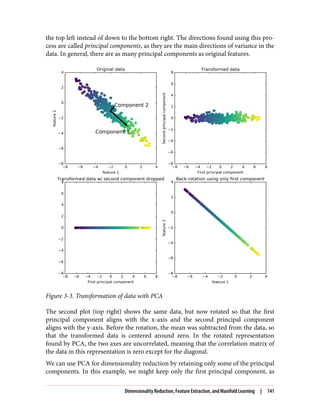
![shown in the third panel in Figure 3-3 (bottom left). This reduces the data from a
two-dimensional dataset to a one-dimensional dataset. Note, however, that instead of
keeping only one of the original features, we found the most interesting direction
(top left to bottom right in the first panel) and kept this direction, the first principal
component.
Finally, we can undo the rotation and add the mean back to the data. This will result
in the data shown in the last panel in Figure 3-3. These points are in the original fea‐
ture space, but we kept only the information contained in the first principal compo‐
nent. This transformation is sometimes used to remove noise effects from the data or
visualize what part of the information is retained using the principal components.
Applying PCA to the cancer dataset for visualization
One of the most common applications of PCA is visualizing high-dimensional data‐
sets. As we saw in Chapter 1, it is hard to create scatter plots of data that has more
than two features. For the Iris dataset, we were able to create a pair plot (Figure 1-3 in
Chapter 1) that gave us a partial picture of the data by showing us all the possible
combinations of two features. But if we want to look at the Breast Cancer dataset,
even using a pair plot is tricky. This dataset has 30 features, which would result in
30 * 14 = 420 scatter plots! We’d never be able to look at all these plots in detail, let
alone try to understand them.
There is an even simpler visualization we can use, though—computing histograms of
each of the features for the two classes, benign and malignant cancer (Figure 3-4):
In[14]:
fig, axes = plt.subplots(15, 2, figsize=(10, 20))
malignant = cancer.data[cancer.target == 0]
benign = cancer.data[cancer.target == 1]
ax = axes.ravel()
for i in range(30):
_, bins = np.histogram(cancer.data[:, i], bins=50)
ax[i].hist(malignant[:, i], bins=bins, color=mglearn.cm3(0), alpha=.5)
ax[i].hist(benign[:, i], bins=bins, color=mglearn.cm3(2), alpha=.5)
ax[i].set_title(cancer.feature_names[i])
ax[i].set_yticks(())
ax[0].set_xlabel("Feature magnitude")
ax[0].set_ylabel("Frequency")
ax[0].legend(["malignant", "benign"], loc="best")
fig.tight_layout()
142 | Chapter 3: Unsupervised Learning and Preprocessing](https://image.slidesharecdn.com/introductiontomachinelearningwithpythonpdfdrive-230107170822-bfb01dbd/85/Introduction-to-Machine-Learning-with-Python-PDFDrive-com-pdf-156-320.jpg)
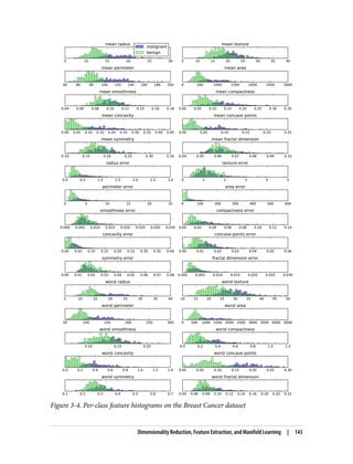
![Here we create a histogram for each of the features, counting how often a data point
appears with a feature in a certain range (called a bin). Each plot overlays two histo‐
grams, one for all of the points in the benign class (blue) and one for all the points in
the malignant class (red). This gives us some idea of how each feature is distributed
across the two classes, and allows us to venture a guess as to which features are better
at distinguishing malignant and benign samples. For example, the feature “smooth‐
ness error” seems quite uninformative, because the two histograms mostly overlap,
while the feature “worst concave points” seems quite informative, because the histo‐
grams are quite disjoint.
However, this plot doesn’t show us anything about the interactions between variables
and how these relate to the classes. Using PCA, we can capture the main interactions
and get a slightly more complete picture. We can find the first two principal compo‐
nents, and visualize the data in this new two-dimensional space with a single scatter
plot.
Before we apply PCA, we scale our data so that each feature has unit variance using
StandardScaler:
In[15]:
from sklearn.datasets import load_breast_cancer
cancer = load_breast_cancer()
scaler = StandardScaler()
scaler.fit(cancer.data)
X_scaled = scaler.transform(cancer.data)
Learning the PCA transformation and applying it is as simple as applying a prepro‐
cessing transformation. We instantiate the PCA object, find the principal components
by calling the fit method, and then apply the rotation and dimensionality reduction
by calling transform. By default, PCA only rotates (and shifts) the data, but keeps all
principal components. To reduce the dimensionality of the data, we need to specify
how many components we want to keep when creating the PCA object:
In[16]:
from sklearn.decomposition import PCA
# keep the first two principal components of the data
pca = PCA(n_components=2)
# fit PCA model to breast cancer data
pca.fit(X_scaled)
# transform data onto the first two principal components
X_pca = pca.transform(X_scaled)
print("Original shape: {}".format(str(X_scaled.shape)))
print("Reduced shape: {}".format(str(X_pca.shape)))
144 | Chapter 3: Unsupervised Learning and Preprocessing](https://image.slidesharecdn.com/introductiontomachinelearningwithpythonpdfdrive-230107170822-bfb01dbd/85/Introduction-to-Machine-Learning-with-Python-PDFDrive-com-pdf-158-320.jpg)
![Out[16]:
Original shape: (569, 30)
Reduced shape: (569, 2)
We can now plot the first two principal components (Figure 3-5):
In[17]:
# plot first vs. second principal component, colored by class
plt.figure(figsize=(8, 8))
mglearn.discrete_scatter(X_pca[:, 0], X_pca[:, 1], cancer.target)
plt.legend(cancer.target_names, loc="best")
plt.gca().set_aspect("equal")
plt.xlabel("First principal component")
plt.ylabel("Second principal component")
Figure 3-5. Two-dimensional scatter plot of the Breast Cancer dataset using the first two
principal components
It is important to note that PCA is an unsupervised method, and does not use any class
information when finding the rotation. It simply looks at the correlations in the data.
For the scatter plot shown here, we plotted the first principal component against the
Dimensionality Reduction, Feature Extraction, and Manifold Learning | 145](https://image.slidesharecdn.com/introductiontomachinelearningwithpythonpdfdrive-230107170822-bfb01dbd/85/Introduction-to-Machine-Learning-with-Python-PDFDrive-com-pdf-159-320.jpg)
![second principal component, and then used the class information to color the points.
You can see that the two classes separate quite well in this two-dimensional space.
This leads us to believe that even a linear classifier (that would learn a line in this
space) could do a reasonably good job at distinguishing the two classes. We can also
see that the malignant (red) points are more spread out than the benign (blue) points
—something that we could already see a bit from the histograms in Figure 3-4.
A downside of PCA is that the two axes in the plot are often not very easy to interpret.
The principal components correspond to directions in the original data, so they are
combinations of the original features. However, these combinations are usually very
complex, as we’ll see shortly. The principal components themselves are stored in the
components_ attribute of the PCA object during fitting:
In[18]:
print("PCA component shape: {}".format(pca.components_.shape))
Out[18]:
PCA component shape: (2, 30)
Each row in components_ corresponds to one principal component, and they are sor‐
ted by their importance (the first principal component comes first, etc.). The columns
correspond to the original features attribute of the PCA in this example, “mean
radius,” “mean texture,” and so on. Let’s have a look at the content of components_:
In[19]:
print("PCA components:n{}".format(pca.components_))
Out[19]:
PCA components:
[[ 0.219 0.104 0.228 0.221 0.143 0.239 0.258 0.261 0.138 0.064
0.206 0.017 0.211 0.203 0.015 0.17 0.154 0.183 0.042 0.103
0.228 0.104 0.237 0.225 0.128 0.21 0.229 0.251 0.123 0.132]
[-0.234 -0.06 -0.215 -0.231 0.186 0.152 0.06 -0.035 0.19 0.367
-0.106 0.09 -0.089 -0.152 0.204 0.233 0.197 0.13 0.184 0.28
-0.22 -0.045 -0.2 -0.219 0.172 0.144 0.098 -0.008 0.142 0.275]]
We can also visualize the coefficients using a heat map (Figure 3-6), which might be
easier to understand:
In[20]:
plt.matshow(pca.components_, cmap='viridis')
plt.yticks([0, 1], ["First component", "Second component"])
plt.colorbar()
plt.xticks(range(len(cancer.feature_names)),
cancer.feature_names, rotation=60, ha='left')
plt.xlabel("Feature")
plt.ylabel("Principal components")
146 | Chapter 3: Unsupervised Learning and Preprocessing](https://image.slidesharecdn.com/introductiontomachinelearningwithpythonpdfdrive-230107170822-bfb01dbd/85/Introduction-to-Machine-Learning-with-Python-PDFDrive-com-pdf-160-320.jpg)
![Figure 3-6. Heat map of the first two principal components on the Breast Cancer dataset
You can see that in the first component, all features have the same sign (it’s negative,
but as we mentioned earlier, it doesn’t matter which direction the arrow points in).
That means that there is a general correlation between all features. As one measure‐
ment is high, the others are likely to be high as well. The second component has
mixed signs, and both of the components involve all of the 30 features. This mixing of
all features is what makes explaining the axes in Figure 3-6 so tricky.
Eigenfaces for feature extraction
Another application of PCA that we mentioned earlier is feature extraction. The idea
behind feature extraction is that it is possible to find a representation of your data
that is better suited to analysis than the raw representation you were given. A great
example of an application where feature extraction is helpful is with images. Images
are made up of pixels, usually stored as red, green, and blue (RGB) intensities.
Objects in images are usually made up of thousands of pixels, and only together are
they meaningful.
We will give a very simple application of feature extraction on images using PCA, by
working with face images from the Labeled Faces in the Wild dataset. This dataset
contains face images of celebrities downloaded from the Internet, and it includes
faces of politicians, singers, actors, and athletes from the early 2000s. We use gray‐
scale versions of these images, and scale them down for faster processing. You can see
some of the images in Figure 3-7:
In[21]:
from sklearn.datasets import fetch_lfw_people
people = fetch_lfw_people(min_faces_per_person=20, resize=0.7)
image_shape = people.images[0].shape
fix, axes = plt.subplots(2, 5, figsize=(15, 8),
subplot_kw={'xticks': (), 'yticks': ()})
for target, image, ax in zip(people.target, people.images, axes.ravel()):
ax.imshow(image)
ax.set_title(people.target_names[target])
Dimensionality Reduction, Feature Extraction, and Manifold Learning | 147](https://image.slidesharecdn.com/introductiontomachinelearningwithpythonpdfdrive-230107170822-bfb01dbd/85/Introduction-to-Machine-Learning-with-Python-PDFDrive-com-pdf-161-320.jpg)
![Figure 3-7. Some images from the Labeled Faces in the Wild dataset
There are 3,023 images, each 87×65 pixels large, belonging to 62 different people:
In[22]:
print("people.images.shape: {}".format(people.images.shape))
print("Number of classes: {}".format(len(people.target_names)))
Out[22]:
people.images.shape: (3023, 87, 65)
Number of classes: 62
The dataset is a bit skewed, however, containing a lot of images of George W. Bush
and Colin Powell, as you can see here:
In[23]:
# count how often each target appears
counts = np.bincount(people.target)
# print counts next to target names
for i, (count, name) in enumerate(zip(counts, people.target_names)):
print("{0:25} {1:3}".format(name, count), end=' ')
if (i + 1) % 3 == 0:
print()
148 | Chapter 3: Unsupervised Learning and Preprocessing](https://image.slidesharecdn.com/introductiontomachinelearningwithpythonpdfdrive-230107170822-bfb01dbd/85/Introduction-to-Machine-Learning-with-Python-PDFDrive-com-pdf-162-320.jpg)
![Out[23]:
Alejandro Toledo 39 Alvaro Uribe 35
Amelie Mauresmo 21 Andre Agassi 36
Angelina Jolie 20 Arnold Schwarzenegger 42
Atal Bihari Vajpayee 24 Bill Clinton 29
Carlos Menem 21 Colin Powell 236
David Beckham 31 Donald Rumsfeld 121
George W Bush 530 George Robertson 22
Gerhard Schroeder 109 Gloria Macapagal Arroyo 44
Gray Davis 26 Guillermo Coria 30
Hamid Karzai 22 Hans Blix 39
Hugo Chavez 71 Igor Ivanov 20
[...] [...]
Laura Bush 41 Lindsay Davenport 22
Lleyton Hewitt 41 Luiz Inacio Lula da Silva 48
Mahmoud Abbas 29 Megawati Sukarnoputri 33
Michael Bloomberg 20 Naomi Watts 22
Nestor Kirchner 37 Paul Bremer 20
Pete Sampras 22 Recep Tayyip Erdogan 30
Ricardo Lagos 27 Roh Moo-hyun 32
Rudolph Giuliani 26 Saddam Hussein 23
Serena Williams 52 Silvio Berlusconi 33
Tiger Woods 23 Tom Daschle 25
Tom Ridge 33 Tony Blair 144
Vicente Fox 32 Vladimir Putin 49
Winona Ryder 24
To make the data less skewed, we will only take up to 50 images of each person
(otherwise, the feature extraction would be overwhelmed by the likelihood of George
W. Bush):
In[24]:
mask = np.zeros(people.target.shape, dtype=np.bool)
for target in np.unique(people.target):
mask[np.where(people.target == target)[0][:50]] = 1
X_people = people.data[mask]
y_people = people.target[mask]
# scale the grayscale values to be between 0 and 1
# instead of 0 and 255 for better numeric stability
X_people = X_people / 255.
A common task in face recognition is to ask if a previously unseen face belongs to a
known person from a database. This has applications in photo collection, social
media, and security applications. One way to solve this problem would be to build a
classifier where each person is a separate class. However, there are usually many dif‐
ferent people in face databases, and very few images of the same person (i.e., very few
training examples per class). That makes it hard to train most classifiers. Additionally,
Dimensionality Reduction, Feature Extraction, and Manifold Learning | 149](https://image.slidesharecdn.com/introductiontomachinelearningwithpythonpdfdrive-230107170822-bfb01dbd/85/Introduction-to-Machine-Learning-with-Python-PDFDrive-com-pdf-163-320.jpg)
![you often want to be able to add new people easily, without needing to retrain a large
model.
A simple solution is to use a one-nearest-neighbor classifier that looks for the most
similar face image to the face you are classifying. This classifier could in principle
work with only a single training example per class. Let’s take a look at how well
KNeighborsClassifier does here:
In[25]:
from sklearn.neighbors import KNeighborsClassifier
# split the data into training and test sets
X_train, X_test, y_train, y_test = train_test_split(
X_people, y_people, stratify=y_people, random_state=0)
# build a KNeighborsClassifier using one neighbor
knn = KNeighborsClassifier(n_neighbors=1)
knn.fit(X_train, y_train)
print("Test set score of 1-nn: {:.2f}".format(knn.score(X_test, y_test)))
Out[25]:
Test set score of 1-nn: 0.27
We obtain an accuracy of 26.6%, which is not actually that bad for a 62-class classifi‐
cation problem (random guessing would give you around 1/62 = 1.5% accuracy), but
is also not great. We only correctly identify a person every fourth time.
This is where PCA comes in. Computing distances in the original pixel space is quite
a bad way to measure similarity between faces. When using a pixel representation to
compare two images, we compare the grayscale value of each individual pixel to the
value of the pixel in the corresponding position in the other image. This representa‐
tion is quite different from how humans would interpret the image of a face, and it is
hard to capture the facial features using this raw representation. For example, using
pixel distances means that shifting a face by one pixel to the right corresponds to a
drastic change, with a completely different representation. We hope that using distan‐
ces along principal components can improve our accuracy. Here, we enable the
whitening option of PCA, which rescales the principal components to have the same
scale. This is the same as using StandardScaler after the transformation. Reusing the
data from Figure 3-3 again, whitening corresponds to not only rotating the data, but
also rescaling it so that the center panel is a circle instead of an ellipse (see
Figure 3-8):
In[26]:
mglearn.plots.plot_pca_whitening()
150 | Chapter 3: Unsupervised Learning and Preprocessing](https://image.slidesharecdn.com/introductiontomachinelearningwithpythonpdfdrive-230107170822-bfb01dbd/85/Introduction-to-Machine-Learning-with-Python-PDFDrive-com-pdf-164-320.jpg)
![Figure 3-8. Transformation of data with PCA using whitening
We fit the PCA object to the training data and extract the first 100 principal compo‐
nents. Then we transform the training and test data:
In[27]:
pca = PCA(n_components=100, whiten=True, random_state=0).fit(X_train)
X_train_pca = pca.transform(X_train)
X_test_pca = pca.transform(X_test)
print("X_train_pca.shape: {}".format(X_train_pca.shape))
Out[27]:
X_train_pca.shape: (1537, 100)
The new data has 100 features, the first 100 principal components. Now, we can use
the new representation to classify our images using a one-nearest-neighbors classifier:
In[28]:
knn = KNeighborsClassifier(n_neighbors=1)
knn.fit(X_train_pca, y_train)
print("Test set accuracy: {:.2f}".format(knn.score(X_test_pca, y_test)))
Out[28]:
Test set accuracy: 0.36
Our accuracy improved quite significantly, from 26.6% to 35.7%, confirming our
intuition that the principal components might provide a better representation of the
data.
Dimensionality Reduction, Feature Extraction, and Manifold Learning | 151](https://image.slidesharecdn.com/introductiontomachinelearningwithpythonpdfdrive-230107170822-bfb01dbd/85/Introduction-to-Machine-Learning-with-Python-PDFDrive-com-pdf-165-320.jpg)
![For image data, we can also easily visualize the principal components that are found.
Remember that components correspond to directions in the input space. The input
space here is 50×37-pixel grayscale images, so directions within this space are also
50×37-pixel grayscale images.
Let’s look at the first couple of principal components (Figure 3-9):
In[29]:
print("pca.components_.shape: {}".format(pca.components_.shape))
Out[29]:
pca.components_.shape: (100, 5655)
In[30]:
fix, axes = plt.subplots(3, 5, figsize=(15, 12),
subplot_kw={'xticks': (), 'yticks': ()})
for i, (component, ax) in enumerate(zip(pca.components_, axes.ravel())):
ax.imshow(component.reshape(image_shape),
cmap='viridis')
ax.set_title("{}. component".format((i + 1)))
While we certainly cannot understand all aspects of these components, we can guess
which aspects of the face images some of the components are capturing. The first
component seems to mostly encode the contrast between the face and the back‐
ground, the second component encodes differences in lighting between the right and
the left half of the face, and so on. While this representation is slightly more semantic
than the raw pixel values, it is still quite far from how a human might perceive a face.
As the PCA model is based on pixels, the alignment of the face (the position of eyes,
chin, and nose) and the lighting both have a strong influence on how similar two
images are in their pixel representation. But alignment and lighting are probably not
what a human would perceive first. When asking people to rate similarity of faces,
they are more likely to use attributes like age, gender, facial expression, and hair style,
which are attributes that are hard to infer from the pixel intensities. It’s important to
keep in mind that algorithms often interpret data (particularly visual data, such as
images, which humans are very familiar with) quite differently from how a human
would.
152 | Chapter 3: Unsupervised Learning and Preprocessing](https://image.slidesharecdn.com/introductiontomachinelearningwithpythonpdfdrive-230107170822-bfb01dbd/85/Introduction-to-Machine-Learning-with-Python-PDFDrive-com-pdf-166-320.jpg)
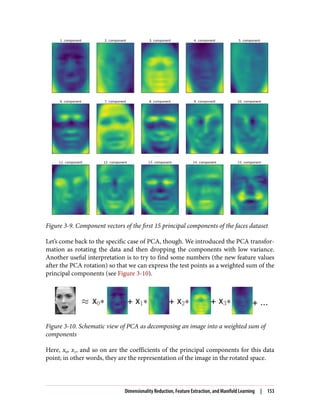
![Another way we can try to understand what a PCA model is doing is by looking at
the reconstructions of the original data using only some components. In Figure 3-3,
after dropping the second component and arriving at the third panel, we undid the
rotation and added the mean back to obtain new points in the original space with the
second component removed, as shown in the last panel. We can do a similar transfor‐
mation for the faces by reducing the data to only some principal components and
then rotating back into the original space. This return to the original feature space
can be done using the inverse_transform method. Here, we visualize the recon‐
struction of some faces using 10, 50, 100, 500, or 2,000 components (Figure 3-11):
In[32]:
mglearn.plots.plot_pca_faces(X_train, X_test, image_shape)
Figure 3-11. Reconstructing three face images using increasing numbers of principal
components
You can see that when we use only the first 10 principal components, only the essence
of the picture, like the face orientation and lighting, is captured. By using more and
more principal components, more and more details in the image are preserved. This
154 | Chapter 3: Unsupervised Learning and Preprocessing](https://image.slidesharecdn.com/introductiontomachinelearningwithpythonpdfdrive-230107170822-bfb01dbd/85/Introduction-to-Machine-Learning-with-Python-PDFDrive-com-pdf-168-320.jpg)
![corresponds to extending the sum in Figure 3-10 to include more and more terms.
Using as many components as there are pixels would mean that we would not discard
any information after the rotation, and we would reconstruct the image perfectly.
We can also try to use PCA to visualize all the faces in the dataset in a scatter plot
using the first two principal components (Figure 3-12), with classes given by who is
shown in the image, similarly to what we did for the cancer dataset:
In[33]:
mglearn.discrete_scatter(X_train_pca[:, 0], X_train_pca[:, 1], y_train)
plt.xlabel("First principal component")
plt.ylabel("Second principal component")
Figure 3-12. Scatter plot of the faces dataset using the first two principal components (see
Figure 3-5 for the corresponding image for the cancer dataset)
As you can see, when we use only the first two principal components the whole data
is just a big blob, with no separation of classes visible. This is not very surprising,
given that even with 10 components, as shown earlier in Figure 3-11, PCA only cap‐
tures very rough characteristics of the faces.
Dimensionality Reduction, Feature Extraction, and Manifold Learning | 155](https://image.slidesharecdn.com/introductiontomachinelearningwithpythonpdfdrive-230107170822-bfb01dbd/85/Introduction-to-Machine-Learning-with-Python-PDFDrive-com-pdf-169-320.jpg)
![Non-Negative Matrix Factorization (NMF)
Non-negative matrix factorization is another unsupervised learning algorithm that
aims to extract useful features. It works similarly to PCA and can also be used for
dimensionality reduction. As in PCA, we are trying to write each data point as a
weighted sum of some components, as illustrated in Figure 3-10. But whereas in PCA
we wanted components that were orthogonal and that explained as much variance of
the data as possible, in NMF, we want the components and the coefficients to be non-
negative; that is, we want both the components and the coefficients to be greater than
or equal to zero. Consequently, this method can only be applied to data where each
feature is non-negative, as a non-negative sum of non-negative components cannot
become negative.
The process of decomposing data into a non-negative weighted sum is particularly
helpful for data that is created as the addition (or overlay) of several independent
sources, such as an audio track of multiple people speaking, or music with many
instruments. In these situations, NMF can identify the original components that
make up the combined data. Overall, NMF leads to more interpretable components
than PCA, as negative components and coefficients can lead to hard-to-interpret can‐
cellation effects. The eigenfaces in Figure 3-9, for example, contain both positive and
negative parts, and as we mentioned in the description of PCA, the sign is actually
arbitrary. Before we apply NMF to the face dataset, let’s briefly revisit the synthetic
data.
Applying NMF to synthetic data
In contrast to when using PCA, we need to ensure that our data is positive for NMF
to be able to operate on the data. This means where the data lies relative to the origin
(0, 0) actually matters for NMF. Therefore, you can think of the non-negative compo‐
nents that are extracted as directions from (0, 0) toward the data.
The following example (Figure 3-13) shows the results of NMF on the two-
dimensional toy data:
In[34]:
mglearn.plots.plot_nmf_illustration()
156 | Chapter 3: Unsupervised Learning and Preprocessing](https://image.slidesharecdn.com/introductiontomachinelearningwithpythonpdfdrive-230107170822-bfb01dbd/85/Introduction-to-Machine-Learning-with-Python-PDFDrive-com-pdf-170-320.jpg)
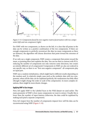
![In[35]:
mglearn.plots.plot_nmf_faces(X_train, X_test, image_shape)
Figure 3-14. Reconstructing three face images using increasing numbers of components
found by NMF
The quality of the back-transformed data is similar to when using PCA, but slightly
worse. This is expected, as PCA finds the optimum directions in terms of reconstruc‐
tion. NMF is usually not used for its ability to reconstruct or encode data, but rather
for finding interesting patterns within the data.
As a first look into the data, let’s try extracting only a few components (say, 15).
Figure 3-15 shows the result:
158 | Chapter 3: Unsupervised Learning and Preprocessing](https://image.slidesharecdn.com/introductiontomachinelearningwithpythonpdfdrive-230107170822-bfb01dbd/85/Introduction-to-Machine-Learning-with-Python-PDFDrive-com-pdf-172-320.jpg)
![In[36]:
from sklearn.decomposition import NMF
nmf = NMF(n_components=15, random_state=0)
nmf.fit(X_train)
X_train_nmf = nmf.transform(X_train)
X_test_nmf = nmf.transform(X_test)
fix, axes = plt.subplots(3, 5, figsize=(15, 12),
subplot_kw={'xticks': (), 'yticks': ()})
for i, (component, ax) in enumerate(zip(nmf.components_, axes.ravel())):
ax.imshow(component.reshape(image_shape))
ax.set_title("{}. component".format(i))
Figure 3-15. The components found by NMF on the faces dataset when using 15 compo‐
nents
These components are all positive, and so resemble prototypes of faces much more so
than the components shown for PCA in Figure 3-9. For example, one can clearly see
that component 3 shows a face rotated somewhat to the right, while component 7
shows a face somewhat rotated to the left. Let’s look at the images for which these
components are particularly strong, shown in Figures 3-16 and 3-17:
Dimensionality Reduction, Feature Extraction, and Manifold Learning | 159](https://image.slidesharecdn.com/introductiontomachinelearningwithpythonpdfdrive-230107170822-bfb01dbd/85/Introduction-to-Machine-Learning-with-Python-PDFDrive-com-pdf-173-320.jpg)
![In[37]:
compn = 3
# sort by 3rd component, plot first 10 images
inds = np.argsort(X_train_nmf[:, compn])[::-1]
fig, axes = plt.subplots(2, 5, figsize=(15, 8),
subplot_kw={'xticks': (), 'yticks': ()})
for i, (ind, ax) in enumerate(zip(inds, axes.ravel())):
ax.imshow(X_train[ind].reshape(image_shape))
compn = 7
# sort by 7th component, plot first 10 images
inds = np.argsort(X_train_nmf[:, compn])[::-1]
fig, axes = plt.subplots(2, 5, figsize=(15, 8),
subplot_kw={'xticks': (), 'yticks': ()})
for i, (ind, ax) in enumerate(zip(inds, axes.ravel())):
ax.imshow(X_train[ind].reshape(image_shape))
Figure 3-16. Faces that have a large coefficient for component 3
160 | Chapter 3: Unsupervised Learning and Preprocessing](https://image.slidesharecdn.com/introductiontomachinelearningwithpythonpdfdrive-230107170822-bfb01dbd/85/Introduction-to-Machine-Learning-with-Python-PDFDrive-com-pdf-174-320.jpg)
![Figure 3-17. Faces that have a large coefficient for component 7
As expected, faces that have a high coefficient for component 3 are faces looking to
the right (Figure 3-16), while faces with a high coefficient for component 7 are look‐
ing to the left (Figure 3-17). As mentioned earlier, extracting patterns like these works
best for data with additive structure, including audio, gene expression, and text data.
Let’s walk through one example on synthetic data to see what this might look like.
Let’s say we are interested in a signal that is a combination of three different sources
(Figure 3-18):
In[38]:
S = mglearn.datasets.make_signals()
plt.figure(figsize=(6, 1))
plt.plot(S, '-')
plt.xlabel("Time")
plt.ylabel("Signal")
Figure 3-18. Original signal sources
Dimensionality Reduction, Feature Extraction, and Manifold Learning | 161](https://image.slidesharecdn.com/introductiontomachinelearningwithpythonpdfdrive-230107170822-bfb01dbd/85/Introduction-to-Machine-Learning-with-Python-PDFDrive-com-pdf-175-320.jpg)
![Unfortunately we cannot observe the original signals, but only an additive mixture of
all three of them. We want to recover the decomposition of the mixed signal into the
original components. We assume that we have many different ways to observe the
mixture (say 100 measurement devices), each of which provides us with a series of
measurements:
In[39]:
# mix data into a 100-dimensional state
A = np.random.RandomState(0).uniform(size=(100, 3))
X = np.dot(S, A.T)
print("Shape of measurements: {}".format(X.shape))
Out[39]:
Shape of measurements: (2000, 100)
We can use NMF to recover the three signals:
In[40]:
nmf = NMF(n_components=3, random_state=42)
S_ = nmf.fit_transform(X)
print("Recovered signal shape: {}".format(S_.shape))
Out[40]:
Recovered signal shape: (2000, 3)
For comparison, we also apply PCA:
In[41]:
pca = PCA(n_components=3)
H = pca.fit_transform(X)
Figure 3-19 shows the signal activity that was discovered by NMF and PCA:
In[42]:
models = [X, S, S_, H]
names = ['Observations (first three measurements)',
'True sources',
'NMF recovered signals',
'PCA recovered signals']
fig, axes = plt.subplots(4, figsize=(8, 4), gridspec_kw={'hspace': .5},
subplot_kw={'xticks': (), 'yticks': ()})
for model, name, ax in zip(models, names, axes):
ax.set_title(name)
ax.plot(model[:, :3], '-')
162 | Chapter 3: Unsupervised Learning and Preprocessing](https://image.slidesharecdn.com/introductiontomachinelearningwithpythonpdfdrive-230107170822-bfb01dbd/85/Introduction-to-Machine-Learning-with-Python-PDFDrive-com-pdf-176-320.jpg)
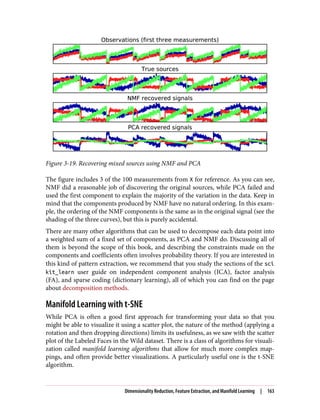
![2 Not to be confused with the much larger MNIST dataset.
Manifold learning algorithms are mainly aimed at visualization, and so are rarely
used to generate more than two new features. Some of them, including t-SNE, com‐
pute a new representation of the training data, but don’t allow transformations of new
data. This means these algorithms cannot be applied to a test set: rather, they can only
transform the data they were trained for. Manifold learning can be useful for explora‐
tory data analysis, but is rarely used if the final goal is supervised learning. The idea
behind t-SNE is to find a two-dimensional representation of the data that preserves
the distances between points as best as possible. t-SNE starts with a random two-
dimensional representation for each data point, and then tries to make points that are
close in the original feature space closer, and points that are far apart in the original
feature space farther apart. t-SNE puts more emphasis on points that are close by,
rather than preserving distances between far-apart points. In other words, it tries to
preserve the information indicating which points are neighbors to each other.
We will apply the t-SNE manifold learning algorithm on a dataset of handwritten dig‐
its that is included in scikit-learn.2
Each data point in this dataset is an 8×8 gray‐
scale image of a handwritten digit between 0 and 1. Figure 3-20 shows an example
image for each class:
In[43]:
from sklearn.datasets import load_digits
digits = load_digits()
fig, axes = plt.subplots(2, 5, figsize=(10, 5),
subplot_kw={'xticks':(), 'yticks': ()})
for ax, img in zip(axes.ravel(), digits.images):
ax.imshow(img)
164 | Chapter 3: Unsupervised Learning and Preprocessing](https://image.slidesharecdn.com/introductiontomachinelearningwithpythonpdfdrive-230107170822-bfb01dbd/85/Introduction-to-Machine-Learning-with-Python-PDFDrive-com-pdf-178-320.jpg)
![Figure 3-20. Example images from the digits dataset
Let’s use PCA to visualize the data reduced to two dimensions. We plot the first two
principal components, and color each dot by its class (see Figure 3-21):
In[44]:
# build a PCA model
pca = PCA(n_components=2)
pca.fit(digits.data)
# transform the digits data onto the first two principal components
digits_pca = pca.transform(digits.data)
colors = ["#476A2A", "#7851B8", "#BD3430", "#4A2D4E", "#875525",
"#A83683", "#4E655E", "#853541", "#3A3120", "#535D8E"]
plt.figure(figsize=(10, 10))
plt.xlim(digits_pca[:, 0].min(), digits_pca[:, 0].max())
plt.ylim(digits_pca[:, 1].min(), digits_pca[:, 1].max())
for i in range(len(digits.data)):
# actually plot the digits as text instead of using scatter
plt.text(digits_pca[i, 0], digits_pca[i, 1], str(digits.target[i]),
color = colors[digits.target[i]],
fontdict={'weight': 'bold', 'size': 9})
plt.xlabel("First principal component")
plt.ylabel("Second principal component")
Here, we actually used the true digit classes as glyphs, to show which class is where.
The digits zero, six, and four are relatively well separated using the first two principal
components, though they still overlap. Most of the other digits overlap significantly.
Dimensionality Reduction, Feature Extraction, and Manifold Learning | 165](https://image.slidesharecdn.com/introductiontomachinelearningwithpythonpdfdrive-230107170822-bfb01dbd/85/Introduction-to-Machine-Learning-with-Python-PDFDrive-com-pdf-179-320.jpg)
![Figure 3-21. Scatter plot of the digits dataset using the first two principal components
Let’s apply t-SNE to the same dataset, and compare the results. As t-SNE does not
support transforming new data, the TSNE class has no transform method. Instead, we
can call the fit_transform method, which will build the model and immediately
return the transformed data (see Figure 3-22):
In[45]:
from sklearn.manifold import TSNE
tsne = TSNE(random_state=42)
# use fit_transform instead of fit, as TSNE has no transform method
digits_tsne = tsne.fit_transform(digits.data)
166 | Chapter 3: Unsupervised Learning and Preprocessing](https://image.slidesharecdn.com/introductiontomachinelearningwithpythonpdfdrive-230107170822-bfb01dbd/85/Introduction-to-Machine-Learning-with-Python-PDFDrive-com-pdf-180-320.jpg)
![In[46]:
plt.figure(figsize=(10, 10))
plt.xlim(digits_tsne[:, 0].min(), digits_tsne[:, 0].max() + 1)
plt.ylim(digits_tsne[:, 1].min(), digits_tsne[:, 1].max() + 1)
for i in range(len(digits.data)):
# actually plot the digits as text instead of using scatter
plt.text(digits_tsne[i, 0], digits_tsne[i, 1], str(digits.target[i]),
color = colors[digits.target[i]],
fontdict={'weight': 'bold', 'size': 9})
plt.xlabel("t-SNE feature 0")
plt.xlabel("t-SNE feature 1")
Figure 3-22. Scatter plot of the digits dataset using two components found by t-SNE
Dimensionality Reduction, Feature Extraction, and Manifold Learning | 167](https://image.slidesharecdn.com/introductiontomachinelearningwithpythonpdfdrive-230107170822-bfb01dbd/85/Introduction-to-Machine-Learning-with-Python-PDFDrive-com-pdf-181-320.jpg)
![The result of t-SNE is quite remarkable. All the classes are quite clearly separated.
The ones and nines are somewhat split up, but most of the classes form a single dense
group. Keep in mind that this method has no knowledge of the class labels: it is com‐
pletely unsupervised. Still, it can find a representation of the data in two dimensions
that clearly separates the classes, based solely on how close points are in the original
space.
The t-SNE algorithm has some tuning parameters, though it often works well with
the default settings. You can try playing with perplexity and early_exaggeration,
but the effects are usually minor.
Clustering
As we described earlier, clustering is the task of partitioning the dataset into groups,
called clusters. The goal is to split up the data in such a way that points within a single
cluster are very similar and points in different clusters are different. Similarly to clas‐
sification algorithms, clustering algorithms assign (or predict) a number to each data
point, indicating which cluster a particular point belongs to.
k-Means Clustering
k-means clustering is one of the simplest and most commonly used clustering algo‐
rithms. It tries to find cluster centers that are representative of certain regions of the
data. The algorithm alternates between two steps: assigning each data point to the
closest cluster center, and then setting each cluster center as the mean of the data
points that are assigned to it. The algorithm is finished when the assignment of
instances to clusters no longer changes. The following example (Figure 3-23) illus‐
trates the algorithm on a synthetic dataset:
In[47]:
mglearn.plots.plot_kmeans_algorithm()
168 | Chapter 3: Unsupervised Learning and Preprocessing](https://image.slidesharecdn.com/introductiontomachinelearningwithpythonpdfdrive-230107170822-bfb01dbd/85/Introduction-to-Machine-Learning-with-Python-PDFDrive-com-pdf-182-320.jpg)
![Figure 3-23. Input data and three steps of the k-means algorithm
Cluster centers are shown as triangles, while data points are shown as circles. Colors
indicate cluster membership. We specified that we are looking for three clusters, so
the algorithm was initialized by declaring three data points randomly as cluster cen‐
ters (see “Initialization”). Then the iterative algorithm starts. First, each data point is
assigned to the cluster center it is closest to (see “Assign Points (1)”). Next, the cluster
centers are updated to be the mean of the assigned points (see “Recompute Centers
(1)”). Then the process is repeated two more times. After the third iteration, the
assignment of points to cluster centers remained unchanged, so the algorithm stops.
Given new data points, k-means will assign each to the closest cluster center. The next
example (Figure 3-24) shows the boundaries of the cluster centers that were learned
in Figure 3-23:
In[48]:
mglearn.plots.plot_kmeans_boundaries()
Clustering | 169](https://image.slidesharecdn.com/introductiontomachinelearningwithpythonpdfdrive-230107170822-bfb01dbd/85/Introduction-to-Machine-Learning-with-Python-PDFDrive-com-pdf-183-320.jpg)
![3 If you don’t provide n_clusters, it is set to 8 by default. There is no particular reason why you should use this
value.
Figure 3-24. Cluster centers and cluster boundaries found by the k-means algorithm
Applying k-means with scikit-learn is quite straightforward. Here, we apply it to
the synthetic data that we used for the preceding plots. We instantiate the KMeans
class, and set the number of clusters we are looking for.3
Then we call the fit method
with the data:
In[49]:
from sklearn.datasets import make_blobs
from sklearn.cluster import KMeans
# generate synthetic two-dimensional data
X, y = make_blobs(random_state=1)
# build the clustering model
kmeans = KMeans(n_clusters=3)
kmeans.fit(X)
During the algorithm, each training data point in X is assigned a cluster label. You can
find these labels in the kmeans.labels_ attribute:
170 | Chapter 3: Unsupervised Learning and Preprocessing](https://image.slidesharecdn.com/introductiontomachinelearningwithpythonpdfdrive-230107170822-bfb01dbd/85/Introduction-to-Machine-Learning-with-Python-PDFDrive-com-pdf-184-320.jpg)
![In[50]:
print("Cluster memberships:n{}".format(kmeans.labels_))
Out[50]:
Cluster memberships:
[1 2 2 2 0 0 0 2 1 1 2 2 0 1 0 0 0 1 2 2 0 2 0 1 2 0 0 1 1 0 1 1 0 1 2 0 2
2 2 0 0 2 1 2 2 0 1 1 1 1 2 0 0 0 1 0 2 2 1 1 2 0 0 2 2 0 1 0 1 2 2 2 0 1
1 2 0 0 1 2 1 2 2 0 1 1 1 1 2 1 0 1 1 2 2 0 0 1 0 1]
As we asked for three clusters, the clusters are numbered 0 to 2.
You can also assign cluster labels to new points, using the predict method. Each new
point is assigned to the closest cluster center when predicting, but the existing model
is not changed. Running predict on the training set returns the same result as
labels_:
In[51]:
print(kmeans.predict(X))
Out[51]:
[1 2 2 2 0 0 0 2 1 1 2 2 0 1 0 0 0 1 2 2 0 2 0 1 2 0 0 1 1 0 1 1 0 1 2 0 2
2 2 0 0 2 1 2 2 0 1 1 1 1 2 0 0 0 1 0 2 2 1 1 2 0 0 2 2 0 1 0 1 2 2 2 0 1
1 2 0 0 1 2 1 2 2 0 1 1 1 1 2 1 0 1 1 2 2 0 0 1 0 1]
You can see that clustering is somewhat similar to classification, in that each item gets
a label. However, there is no ground truth, and consequently the labels themselves
have no a priori meaning. Let’s go back to the example of clustering face images that
we discussed before. It might be that the cluster 3 found by the algorithm contains
only faces of your friend Bela. You can only know that after you look at the pictures,
though, and the number 3 is arbitrary. The only information the algorithm gives you
is that all faces labeled as 3 are similar.
For the clustering we just computed on the two-dimensional toy dataset, that means
that we should not assign any significance to the fact that one group was labeled 0
and another one was labeled 1. Running the algorithm again might result in a differ‐
ent numbering of clusters because of the random nature of the initialization.
Here is a plot of this data again (Figure 3-25). The cluster centers are stored in the
cluster_centers_ attribute, and we plot them as triangles:
In[52]:
mglearn.discrete_scatter(X[:, 0], X[:, 1], kmeans.labels_, markers='o')
mglearn.discrete_scatter(
kmeans.cluster_centers_[:, 0], kmeans.cluster_centers_[:, 1], [0, 1, 2],
markers='^', markeredgewidth=2)
Clustering | 171](https://image.slidesharecdn.com/introductiontomachinelearningwithpythonpdfdrive-230107170822-bfb01dbd/85/Introduction-to-Machine-Learning-with-Python-PDFDrive-com-pdf-185-320.jpg)
![Figure 3-25. Cluster assignments and cluster centers found by k-means with three
clusters
We can also use more or fewer cluster centers (Figure 3-26):
In[53]:
fig, axes = plt.subplots(1, 2, figsize=(10, 5))
# using two cluster centers:
kmeans = KMeans(n_clusters=2)
kmeans.fit(X)
assignments = kmeans.labels_
mglearn.discrete_scatter(X[:, 0], X[:, 1], assignments, ax=axes[0])
# using five cluster centers:
kmeans = KMeans(n_clusters=5)
kmeans.fit(X)
assignments = kmeans.labels_
mglearn.discrete_scatter(X[:, 0], X[:, 1], assignments, ax=axes[1])
172 | Chapter 3: Unsupervised Learning and Preprocessing](https://image.slidesharecdn.com/introductiontomachinelearningwithpythonpdfdrive-230107170822-bfb01dbd/85/Introduction-to-Machine-Learning-with-Python-PDFDrive-com-pdf-186-320.jpg)
![Figure 3-26. Cluster assignments found by k-means using two clusters (left) and five
clusters (right)
Failure cases of k-means
Even if you know the “right” number of clusters for a given dataset, k-means might
not always be able to recover them. Each cluster is defined solely by its center, which
means that each cluster is a convex shape. As a result of this, k-means can only cap‐
ture relatively simple shapes. k-means also assumes that all clusters have the same
“diameter” in some sense; it always draws the boundary between clusters to be exactly
in the middle between the cluster centers. That can sometimes lead to surprising
results, as shown in Figure 3-27:
In[54]:
X_varied, y_varied = make_blobs(n_samples=200,
cluster_std=[1.0, 2.5, 0.5],
random_state=170)
y_pred = KMeans(n_clusters=3, random_state=0).fit_predict(X_varied)
mglearn.discrete_scatter(X_varied[:, 0], X_varied[:, 1], y_pred)
plt.legend(["cluster 0", "cluster 1", "cluster 2"], loc='best')
plt.xlabel("Feature 0")
plt.ylabel("Feature 1")
Clustering | 173](https://image.slidesharecdn.com/introductiontomachinelearningwithpythonpdfdrive-230107170822-bfb01dbd/85/Introduction-to-Machine-Learning-with-Python-PDFDrive-com-pdf-187-320.jpg)
![Figure 3-27. Cluster assignments found by k-means when clusters have different
densities
One might have expected the dense region in the lower left to be the first cluster, the
dense region in the upper right to be the second, and the less dense region in the cen‐
ter to be the third. Instead, both cluster 0 and cluster 1 have some points that are far
away from all the other points in these clusters that “reach” toward the center.
k-means also assumes that all directions are equally important for each cluster. The
following plot (Figure 3-28) shows a two-dimensional dataset where there are three
clearly separated parts in the data. However, these groups are stretched toward the
diagonal. As k-means only considers the distance to the nearest cluster center, it can’t
handle this kind of data:
In[55]:
# generate some random cluster data
X, y = make_blobs(random_state=170, n_samples=600)
rng = np.random.RandomState(74)
# transform the data to be stretched
transformation = rng.normal(size=(2, 2))
X = np.dot(X, transformation)
174 | Chapter 3: Unsupervised Learning and Preprocessing](https://image.slidesharecdn.com/introductiontomachinelearningwithpythonpdfdrive-230107170822-bfb01dbd/85/Introduction-to-Machine-Learning-with-Python-PDFDrive-com-pdf-188-320.jpg)
![# cluster the data into three clusters
kmeans = KMeans(n_clusters=3)
kmeans.fit(X)
y_pred = kmeans.predict(X)
# plot the cluster assignments and cluster centers
plt.scatter(X[:, 0], X[:, 1], c=y_pred, cmap=mglearn.cm3)
plt.scatter(kmeans.cluster_centers_[:, 0], kmeans.cluster_centers_[:, 1],
marker='^', c=[0, 1, 2], s=100, linewidth=2, cmap=mglearn.cm3)
plt.xlabel("Feature 0")
plt.ylabel("Feature 1")
Figure 3-28. k-means fails to identify nonspherical clusters
k-means also performs poorly if the clusters have more complex shapes, like the
two_moons data we encountered in Chapter 2 (see Figure 3-29):
In[56]:
# generate synthetic two_moons data (with less noise this time)
from sklearn.datasets import make_moons
X, y = make_moons(n_samples=200, noise=0.05, random_state=0)
# cluster the data into two clusters
kmeans = KMeans(n_clusters=2)
kmeans.fit(X)
y_pred = kmeans.predict(X)
Clustering | 175](https://image.slidesharecdn.com/introductiontomachinelearningwithpythonpdfdrive-230107170822-bfb01dbd/85/Introduction-to-Machine-Learning-with-Python-PDFDrive-com-pdf-189-320.jpg)
![# plot the cluster assignments and cluster centers
plt.scatter(X[:, 0], X[:, 1], c=y_pred, cmap=mglearn.cm2, s=60)
plt.scatter(kmeans.cluster_centers_[:, 0], kmeans.cluster_centers_[:, 1],
marker='^', c=[mglearn.cm2(0), mglearn.cm2(1)], s=100, linewidth=2)
plt.xlabel("Feature 0")
plt.ylabel("Feature 1")
Figure 3-29. k-means fails to identify clusters with complex shapes
Here, we would hope that the clustering algorithm can discover the two half-moon
shapes. However, this is not possible using the k-means algorithm.
Vector quantization, or seeing k-means as decomposition
Even though k-means is a clustering algorithm, there are interesting parallels between
k-means and the decomposition methods like PCA and NMF that we discussed ear‐
lier. You might remember that PCA tries to find directions of maximum variance in
the data, while NMF tries to find additive components, which often correspond to
“extremes” or “parts” of the data (see Figure 3-13). Both methods tried to express the
data points as a sum over some components. k-means, on the other hand, tries to rep‐
resent each data point using a cluster center. You can think of that as each point being
represented using only a single component, which is given by the cluster center. This
view of k-means as a decomposition method, where each point is represented using a
single component, is called vector quantization.
176 | Chapter 3: Unsupervised Learning and Preprocessing](https://image.slidesharecdn.com/introductiontomachinelearningwithpythonpdfdrive-230107170822-bfb01dbd/85/Introduction-to-Machine-Learning-with-Python-PDFDrive-com-pdf-190-320.jpg)
![Let’s do a side-by-side comparison of PCA, NMF, and k-means, showing the compo‐
nents extracted (Figure 3-30), as well as reconstructions of faces from the test set
using 100 components (Figure 3-31). For k-means, the reconstruction is the closest
cluster center found on the training set:
In[57]:
X_train, X_test, y_train, y_test = train_test_split(
X_people, y_people, stratify=y_people, random_state=0)
nmf = NMF(n_components=100, random_state=0)
nmf.fit(X_train)
pca = PCA(n_components=100, random_state=0)
pca.fit(X_train)
kmeans = KMeans(n_clusters=100, random_state=0)
kmeans.fit(X_train)
X_reconstructed_pca = pca.inverse_transform(pca.transform(X_test))
X_reconstructed_kmeans = kmeans.cluster_centers_[kmeans.predict(X_test)]
X_reconstructed_nmf = np.dot(nmf.transform(X_test), nmf.components_)
In[58]:
fig, axes = plt.subplots(3, 5, figsize=(8, 8),
subplot_kw={'xticks': (), 'yticks': ()})
fig.suptitle("Extracted Components")
for ax, comp_kmeans, comp_pca, comp_nmf in zip(
axes.T, kmeans.cluster_centers_, pca.components_, nmf.components_):
ax[0].imshow(comp_kmeans.reshape(image_shape))
ax[1].imshow(comp_pca.reshape(image_shape), cmap='viridis')
ax[2].imshow(comp_nmf.reshape(image_shape))
axes[0, 0].set_ylabel("kmeans")
axes[1, 0].set_ylabel("pca")
axes[2, 0].set_ylabel("nmf")
fig, axes = plt.subplots(4, 5, subplot_kw={'xticks': (), 'yticks': ()},
figsize=(8, 8))
fig.suptitle("Reconstructions")
for ax, orig, rec_kmeans, rec_pca, rec_nmf in zip(
axes.T, X_test, X_reconstructed_kmeans, X_reconstructed_pca,
X_reconstructed_nmf):
ax[0].imshow(orig.reshape(image_shape))
ax[1].imshow(rec_kmeans.reshape(image_shape))
ax[2].imshow(rec_pca.reshape(image_shape))
ax[3].imshow(rec_nmf.reshape(image_shape))
axes[0, 0].set_ylabel("original")
axes[1, 0].set_ylabel("kmeans")
axes[2, 0].set_ylabel("pca")
axes[3, 0].set_ylabel("nmf")
Clustering | 177](https://image.slidesharecdn.com/introductiontomachinelearningwithpythonpdfdrive-230107170822-bfb01dbd/85/Introduction-to-Machine-Learning-with-Python-PDFDrive-com-pdf-191-320.jpg)
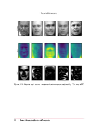
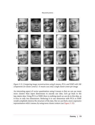
![In[59]:
X, y = make_moons(n_samples=200, noise=0.05, random_state=0)
kmeans = KMeans(n_clusters=10, random_state=0)
kmeans.fit(X)
y_pred = kmeans.predict(X)
plt.scatter(X[:, 0], X[:, 1], c=y_pred, s=60, cmap='Paired')
plt.scatter(kmeans.cluster_centers_[:, 0], kmeans.cluster_centers_[:, 1], s=60,
marker='^', c=range(kmeans.n_clusters), linewidth=2, cmap='Paired')
plt.xlabel("Feature 0")
plt.ylabel("Feature 1")
print("Cluster memberships:n{}".format(y_pred))
Out[59]:
Cluster memberships:
[9 2 5 4 2 7 9 6 9 6 1 0 2 6 1 9 3 0 3 1 7 6 8 6 8 5 2 7 5 8 9 8 6 5 3 7 0
9 4 5 0 1 3 5 2 8 9 1 5 6 1 0 7 4 6 3 3 6 3 8 0 4 2 9 6 4 8 2 8 4 0 4 0 5
6 4 5 9 3 0 7 8 0 7 5 8 9 8 0 7 3 9 7 1 7 2 2 0 4 5 6 7 8 9 4 5 4 1 2 3 1
8 8 4 9 2 3 7 0 9 9 1 5 8 5 1 9 5 6 7 9 1 4 0 6 2 6 4 7 9 5 5 3 8 1 9 5 6
3 5 0 2 9 3 0 8 6 0 3 3 5 6 3 2 0 2 3 0 2 6 3 4 4 1 5 6 7 1 1 3 2 4 7 2 7
3 8 6 4 1 4 3 9 9 5 1 7 5 8 2]
Figure 3-32. Using many k-means clusters to cover the variation in a complex dataset
180 | Chapter 3: Unsupervised Learning and Preprocessing](https://image.slidesharecdn.com/introductiontomachinelearningwithpythonpdfdrive-230107170822-bfb01dbd/85/Introduction-to-Machine-Learning-with-Python-PDFDrive-com-pdf-194-320.jpg)
![4 In this case, “best” means that the sum of variances of the clusters is small.
We used 10 cluster centers, which means each point is now assigned a number
between 0 and 9. We can see this as the data being represented using 10 components
(that is, we have 10 new features), with all features being 0, apart from the one that
represents the cluster center the point is assigned to. Using this 10-dimensional repre‐
sentation, it would now be possible to separate the two half-moon shapes using a lin‐
ear model, which would not have been possible using the original two features. It is
also possible to get an even more expressive representation of the data by using the
distances to each of the cluster centers as features. This can be accomplished using
the transform method of kmeans:
In[60]:
distance_features = kmeans.transform(X)
print("Distance feature shape: {}".format(distance_features.shape))
print("Distance features:n{}".format(distance_features))
Out[60]:
Distance feature shape: (200, 10)
Distance features:
[[ 0.922 1.466 1.14 ..., 1.166 1.039 0.233]
[ 1.142 2.517 0.12 ..., 0.707 2.204 0.983]
[ 0.788 0.774 1.749 ..., 1.971 0.716 0.944]
...,
[ 0.446 1.106 1.49 ..., 1.791 1.032 0.812]
[ 1.39 0.798 1.981 ..., 1.978 0.239 1.058]
[ 1.149 2.454 0.045 ..., 0.572 2.113 0.882]]
k-means is a very popular algorithm for clustering, not only because it is relatively
easy to understand and implement, but also because it runs relatively quickly. k-
means scales easily to large datasets, and scikit-learn even includes a more scalable
variant in the MiniBatchKMeans class, which can handle very large datasets.
One of the drawbacks of k-means is that it relies on a random initialization, which
means the outcome of the algorithm depends on a random seed. By default, scikit-
learn runs the algorithm 10 times with 10 different random initializations, and
returns the best result.4
Further downsides of k-means are the relatively restrictive
assumptions made on the shape of clusters, and the requirement to specify the num‐
ber of clusters you are looking for (which might not be known in a real-world
application).
Next, we will look at two more clustering algorithms that improve upon these proper‐
ties in some ways.
Clustering | 181](https://image.slidesharecdn.com/introductiontomachinelearningwithpythonpdfdrive-230107170822-bfb01dbd/85/Introduction-to-Machine-Learning-with-Python-PDFDrive-com-pdf-195-320.jpg)
![Agglomerative Clustering
Agglomerative clustering refers to a collection of clustering algorithms that all build
upon the same principles: the algorithm starts by declaring each point its own cluster,
and then merges the two most similar clusters until some stopping criterion is satis‐
fied. The stopping criterion implemented in scikit-learn is the number of clusters,
so similar clusters are merged until only the specified number of clusters are left.
There are several linkage criteria that specify how exactly the “most similar cluster” is
measured. This measure is always defined between two existing clusters.
The following three choices are implemented in scikit-learn:
ward
The default choice, ward picks the two clusters to merge such that the variance
within all clusters increases the least. This often leads to clusters that are rela‐
tively equally sized.
average
average linkage merges the two clusters that have the smallest average distance
between all their points.
complete
complete linkage (also known as maximum linkage) merges the two clusters that
have the smallest maximum distance between their points.
ward works on most datasets, and we will use it in our examples. If the clusters have
very dissimilar numbers of members (if one is much bigger than all the others, for
example), average or complete might work better.
The following plot (Figure 3-33) illustrates the progression of agglomerative cluster‐
ing on a two-dimensional dataset, looking for three clusters:
In[61]:
mglearn.plots.plot_agglomerative_algorithm()
182 | Chapter 3: Unsupervised Learning and Preprocessing](https://image.slidesharecdn.com/introductiontomachinelearningwithpythonpdfdrive-230107170822-bfb01dbd/85/Introduction-to-Machine-Learning-with-Python-PDFDrive-com-pdf-196-320.jpg)
![5 We could also use the labels_ attribute, as we did for k-means.
Figure 3-33. Agglomerative clustering iteratively joins the two closest clusters
Initially, each point is its own cluster. Then, in each step, the two clusters that are
closest are merged. In the first four steps, two single-point clusters are picked and
these are joined into two-point clusters. In step 5, one of the two-point clusters is
extended to a third point, and so on. In step 9, there are only three clusters remain‐
ing. As we specified that we are looking for three clusters, the algorithm then stops.
Let’s have a look at how agglomerative clustering performs on the simple three-
cluster data we used here. Because of the way the algorithm works, agglomerative
clustering cannot make predictions for new data points. Therefore, Agglomerative
Clustering has no predict method. To build the model and get the cluster member‐
ships on the training set, use the fit_predict method instead.5
The result is shown
in Figure 3-34:
In[62]:
from sklearn.cluster import AgglomerativeClustering
X, y = make_blobs(random_state=1)
agg = AgglomerativeClustering(n_clusters=3)
assignment = agg.fit_predict(X)
mglearn.discrete_scatter(X[:, 0], X[:, 1], assignment)
plt.xlabel("Feature 0")
plt.ylabel("Feature 1")
Clustering | 183](https://image.slidesharecdn.com/introductiontomachinelearningwithpythonpdfdrive-230107170822-bfb01dbd/85/Introduction-to-Machine-Learning-with-Python-PDFDrive-com-pdf-197-320.jpg)
![Figure 3-34. Cluster assignment using agglomerative clustering with three clusters
As expected, the algorithm recovers the clustering perfectly. While the scikit-learn
implementation of agglomerative clustering requires you to specify the number of
clusters you want the algorithm to find, agglomerative clustering methods provide
some help with choosing the right number, which we will discuss next.
Hierarchical clustering and dendrograms
Agglomerative clustering produces what is known as a hierarchical clustering. The
clustering proceeds iteratively, and every point makes a journey from being a single
point cluster to belonging to some final cluster. Each intermediate step provides a
clustering of the data (with a different number of clusters). It is sometimes helpful to
look at all possible clusterings jointly. The next example (Figure 3-35) shows an over‐
lay of all the possible clusterings shown in Figure 3-33, providing some insight into
how each cluster breaks up into smaller clusters:
In[63]:
mglearn.plots.plot_agglomerative()
184 | Chapter 3: Unsupervised Learning and Preprocessing](https://image.slidesharecdn.com/introductiontomachinelearningwithpythonpdfdrive-230107170822-bfb01dbd/85/Introduction-to-Machine-Learning-with-Python-PDFDrive-com-pdf-198-320.jpg)
![Figure 3-35. Hierarchical cluster assignment (shown as lines) generated with agglomera‐
tive clustering, with numbered data points (cf. Figure 3-36)
While this visualization provides a very detailed view of the hierarchical clustering, it
relies on the two-dimensional nature of the data and therefore cannot be used on
datasets that have more than two features. There is, however, another tool to visualize
hierarchical clustering, called a dendrogram, that can handle multidimensional
datasets.
Unfortunately, scikit-learn currently does not have the functionality to draw den‐
drograms. However, you can generate them easily using SciPy. The SciPy clustering
algorithms have a slightly different interface to the scikit-learn clustering algo‐
rithms. SciPy provides a function that takes a data array X and computes a linkage
array, which encodes hierarchical cluster similarities. We can then feed this linkage
array into the scipy dendrogram function to plot the dendrogram (Figure 3-36):
In[64]:
# Import the dendrogram function and the ward clustering function from SciPy
from scipy.cluster.hierarchy import dendrogram, ward
X, y = make_blobs(random_state=0, n_samples=12)
# Apply the ward clustering to the data array X
# The SciPy ward function returns an array that specifies the distances
# bridged when performing agglomerative clustering
linkage_array = ward(X)
Clustering | 185](https://image.slidesharecdn.com/introductiontomachinelearningwithpythonpdfdrive-230107170822-bfb01dbd/85/Introduction-to-Machine-Learning-with-Python-PDFDrive-com-pdf-199-320.jpg)
![# Now we plot the dendrogram for the linkage_array containing the distances
# between clusters
dendrogram(linkage_array)
# Mark the cuts in the tree that signify two or three clusters
ax = plt.gca()
bounds = ax.get_xbound()
ax.plot(bounds, [7.25, 7.25], '--', c='k')
ax.plot(bounds, [4, 4], '--', c='k')
ax.text(bounds[1], 7.25, ' two clusters', va='center', fontdict={'size': 15})
ax.text(bounds[1], 4, ' three clusters', va='center', fontdict={'size': 15})
plt.xlabel("Sample index")
plt.ylabel("Cluster distance")
Figure 3-36. Dendrogram of the clustering shown in Figure 3-35 with lines indicating
splits into two and three clusters
The dendrogram shows data points as points on the bottom (numbered from 0 to
11). Then, a tree is plotted with these points (representing single-point clusters) as the
leaves, and a new node parent is added for each two clusters that are joined.
Reading from bottom to top, the data points 1 and 4 are joined first (as you could see
in Figure 3-33). Next, points 6 and 9 are joined into a cluster, and so on. At the top
level, there are two branches, one consisting of points 11, 0, 5, 10, 7, 6, and 9, and the
other consisting of points 1, 4, 3, 2, and 8. These correspond to the two largest clus‐
ters in the lefthand side of the plot.
186 | Chapter 3: Unsupervised Learning and Preprocessing](https://image.slidesharecdn.com/introductiontomachinelearningwithpythonpdfdrive-230107170822-bfb01dbd/85/Introduction-to-Machine-Learning-with-Python-PDFDrive-com-pdf-200-320.jpg)
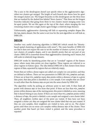
![In the end, there are three kinds of points: core points, points that are within distance
eps of core points (called boundary points), and noise. When the DBSCAN algorithm
is run on a particular dataset multiple times, the clustering of the core points is always
the same, and the same points will always be labeled as noise. However, a boundary
point might be neighbor to core samples of more than one cluster. Therefore, the
cluster membership of boundary points depends on the order in which points are vis‐
ited. Usually there are only few boundary points, and this slight dependence on the
order of points is not important.
Let’s apply DBSCAN on the synthetic dataset we used to demonstrate agglomerative
clustering. Like agglomerative clustering, DBSCAN does not allow predictions on
new test data, so we will use the fit_predict method to perform clustering and
return the cluster labels in one step:
In[65]:
from sklearn.cluster import DBSCAN
X, y = make_blobs(random_state=0, n_samples=12)
dbscan = DBSCAN()
clusters = dbscan.fit_predict(X)
print("Cluster memberships:n{}".format(clusters))
Out[65]:
Cluster memberships:
[-1 -1 -1 -1 -1 -1 -1 -1 -1 -1 -1 -1]
As you can see, all data points were assigned the label -1, which stands for noise. This
is a consequence of the default parameter settings for eps and min_samples, which
are not tuned for small toy datasets. The cluster assignments for different values of
min_samples and eps are shown below, and visualized in Figure 3-37:
In[66]:
mglearn.plots.plot_dbscan()
Out[66]:
min_samples: 2 eps: 1.000000 cluster: [-1 0 0 -1 0 -1 1 1 0 1 -1 -1]
min_samples: 2 eps: 1.500000 cluster: [0 1 1 1 1 0 2 2 1 2 2 0]
min_samples: 2 eps: 2.000000 cluster: [0 1 1 1 1 0 0 0 1 0 0 0]
min_samples: 2 eps: 3.000000 cluster: [0 0 0 0 0 0 0 0 0 0 0 0]
min_samples: 3 eps: 1.000000 cluster: [-1 0 0 -1 0 -1 1 1 0 1 -1 -1]
min_samples: 3 eps: 1.500000 cluster: [0 1 1 1 1 0 2 2 1 2 2 0]
min_samples: 3 eps: 2.000000 cluster: [0 1 1 1 1 0 0 0 1 0 0 0]
min_samples: 3 eps: 3.000000 cluster: [0 0 0 0 0 0 0 0 0 0 0 0]
min_samples: 5 eps: 1.000000 cluster: [-1 -1 -1 -1 -1 -1 -1 -1 -1 -1 -1 -1]
min_samples: 5 eps: 1.500000 cluster: [-1 0 0 0 0 -1 -1 -1 0 -1 -1 -1]
min_samples: 5 eps: 2.000000 cluster: [-1 0 0 0 0 -1 -1 -1 0 -1 -1 -1]
min_samples: 5 eps: 3.000000 cluster: [0 0 0 0 0 0 0 0 0 0 0 0]
188 | Chapter 3: Unsupervised Learning and Preprocessing](https://image.slidesharecdn.com/introductiontomachinelearningwithpythonpdfdrive-230107170822-bfb01dbd/85/Introduction-to-Machine-Learning-with-Python-PDFDrive-com-pdf-202-320.jpg)
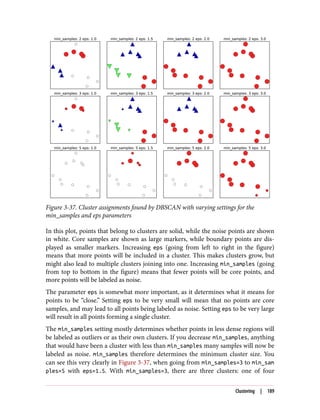
![points, one of five points, and one of three points. Using min_samples=5, the two
smaller clusters (with three and four points) are now labeled as noise, and only the
cluster with five samples remains.
While DBSCAN doesn’t require setting the number of clusters explicitly, setting eps
implicitly controls how many clusters will be found. Finding a good setting for eps is
sometimes easier after scaling the data using StandardScaler or MinMaxScaler, as
using these scaling techniques will ensure that all features have similar ranges.
Figure 3-38 shows the result of running DBSCAN on the two_moons dataset. The
algorithm actually finds the two half-circles and separates them using the default
settings:
In[67]:
X, y = make_moons(n_samples=200, noise=0.05, random_state=0)
# rescale the data to zero mean and unit variance
scaler = StandardScaler()
scaler.fit(X)
X_scaled = scaler.transform(X)
dbscan = DBSCAN()
clusters = dbscan.fit_predict(X_scaled)
# plot the cluster assignments
plt.scatter(X_scaled[:, 0], X_scaled[:, 1], c=clusters, cmap=mglearn.cm2, s=60)
plt.xlabel("Feature 0")
plt.ylabel("Feature 1")
As the algorithm produced the desired number of clusters (two), the parameter set‐
tings seem to work well. If we decrease eps to 0.2 (from the default of 0.5), we will
get eight clusters, which is clearly too many. Increasing eps to 0.7 results in a single
cluster.
When using DBSCAN, you need to be careful about handling the returned cluster
assignments. The use of -1 to indicate noise might result in unexpected effects when
using the cluster labels to index another array.
190 | Chapter 3: Unsupervised Learning and Preprocessing](https://image.slidesharecdn.com/introductiontomachinelearningwithpythonpdfdrive-230107170822-bfb01dbd/85/Introduction-to-Machine-Learning-with-Python-PDFDrive-com-pdf-204-320.jpg)
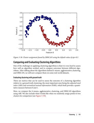
![In[68]:
from sklearn.metrics.cluster import adjusted_rand_score
X, y = make_moons(n_samples=200, noise=0.05, random_state=0)
# rescale the data to zero mean and unit variance
scaler = StandardScaler()
scaler.fit(X)
X_scaled = scaler.transform(X)
fig, axes = plt.subplots(1, 4, figsize=(15, 3),
subplot_kw={'xticks': (), 'yticks': ()})
# make a list of algorithms to use
algorithms = [KMeans(n_clusters=2), AgglomerativeClustering(n_clusters=2),
DBSCAN()]
# create a random cluster assignment for reference
random_state = np.random.RandomState(seed=0)
random_clusters = random_state.randint(low=0, high=2, size=len(X))
# plot random assignment
axes[0].scatter(X_scaled[:, 0], X_scaled[:, 1], c=random_clusters,
cmap=mglearn.cm3, s=60)
axes[0].set_title("Random assignment - ARI: {:.2f}".format(
adjusted_rand_score(y, random_clusters)))
for ax, algorithm in zip(axes[1:], algorithms):
# plot the cluster assignments and cluster centers
clusters = algorithm.fit_predict(X_scaled)
ax.scatter(X_scaled[:, 0], X_scaled[:, 1], c=clusters,
cmap=mglearn.cm3, s=60)
ax.set_title("{} - ARI: {:.2f}".format(algorithm.__class__.__name__,
adjusted_rand_score(y, clusters)))
Figure 3-39. Comparing random assignment, k-means, agglomerative clustering, and
DBSCAN on the two_moons dataset using the supervised ARI score
The adjusted rand index provides intuitive results, with a random cluster assignment
having a score of 0 and DBSCAN (which recovers the desired clustering perfectly)
having a score of 1.
192 | Chapter 3: Unsupervised Learning and Preprocessing](https://image.slidesharecdn.com/introductiontomachinelearningwithpythonpdfdrive-230107170822-bfb01dbd/85/Introduction-to-Machine-Learning-with-Python-PDFDrive-com-pdf-206-320.jpg)
![A common mistake when evaluating clustering in this way is to use accuracy_score
instead of adjusted_rand_score, normalized_mutual_info_score, or some other
clustering metric. The problem in using accuracy is that it requires the assigned clus‐
ter labels to exactly match the ground truth. However, the cluster labels themselves
are meaningless—the only thing that matters is which points are in the same cluster:
In[69]:
from sklearn.metrics import accuracy_score
# these two labelings of points correspond to the same clustering
clusters1 = [0, 0, 1, 1, 0]
clusters2 = [1, 1, 0, 0, 1]
# accuracy is zero, as none of the labels are the same
print("Accuracy: {:.2f}".format(accuracy_score(clusters1, clusters2)))
# adjusted rand score is 1, as the clustering is exactly the same
print("ARI: {:.2f}".format(adjusted_rand_score(clusters1, clusters2)))
Out[69]:
Accuracy: 0.00
ARI: 1.00
Evaluating clustering without ground truth
Although we have just shown one way to evaluate clustering algorithms, in practice,
there is a big problem with using measures like ARI. When applying clustering algo‐
rithms, there is usually no ground truth to which to compare the results. If we knew
the right clustering of the data, we could use this information to build a supervised
model like a classifier. Therefore, using metrics like ARI and NMI usually only helps
in developing algorithms, not in assessing success in an application.
There are scoring metrics for clustering that don’t require ground truth, like the sil‐
houette coefficient. However, these often don’t work well in practice. The silhouette
score computes the compactness of a cluster, where higher is better, with a perfect
score of 1. While compact clusters are good, compactness doesn’t allow for complex
shapes.
Here is an example comparing the outcome of k-means, agglomerative clustering,
and DBSCAN on the two-moons dataset using the silhouette score (Figure 3-40):
In[70]:
from sklearn.metrics.cluster import silhouette_score
X, y = make_moons(n_samples=200, noise=0.05, random_state=0)
# rescale the data to zero mean and unit variance
scaler = StandardScaler()
scaler.fit(X)
X_scaled = scaler.transform(X)
Clustering | 193](https://image.slidesharecdn.com/introductiontomachinelearningwithpythonpdfdrive-230107170822-bfb01dbd/85/Introduction-to-Machine-Learning-with-Python-PDFDrive-com-pdf-207-320.jpg)
![fig, axes = plt.subplots(1, 4, figsize=(15, 3),
subplot_kw={'xticks': (), 'yticks': ()})
# create a random cluster assignment for reference
random_state = np.random.RandomState(seed=0)
random_clusters = random_state.randint(low=0, high=2, size=len(X))
# plot random assignment
axes[0].scatter(X_scaled[:, 0], X_scaled[:, 1], c=random_clusters,
cmap=mglearn.cm3, s=60)
axes[0].set_title("Random assignment: {:.2f}".format(
silhouette_score(X_scaled, random_clusters)))
algorithms = [KMeans(n_clusters=2), AgglomerativeClustering(n_clusters=2),
DBSCAN()]
for ax, algorithm in zip(axes[1:], algorithms):
clusters = algorithm.fit_predict(X_scaled)
# plot the cluster assignments and cluster centers
ax.scatter(X_scaled[:, 0], X_scaled[:, 1], c=clusters, cmap=mglearn.cm3,
s=60)
ax.set_title("{} : {:.2f}".format(algorithm.__class__.__name__,
silhouette_score(X_scaled, clusters)))
Figure 3-40. Comparing random assignment, k-means, agglomerative clustering, and
DBSCAN on the two_moons dataset using the unsupervised silhouette score—the more
intuitive result of DBSCAN has a lower silhouette score than the assignments found by
k-means
As you can see, k-means gets the highest silhouette score, even though we might pre‐
fer the result produced by DBSCAN. A slightly better strategy for evaluating clusters
is using robustness-based clustering metrics. These run an algorithm after adding
some noise to the data, or using different parameter settings, and compare the out‐
comes. The idea is that if many algorithm parameters and many perturbations of the
data return the same result, it is likely to be trustworthy. Unfortunately, this strategy is
not implemented in scikit-learn at the time of writing.
Even if we get a very robust clustering, or a very high silhouette score, we still don’t
know if there is any semantic meaning in the clustering, or whether the clustering
194 | Chapter 3: Unsupervised Learning and Preprocessing](https://image.slidesharecdn.com/introductiontomachinelearningwithpythonpdfdrive-230107170822-bfb01dbd/85/Introduction-to-Machine-Learning-with-Python-PDFDrive-com-pdf-208-320.jpg)
![reflects an aspect of the data that we are interested in. Let’s go back to the example of
face images. We hope to find groups of similar faces—say, men and women, or old
people and young people, or people with beards and without. Let’s say we cluster the
data into two clusters, and all algorithms agree about which points should be clus‐
tered together. We still don’t know if the clusters that are found correspond in any
way to the concepts we are interested in. It could be that they found side views versus
front views, or pictures taken at night versus pictures taken during the day, or pic‐
tures taken with iPhones versus pictures taken with Android phones. The only way to
know whether the clustering corresponds to anything we are interested in is to ana‐
lyze the clusters manually.
Comparing algorithms on the faces dataset
Let’s apply the k-means, DBSCAN, and agglomerative clustering algorithms to the
Labeled Faces in the Wild dataset, and see if any of them find interesting structure.
We will use the eigenface representation of the data, as produced by
PCA(whiten=True), with 100 components:
In[71]:
# extract eigenfaces from lfw data and transform data
from sklearn.decomposition import PCA
pca = PCA(n_components=100, whiten=True, random_state=0)
pca.fit_transform(X_people)
X_pca = pca.transform(X_people)
We saw earlier that this is a more semantic representation of the face images than the
raw pixels. It will also make computation faster. A good exercise would be for you to
run the following experiments on the original data, without PCA, and see if you find
similar clusters.
Analyzing the faces dataset with DBSCAN. We will start by applying DBSCAN, which we
just discussed:
In[72]:
# apply DBSCAN with default parameters
dbscan = DBSCAN()
labels = dbscan.fit_predict(X_pca)
print("Unique labels: {}".format(np.unique(labels)))
Out[72]:
Unique labels: [-1]
We see that all the returned labels are –1, so all of the data was labeled as “noise” by
DBSCAN. There are two things we can change to help this: we can make eps higher,
to expand the neighborhood of each point, and set min_samples lower, to consider
smaller groups of points as clusters. Let’s try changing min_samples first:
Clustering | 195](https://image.slidesharecdn.com/introductiontomachinelearningwithpythonpdfdrive-230107170822-bfb01dbd/85/Introduction-to-Machine-Learning-with-Python-PDFDrive-com-pdf-209-320.jpg)
![In[73]:
dbscan = DBSCAN(min_samples=3)
labels = dbscan.fit_predict(X_pca)
print("Unique labels: {}".format(np.unique(labels)))
Out[73]:
Unique labels: [-1]
Even when considering groups of three points, everything is labeled as noise. So, we
need to increase eps:
In[74]:
dbscan = DBSCAN(min_samples=3, eps=15)
labels = dbscan.fit_predict(X_pca)
print("Unique labels: {}".format(np.unique(labels)))
Out[74]:
Unique labels: [-1 0]
Using a much larger eps of 15, we get only a single cluster and noise points. We can
use this result to find out what the “noise” looks like compared to the rest of the data.
To understand better what’s happening, let’s look at how many points are noise, and
how many points are inside the cluster:
In[75]:
# Count number of points in all clusters and noise.
# bincount doesn't allow negative numbers, so we need to add 1.
# The first number in the result corresponds to noise points.
print("Number of points per cluster: {}".format(np.bincount(labels + 1)))
Out[75]:
Number of points per cluster: [ 27 2036]
There are very few noise points—only 27—so we can look at all of them (see
Figure 3-41):
In[76]:
noise = X_people[labels==-1]
fig, axes = plt.subplots(3, 9, subplot_kw={'xticks': (), 'yticks': ()},
figsize=(12, 4))
for image, ax in zip(noise, axes.ravel()):
ax.imshow(image.reshape(image_shape), vmin=0, vmax=1)
196 | Chapter 3: Unsupervised Learning and Preprocessing](https://image.slidesharecdn.com/introductiontomachinelearningwithpythonpdfdrive-230107170822-bfb01dbd/85/Introduction-to-Machine-Learning-with-Python-PDFDrive-com-pdf-210-320.jpg)
![Figure 3-41. Samples from the faces dataset labeled as noise by DBSCAN
Comparing these images to the random sample of face images from Figure 3-7, we
can guess why they were labeled as noise: the fifth image in the first row shows a per‐
son drinking from a glass, there are images of people wearing hats, and in the last
image there’s a hand in front of the person’s face. The other images contain odd angles
or crops that are too close or too wide.
This kind of analysis—trying to find “the odd one out”—is called outlier detection. If
this was a real application, we might try to do a better job of cropping images, to get
more homogeneous data. There is little we can do about people in photos sometimes
wearing hats, drinking, or holding something in front of their faces, but it’s good to
know that these are issues in the data that any algorithm we might apply needs to
handle.
If we want to find more interesting clusters than just one large one, we need to set eps
smaller, somewhere between 15 and 0.5 (the default). Let’s have a look at what differ‐
ent values of eps result in:
In[77]:
for eps in [1, 3, 5, 7, 9, 11, 13]:
print("neps={}".format(eps))
dbscan = DBSCAN(eps=eps, min_samples=3)
labels = dbscan.fit_predict(X_pca)
print("Clusters present: {}".format(np.unique(labels)))
print("Cluster sizes: {}".format(np.bincount(labels + 1)))
Out[78]:
eps=1
Clusters present: [-1]
Cluster sizes: [2063]
eps=3
Clusters present: [-1]
Cluster sizes: [2063]
Clustering | 197](https://image.slidesharecdn.com/introductiontomachinelearningwithpythonpdfdrive-230107170822-bfb01dbd/85/Introduction-to-Machine-Learning-with-Python-PDFDrive-com-pdf-211-320.jpg)
![eps=5
Clusters present: [-1]
Cluster sizes: [2063]
eps=7
Clusters present: [-1 0 1 2 3 4 5 6 7 8 9 10 11 12]
Cluster sizes: [2006 4 6 6 6 9 3 3 4 3 3 3 3 4]
eps=9
Clusters present: [-1 0 1 2]
Cluster sizes: [1269 788 3 3]
eps=11
Clusters present: [-1 0]
Cluster sizes: [ 430 1633]
eps=13
Clusters present: [-1 0]
Cluster sizes: [ 112 1951]
For low settings of eps, all points are labeled as noise. For eps=7, we get many noise
points and many smaller clusters. For eps=9 we still get many noise points, but we get
one big cluster and some smaller clusters. Starting from eps=11, we get only one large
cluster and noise.
What is interesting to note is that there is never more than one large cluster. At most,
there is one large cluster containing most of the points, and some smaller clusters.
This indicates that there are not two or three different kinds of face images in the data
that are very distinct, but rather that all images are more or less equally similar to (or
dissimilar from) the rest.
The results for eps=7 look most interesting, with many small clusters. We can investi‐
gate this clustering in more detail by visualizing all of the points in each of the 13
small clusters (Figure 3-42):
In[78]:
dbscan = DBSCAN(min_samples=3, eps=7)
labels = dbscan.fit_predict(X_pca)
for cluster in range(max(labels) + 1):
mask = labels == cluster
n_images = np.sum(mask)
fig, axes = plt.subplots(1, n_images, figsize=(n_images * 1.5, 4),
subplot_kw={'xticks': (), 'yticks': ()})
for image, label, ax in zip(X_people[mask], y_people[mask], axes):
ax.imshow(image.reshape(image_shape), vmin=0, vmax=1)
ax.set_title(people.target_names[label].split()[-1])
198 | Chapter 3: Unsupervised Learning and Preprocessing](https://image.slidesharecdn.com/introductiontomachinelearningwithpythonpdfdrive-230107170822-bfb01dbd/85/Introduction-to-Machine-Learning-with-Python-PDFDrive-com-pdf-212-320.jpg)
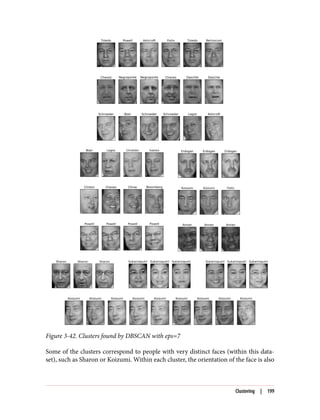
![quite fixed, as well as the facial expression. Some of the clusters contain faces of mul‐
tiple people, but they share a similar orientation and expression.
This concludes our analysis of the DBSCAN algorithm applied to the faces dataset. As
you can see, we are doing a manual analysis here, different from the much more auto‐
matic search approach we could use for supervised learning based on R2
score or
accuracy.
Let’s move on to applying k-means and agglomerative clustering.
Analyzing the faces dataset with k-means. We saw that it was not possible to create
more than one big cluster using DBSCAN. Agglomerative clustering and k-means are
much more likely to create clusters of even size, but we do need to set a target num‐
ber of clusters. We could set the number of clusters to the known number of people in
the dataset, though it is very unlikely that an unsupervised clustering algorithm will
recover them. Instead, we can start with a low number of clusters, like 10, which
might allow us to analyze each of the clusters:
In[79]:
# extract clusters with k-means
km = KMeans(n_clusters=10, random_state=0)
labels_km = km.fit_predict(X_pca)
print("Cluster sizes k-means: {}".format(np.bincount(labels_km)))
Out[79]:
Cluster sizes k-means: [269 128 170 186 386 222 237 64 253 148]
As you can see, k-means clustering partitioned the data into relatively similarly sized
clusters from 64 to 386. This is quite different from the result of DBSCAN.
We can further analyze the outcome of k-means by visualizing the cluster centers
(Figure 3-43). As we clustered in the representation produced by PCA, we need to
rotate the cluster centers back into the original space to visualize them, using
pca.inverse_transform:
In[80]:
fig, axes = plt.subplots(2, 5, subplot_kw={'xticks': (), 'yticks': ()},
figsize=(12, 4))
for center, ax in zip(km.cluster_centers_, axes.ravel()):
ax.imshow(pca.inverse_transform(center).reshape(image_shape),
vmin=0, vmax=1)
200 | Chapter 3: Unsupervised Learning and Preprocessing](https://image.slidesharecdn.com/introductiontomachinelearningwithpythonpdfdrive-230107170822-bfb01dbd/85/Introduction-to-Machine-Learning-with-Python-PDFDrive-com-pdf-214-320.jpg)
![Figure 3-43. Cluster centers found by k-means when setting the number of clusters to 10
The cluster centers found by k-means are very smooth versions of faces. This is not
very surprising, given that each center is an average of 64 to 386 face images. Working
with a reduced PCA representation adds to the smoothness of the images (compared
to the faces reconstructed using 100 PCA dimensions in Figure 3-11). The clustering
seems to pick up on different orientations of the face, different expressions (the third
cluster center seems to show a smiling face), and the presence of shirt collars (see the
second-to-last cluster center).
For a more detailed view, in Figure 3-44 we show for each cluster center the five most
typical images in the cluster (the images assigned to the cluster that are closest to the
cluster center) and the five most atypical images in the cluster (the images assigned to
the cluster that are furthest from the cluster center):
In[81]:
mglearn.plots.plot_kmeans_faces(km, pca, X_pca, X_people,
y_people, people.target_names)
Clustering | 201](https://image.slidesharecdn.com/introductiontomachinelearningwithpythonpdfdrive-230107170822-bfb01dbd/85/Introduction-to-Machine-Learning-with-Python-PDFDrive-com-pdf-215-320.jpg)
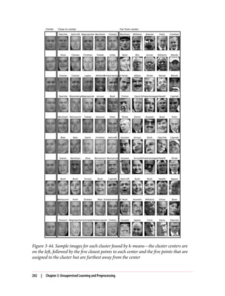
![Figure 3-44 confirms our intuition about smiling faces for the third cluster, and also
the importance of orientation for the other clusters. The “atypical” points are not very
similar to the cluster centers, though, and their assignment seems somewhat arbi‐
trary. This can be attributed to the fact that k-means partitions all the data points and
doesn’t have a concept of “noise” points, as DBSCAN does. Using a larger number of
clusters, the algorithm could find finer distinctions. However, adding more clusters
makes manual inspection even harder.
Analyzing the faces dataset with agglomerative clustering. Now, let’s look at the results of
agglomerative clustering:
In[82]:
# extract clusters with ward agglomerative clustering
agglomerative = AgglomerativeClustering(n_clusters=10)
labels_agg = agglomerative.fit_predict(X_pca)
print("Cluster sizes agglomerative clustering: {}".format(
np.bincount(labels_agg)))
Out[82]:
Cluster sizes agglomerative clustering: [255 623 86 102 122 199 265 26 230 155]
Agglomerative clustering also produces relatively equally sized clusters, with cluster
sizes between 26 and 623. These are more uneven than those produced by k-means,
but much more even than the ones produced by DBSCAN.
We can compute the ARI to measure whether the two partitions of the data given by
agglomerative clustering and k-means are similar:
In[83]:
print("ARI: {:.2f}".format(adjusted_rand_score(labels_agg, labels_km)))
Out[83]:
ARI: 0.13
An ARI of only 0.13 means that the two clusterings labels_agg and labels_km have
little in common. This is not very surprising, given the fact that points further away
from the cluster centers seem to have little in common for k-means.
Next, we might want to plot the dendrogram (Figure 3-45). We’ll limit the depth of
the tree in the plot, as branching down to the individual 2,063 data points would
result in an unreadably dense plot:
Clustering | 203](https://image.slidesharecdn.com/introductiontomachinelearningwithpythonpdfdrive-230107170822-bfb01dbd/85/Introduction-to-Machine-Learning-with-Python-PDFDrive-com-pdf-217-320.jpg)
![In[84]:
linkage_array = ward(X_pca)
# now we plot the dendrogram for the linkage_array
# containing the distances between clusters
plt.figure(figsize=(20, 5))
dendrogram(linkage_array, p=7, truncate_mode='level', no_labels=True)
plt.xlabel("Sample index")
plt.ylabel("Cluster distance")
Figure 3-45. Dendrogram of agglomerative clustering on the faces dataset
Creating 10 clusters, we cut across the tree at the very top, where there are 10 vertical
lines. In the dendrogram for the toy data shown in Figure 3-36, you could see by the
length of the branches that two or three clusters might capture the data appropriately.
For the faces data, there doesn’t seem to be a very natural cutoff point. There are
some branches that represent more distinct groups, but there doesn’t appear to be a
particular number of clusters that is a good fit. This is not surprising, given the results
of DBSCAN, which tried to cluster all points together.
Let’s visualize the 10 clusters, as we did for k-means earlier (Figure 3-46). Note that
there is no notion of cluster center in agglomerative clustering (though we could
compute the mean), and we simply show the first couple of points in each cluster. We
show the number of points in each cluster to the left of the first image:
In[85]:
n_clusters = 10
for cluster in range(n_clusters):
mask = labels_agg == cluster
fig, axes = plt.subplots(1, 10, subplot_kw={'xticks': (), 'yticks': ()},
figsize=(15, 8))
axes[0].set_ylabel(np.sum(mask))
for image, label, asdf, ax in zip(X_people[mask], y_people[mask],
labels_agg[mask], axes):
ax.imshow(image.reshape(image_shape), vmin=0, vmax=1)
ax.set_title(people.target_names[label].split()[-1],
fontdict={'fontsize': 9})
204 | Chapter 3: Unsupervised Learning and Preprocessing](https://image.slidesharecdn.com/introductiontomachinelearningwithpythonpdfdrive-230107170822-bfb01dbd/85/Introduction-to-Machine-Learning-with-Python-PDFDrive-com-pdf-218-320.jpg)
![Figure 3-46. Random images from the clusters generated by In[82]—each row corre‐
sponds to one cluster; the number to the left lists the number of images in each cluster
Clustering | 205](https://image.slidesharecdn.com/introductiontomachinelearningwithpythonpdfdrive-230107170822-bfb01dbd/85/Introduction-to-Machine-Learning-with-Python-PDFDrive-com-pdf-219-320.jpg)
![While some of the clusters seem to have a semantic theme, many of them are too
large to be actually homogeneous. To get more homogeneous clusters, we can run the
algorithm again, this time with 40 clusters, and pick out some of the clusters that are
particularly interesting (Figure 3-47):
In[86]:
# extract clusters with ward agglomerative clustering
agglomerative = AgglomerativeClustering(n_clusters=40)
labels_agg = agglomerative.fit_predict(X_pca)
print("cluster sizes agglomerative clustering: {}".format(np.bincount(labels_agg)))
n_clusters = 40
for cluster in [10, 13, 19, 22, 36]: # hand-picked "interesting" clusters
mask = labels_agg == cluster
fig, axes = plt.subplots(1, 15, subplot_kw={'xticks': (), 'yticks': ()},
figsize=(15, 8))
cluster_size = np.sum(mask)
axes[0].set_ylabel("#{}: {}".format(cluster, cluster_size))
for image, label, asdf, ax in zip(X_people[mask], y_people[mask],
labels_agg[mask], axes):
ax.imshow(image.reshape(image_shape), vmin=0, vmax=1)
ax.set_title(people.target_names[label].split()[-1],
fontdict={'fontsize': 9})
for i in range(cluster_size, 15):
axes[i].set_visible(False)
Out[86]:
cluster sizes agglomerative clustering:
[ 58 80 79 40 222 50 55 78 172 28 26 34 14 11 60 66 152 27
47 31 54 5 8 56 3 5 8 18 22 82 37 89 28 24 41 40
21 10 113 69]
206 | Chapter 3: Unsupervised Learning and Preprocessing](https://image.slidesharecdn.com/introductiontomachinelearningwithpythonpdfdrive-230107170822-bfb01dbd/85/Introduction-to-Machine-Learning-with-Python-PDFDrive-com-pdf-220-320.jpg)
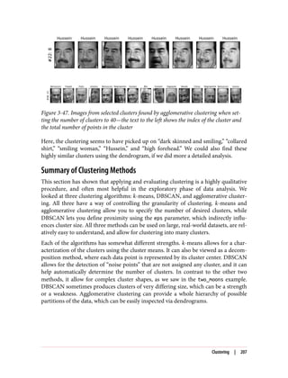
![Summary of the Estimator Interface
Let’s briefly review the API that we introduced in Chapters 2 and 3. All algorithms in
scikit-learn, whether preprocessing, supervised learning, or unsupervised learning
algorithms, are implemented as classes. These classes are called estimators in scikit-
learn. To apply an algorithm, you first have to instantiate an object of the particular
class:
In[87]:
from sklearn.linear_model import LogisticRegression
logreg = LogisticRegression()
The estimator class contains the algorithm, and also stores the model that is learned
from data using the algorithm.
You should set any parameters of the model when constructing the model object.
These parameters include regularization, complexity control, number of clusters to
find, etc. All estimators have a fit method, which is used to build the model. The fit
method always requires as its first argument the data X, represented as a NumPy array
or a SciPy sparse matrix, where each row represents a single data point. The data X is
always assumed to be a NumPy array or SciPy sparse matrix that has continuous
(floating-point) entries. Supervised algorithms also require a y argument, which is a
one-dimensional NumPy array containing target values for regression or classifica‐
tion (i.e., the known output labels or responses).
There are two main ways to apply a learned model in scikit-learn. To create a pre‐
diction in the form of a new output like y, you use the predict method. To create a
new representation of the input data X, you use the transform method. Table 3-1
summarizes the use cases of the predict and transform methods.
Table 3-1. scikit-learn API summary
estimator.fit(x_train, [y_train])
estimator.predict(X_text) estimator.transform(X_test)
Classification Preprocessing
Regression Dimensionality reduction
Clustering Feature extraction
Feature selection
Additionally, all supervised models have a score(X_test, y_test) method that
allows an evaluation of the model. In Table 3-1, X_train and y_train refer to the
training data and training labels, while X_test and y_test refer to the test data and
test labels (if applicable).
Summary and Outlook | 209](https://image.slidesharecdn.com/introductiontomachinelearningwithpythonpdfdrive-230107170822-bfb01dbd/85/Introduction-to-Machine-Learning-with-Python-PDFDrive-com-pdf-223-320.jpg)

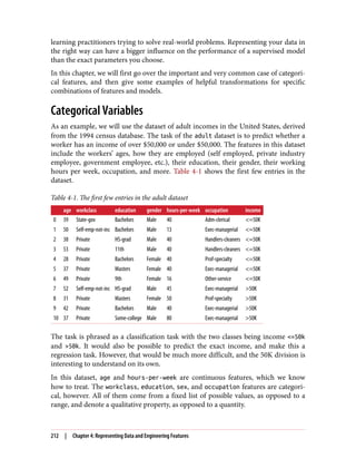
![As a starting point, let’s say we want to learn a logistic regression classifier on this
data. We know from Chapter 2 that a logistic regression makes predictions, ŷ, using
the following formula:
ŷ = w[0] * x[0] + w[1] * x[1] + ... + w[p] * x[p] + b > 0
where w[i] and b are coefficients learned from the training set and x[i] are the input
features. This formula makes sense when x[i] are numbers, but not when x[2] is
"Masters" or "Bachelors". Clearly we need to represent our data in some different
way when applying logistic regression. The next section will explain how we can
overcome this problem.
One-Hot-Encoding (Dummy Variables)
By far the most common way to represent categorical variables is using the one-hot-
encoding or one-out-of-N encoding, also known as dummy variables. The idea behind
dummy variables is to replace a categorical variable with one or more new features
that can have the values 0 and 1. The values 0 and 1 make sense in the formula for
linear binary classification (and for all other models in scikit-learn), and we can
represent any number of categories by introducing one new feature per category, as
described here.
Let’s say for the workclass feature we have possible values of "Government
Employee", "Private Employee", "Self Employed", and "Self Employed Incorpo
rated". To encode these four possible values, we create four new features, called "Gov
ernment Employee", "Private Employee", "Self Employed", and "Self Employed
Incorporated". A feature is 1 if workclass for this person has the corresponding
value and 0 otherwise, so exactly one of the four new features will be 1 for each data
point. This is why this is called one-hot or one-out-of-N encoding.
The principle is illustrated in Table 4-2. A single feature is encoded using four new
features. When using this data in a machine learning algorithm, we would drop the
original workclass feature and only keep the 0–1 features.
Table 4-2. Encoding the workclass feature using one-hot encoding
workclass Government Employee Private Employee Self Employed Self Employed Incorporated
Government Employee 1 0 0 0
Private Employee 0 1 0 0
Self Employed 0 0 1 0
Self Employed Incorporated 0 0 0 1
Categorical Variables | 213](https://image.slidesharecdn.com/introductiontomachinelearningwithpythonpdfdrive-230107170822-bfb01dbd/85/Introduction-to-Machine-Learning-with-Python-PDFDrive-com-pdf-227-320.jpg)
![The one-hot encoding we use is quite similar, but not identical, to
the dummy encoding used in statistics. For simplicity, we encode
each category with a different binary feature. In statistics, it is com‐
mon to encode a categorical feature with k different possible values
into k–1 features (the last one is represented as all zeros). This is
done to simplify the analysis (more technically, this will avoid mak‐
ing the data matrix rank-deficient).
There are two ways to convert your data to a one-hot encoding of categorical vari‐
ables, using either pandas or scikit-learn. At the time of writing, using pandas is
slightly easier, so let’s go this route. First we load the data using pandas from a
comma-separated values (CSV) file:
In[2]:
import pandas as pd
# The file has no headers naming the columns, so we pass header=None
# and provide the column names explicitly in "names"
data = pd.read_csv(
"/home/andy/datasets/adult.data", header=None, index_col=False,
names=['age', 'workclass', 'fnlwgt', 'education', 'education-num',
'marital-status', 'occupation', 'relationship', 'race', 'gender',
'capital-gain', 'capital-loss', 'hours-per-week', 'native-country',
'income'])
# For illustration purposes, we only select some of the columns
data = data[['age', 'workclass', 'education', 'gender', 'hours-per-week',
'occupation', 'income']]
# IPython.display allows nice output formatting within the Jupyter notebook
display(data.head())
Table 4-3 shows the result.
Table 4-3. The first five rows of the adult dataset
age workclass education gender hours-per-week occupation income
0 39 State-gov Bachelors Male 40 Adm-clerical <=50K
1 50 Self-emp-not-inc Bachelors Male 13 Exec-managerial <=50K
2 38 Private HS-grad Male 40 Handlers-cleaners <=50K
3 53 Private 11th Male 40 Handlers-cleaners <=50K
4 28 Private Bachelors Female 40 Prof-specialty <=50K
Checking string-encoded categorical data
After reading a dataset like this, it is often good to first check if a column actually
contains meaningful categorical data. When working with data that was input by
humans (say, users on a website), there might not be a fixed set of categories, and dif‐
ferences in spelling and capitalization might require preprocessing. For example, it
might be that some people specified gender as “male” and some as “man,” and we
214 | Chapter 4: Representing Data and Engineering Features](https://image.slidesharecdn.com/introductiontomachinelearningwithpythonpdfdrive-230107170822-bfb01dbd/85/Introduction-to-Machine-Learning-with-Python-PDFDrive-com-pdf-228-320.jpg)
![might want to represent these two inputs using the same category. A good way to
check the contents of a column is using the value_counts function of a pandas
Series (the type of a single column in a DataFrame), to show us what the unique val‐
ues are and how often they appear:
In[3]:
print(data.gender.value_counts())
Out[3]:
Male 21790
Female 10771
Name: gender, dtype: int64
We can see that there are exactly two values for gender in this dataset, Male and
Female, meaning the data is already in a good format to be represented using one-
hot-encoding. In a real application, you should look at all columns and check their
values. We will skip this here for brevity’s sake.
There is a very simple way to encode the data in pandas, using the get_dummies func‐
tion. The get_dummies function automatically transforms all columns that have
object type (like strings) or are categorical (which is a special pandas concept that we
haven’t talked about yet):
In[4]:
print("Original features:n", list(data.columns), "n")
data_dummies = pd.get_dummies(data)
print("Features after get_dummies:n", list(data_dummies.columns))
Out[4]:
Original features:
['age', 'workclass', 'education', 'gender', 'hours-per-week', 'occupation',
'income']
Features after get_dummies:
['age', 'hours-per-week', 'workclass_ ?', 'workclass_ Federal-gov',
'workclass_ Local-gov', 'workclass_ Never-worked', 'workclass_ Private',
'workclass_ Self-emp-inc', 'workclass_ Self-emp-not-inc',
'workclass_ State-gov', 'workclass_ Without-pay', 'education_ 10th',
'education_ 11th', 'education_ 12th', 'education_ 1st-4th',
...
'education_ Preschool', 'education_ Prof-school', 'education_ Some-college',
'gender_ Female', 'gender_ Male', 'occupation_ ?',
'occupation_ Adm-clerical', 'occupation_ Armed-Forces',
'occupation_ Craft-repair', 'occupation_ Exec-managerial',
'occupation_ Farming-fishing', 'occupation_ Handlers-cleaners',
...
'occupation_ Tech-support', 'occupation_ Transport-moving',
'income_ <=50K', 'income_ >50K']
Categorical Variables | 215](https://image.slidesharecdn.com/introductiontomachinelearningwithpythonpdfdrive-230107170822-bfb01dbd/85/Introduction-to-Machine-Learning-with-Python-PDFDrive-com-pdf-229-320.jpg)
![You can see that the continuous features age and hours-per-week were not touched,
while the categorical features were expanded into one new feature for each possible
value:
In[5]:
data_dummies.head()
Out[5]:
age hours-
per-
week
workclass_ ? workclass_
Federal-
gov
workclass_
Local-gov
… occupation_
Tech-
support
occupation_
Transport-
moving
income_
<=50K
income_
>50K
0 39 40 0.0 0.0 0.0 … 0.0 0.0 1.0 0.0
1 50 13 0.0 0.0 0.0 … 0.0 0.0 1.0 0.0
2 38 40 0.0 0.0 0.0 … 0.0 0.0 1.0 0.0
3 53 40 0.0 0.0 0.0 … 0.0 0.0 1.0 0.0
4 28 40 0.0 0.0 0.0 … 0.0 0.0 1.0 0.0
5 rows × 46 columns
We can now use the values attribute to convert the data_dummies DataFrame into a
NumPy array, and then train a machine learning model on it. Be careful to separate
the target variable (which is now encoded in two income columns) from the data
before training a model. Including the output variable, or some derived property of
the output variable, into the feature representation is a very common mistake in
building supervised machine learning models.
Be careful: column indexing in pandas includes the end of the
range, so 'age':'occupation_ Transport-moving' is inclusive of
occupation_ Transport-moving. This is different from slicing a
NumPy array, where the end of a range is not included: for exam‐
ple, np.arange(11)[0:10] doesn’t include the entry with index 10.
In this case, we extract only the columns containing features—that is, all columns
from age to occupation_ Transport-moving. This range contains all the features but
not the target:
In[6]:
features = data_dummies.ix[:, 'age':'occupation_ Transport-moving']
# Extract NumPy arrays
X = features.values
y = data_dummies['income_ >50K'].values
print("X.shape: {} y.shape: {}".format(X.shape, y.shape))
216 | Chapter 4: Representing Data and Engineering Features](https://image.slidesharecdn.com/introductiontomachinelearningwithpythonpdfdrive-230107170822-bfb01dbd/85/Introduction-to-Machine-Learning-with-Python-PDFDrive-com-pdf-230-320.jpg)
![Out[6]:
X.shape: (32561, 44) y.shape: (32561,)
Now the data is represented in a way that scikit-learn can work with, and we can
proceed as usual:
In[7]:
from sklearn.linear_model import LogisticRegression
from sklearn.model_selection import train_test_split
X_train, X_test, y_train, y_test = train_test_split(X, y, random_state=0)
logreg = LogisticRegression()
logreg.fit(X_train, y_train)
print("Test score: {:.2f}".format(logreg.score(X_test, y_test)))
Out[7]:
Test score: 0.81
In this example, we called get_dummies on a DataFrame containing
both the training and the test data. This is important to ensure cat‐
egorical values are represented in the same way in the training set
and the test set.
Imagine we have the training and test sets in two different Data
Frames. If the "Private Employee" value for the workclass feature
does not appear in the test set, pandas will assume there are only
three possible values for this feature and will create only three new
dummy features. Now our training and test sets have different
numbers of features, and we can’t apply the model we learned on
the training set to the test set anymore. Even worse, imagine the
workclass feature has the values "Government Employee" and
"Private Employee" in the training set, and "Self Employed" and
"Self Employed Incorporated" in the test set. In both cases,
pandas will create two new dummy features, so the encoded Data
Frames will have the same number of features. However, the two
dummy features have entirely different meanings in the training
and test sets. The column that means "Government Employee" for
the training set would encode "Self Employed" for the test set.
If we built a machine learning model on this data it would work
very badly, because it would assume the columns mean the same
things (because they are in the same position) when in fact they
mean very different things. To fix this, either call get_dummies on a
DataFrame that contains both the training and the test data points,
or make sure that the column names are the same for the training
and test sets after calling get_dummies, to ensure they have the
same semantics.
Categorical Variables | 217](https://image.slidesharecdn.com/introductiontomachinelearningwithpythonpdfdrive-230107170822-bfb01dbd/85/Introduction-to-Machine-Learning-with-Python-PDFDrive-com-pdf-231-320.jpg)
![Numbers Can Encode Categoricals
In the example of the adult dataset, the categorical variables were encoded as strings.
On the one hand, that opens up the possibility of spelling errors, but on the other
hand, it clearly marks a variable as categorical. Often, whether for ease of storage or
because of the way the data is collected, categorical variables are encoded as integers.
For example, imagine the census data in the adult dataset was collected using a ques‐
tionnaire, and the answers for workclass were recorded as 0 (first box ticked), 1 (sec‐
ond box ticked), 2 (third box ticked), and so on. Now the column will contain
numbers from 0 to 8, instead of strings like "Private", and it won’t be immediately
obvious to someone looking at the table representing the dataset whether they should
treat this variable as continuous or categorical. Knowing that the numbers indicate
employment status, however, it is clear that these are very distinct states and should
not be modeled by a single continuous variable.
Categorical features are often encoded using integers. That they are
numbers doesn’t mean that they should necessarily be treated as
continuous features. It is not always clear whether an integer fea‐
ture should be treated as continuous or discrete (and one-hot-
encoded). If there is no ordering between the semantics that are
encoded (like in the workclass example), the feature must be
treated as discrete. For other cases, like five-star ratings, the better
encoding depends on the particular task and data and which
machine learning algorithm is used.
The get_dummies function in pandas treats all numbers as continuous and will not
create dummy variables for them. To get around this, you can either use scikit-
learn’s OneHotEncoder, for which you can specify which variables are continuous
and which are discrete, or convert numeric columns in the DataFrame to strings. To
illustrate, let’s create a DataFrame object with two columns, one containing strings
and one containing integers:
In[8]:
# create a DataFrame with an integer feature and a categorical string feature
demo_df = pd.DataFrame({'Integer Feature': [0, 1, 2, 1],
'Categorical Feature': ['socks', 'fox', 'socks', 'box']})
display(demo_df)
Table 4-4 shows the result.
218 | Chapter 4: Representing Data and Engineering Features](https://image.slidesharecdn.com/introductiontomachinelearningwithpythonpdfdrive-230107170822-bfb01dbd/85/Introduction-to-Machine-Learning-with-Python-PDFDrive-com-pdf-232-320.jpg)
![Table 4-4. DataFrame containing categorical string features and integer features
Categorical Feature Integer Feature
0 socks 0
1 fox 1
2 socks 2
3 box 1
Using get_dummies will only encode the string feature and will not change the integer
feature, as you can see in Table 4-5:
In[9]:
pd.get_dummies(demo_df)
Table 4-5. One-hot-encoded version of the data from Table 4-4, leaving the integer feature
unchanged
Integer Feature Categorical Feature_box Categorical Feature_fox Categorical Feature_socks
0 0 0.0 0.0 1.0
1 1 0.0 1.0 0.0
2 2 0.0 0.0 1.0
3 1 1.0 0.0 0.0
If you want dummy variables to be created for the “Integer Feature” column, you can
explicitly list the columns you want to encode using the columns parameter. Then,
both features will be treated as categorical (see Table 4-6):
In[10]:
demo_df['Integer Feature'] = demo_df['Integer Feature'].astype(str)
pd.get_dummies(demo_df, columns=['Integer Feature', 'Categorical Feature'])
Table 4-6. One-hot encoding of the data shown in Table 4-4, encoding the integer and string
features
Integer
Feature_0
Integer
Feature_1
Integer
Feature_2
Categorical
Feature_box
Categorical
Feature_fox
Categorical
Feature_socks
0 1.0 0.0 0.0 0.0 0.0 1.0
1 0.0 1.0 0.0 0.0 1.0 0.0
2 0.0 0.0 1.0 0.0 0.0 1.0
3 0.0 1.0 0.0 1.0 0.0 0.0
Categorical Variables | 219](https://image.slidesharecdn.com/introductiontomachinelearningwithpythonpdfdrive-230107170822-bfb01dbd/85/Introduction-to-Machine-Learning-with-Python-PDFDrive-com-pdf-233-320.jpg)
![Binning, Discretization, Linear Models, and Trees
The best way to represent data depends not only on the semantics of the data, but also
on the kind of model you are using. Linear models and tree-based models (such as
decision trees, gradient boosted trees, and random forests), two large and very com‐
monly used families, have very different properties when it comes to how they work
with different feature representations. Let’s go back to the wave regression dataset that
we used in Chapter 2. It has only a single input feature. Here is a comparison of a
linear regression model and a decision tree regressor on this dataset (see Figure 4-1):
In[11]:
from sklearn.linear_model import LinearRegression
from sklearn.tree import DecisionTreeRegressor
X, y = mglearn.datasets.make_wave(n_samples=100)
line = np.linspace(-3, 3, 1000, endpoint=False).reshape(-1, 1)
reg = DecisionTreeRegressor(min_samples_split=3).fit(X, y)
plt.plot(line, reg.predict(line), label="decision tree")
reg = LinearRegression().fit(X, y)
plt.plot(line, reg.predict(line), label="linear regression")
plt.plot(X[:, 0], y, 'o', c='k')
plt.ylabel("Regression output")
plt.xlabel("Input feature")
plt.legend(loc="best")
As you know, linear models can only model linear relationships, which are lines in
the case of a single feature. The decision tree can build a much more complex model
of the data. However, this is strongly dependent on the representation of the data.
One way to make linear models more powerful on continuous data is to use binning
(also known as discretization) of the feature to split it up into multiple features, as
described here.
220 | Chapter 4: Representing Data and Engineering Features](https://image.slidesharecdn.com/introductiontomachinelearningwithpythonpdfdrive-230107170822-bfb01dbd/85/Introduction-to-Machine-Learning-with-Python-PDFDrive-com-pdf-234-320.jpg)
![Figure 4-1. Comparing linear regression and a decision tree on the wave dataset
We imagine a partition of the input range for the feature (in this case, the numbers
from –3 to 3) into a fixed number of bins—say, 10. A data point will then be repre‐
sented by which bin it falls into. To determine this, we first have to define the bins. In
this case, we’ll define 10 bins equally spaced between –3 and 3. We use the
np.linspace function for this, creating 11 entries, which will create 10 bins—they are
the spaces in between two consecutive boundaries:
In[12]:
bins = np.linspace(-3, 3, 11)
print("bins: {}".format(bins))
Out[12]:
bins: [-3. -2.4 -1.8 -1.2 -0.6 0. 0.6 1.2 1.8 2.4 3. ]
Here, the first bin contains all data points with feature values –3 to –2.68, the second
bin contains all points with feature values from –2.68 to –2.37, and so on.
Next, we record for each data point which bin it falls into. This can be easily compu‐
ted using the np.digitize function:
Binning, Discretization, Linear Models, and Trees | 221](https://image.slidesharecdn.com/introductiontomachinelearningwithpythonpdfdrive-230107170822-bfb01dbd/85/Introduction-to-Machine-Learning-with-Python-PDFDrive-com-pdf-235-320.jpg)
![In[13]:
which_bin = np.digitize(X, bins=bins)
print("nData points:n", X[:5])
print("nBin membership for data points:n", which_bin[:5])
Out[13]:
Data points:
[[-0.753]
[ 2.704]
[ 1.392]
[ 0.592]
[-2.064]]
Bin membership for data points:
[[ 4]
[10]
[ 8]
[ 6]
[ 2]]
What we did here is transform the single continuous input feature in the wave dataset
into a categorical feature that encodes which bin a data point is in. To use a scikit-
learn model on this data, we transform this discrete feature to a one-hot encoding
using the OneHotEncoder from the preprocessing module. The OneHotEncoder does
the same encoding as pandas.get_dummies, though it currently only works on cate‐
gorical variables that are integers:
In[14]:
from sklearn.preprocessing import OneHotEncoder
# transform using the OneHotEncoder
encoder = OneHotEncoder(sparse=False)
# encoder.fit finds the unique values that appear in which_bin
encoder.fit(which_bin)
# transform creates the one-hot encoding
X_binned = encoder.transform(which_bin)
print(X_binned[:5])
Out[14]:
[[ 0. 0. 0. 1. 0. 0. 0. 0. 0. 0.]
[ 0. 0. 0. 0. 0. 0. 0. 0. 0. 1.]
[ 0. 0. 0. 0. 0. 0. 0. 1. 0. 0.]
[ 0. 0. 0. 0. 0. 1. 0. 0. 0. 0.]
[ 0. 1. 0. 0. 0. 0. 0. 0. 0. 0.]]
Because we specified 10 bins, the transformed dataset X_binned now is made up of 10
features:
222 | Chapter 4: Representing Data and Engineering Features](https://image.slidesharecdn.com/introductiontomachinelearningwithpythonpdfdrive-230107170822-bfb01dbd/85/Introduction-to-Machine-Learning-with-Python-PDFDrive-com-pdf-236-320.jpg)
![In[15]:
print("X_binned.shape: {}".format(X_binned.shape))
Out[15]:
X_binned.shape: (100, 10)
Now we build a new linear regression model and a new decision tree model on the
one-hot-encoded data. The result is visualized in Figure 4-2, together with the bin
boundaries, shown as dotted black lines:
In[16]:
line_binned = encoder.transform(np.digitize(line, bins=bins))
reg = LinearRegression().fit(X_binned, y)
plt.plot(line, reg.predict(line_binned), label='linear regression binned')
reg = DecisionTreeRegressor(min_samples_split=3).fit(X_binned, y)
plt.plot(line, reg.predict(line_binned), label='decision tree binned')
plt.plot(X[:, 0], y, 'o', c='k')
plt.vlines(bins, -3, 3, linewidth=1, alpha=.2)
plt.legend(loc="best")
plt.ylabel("Regression output")
plt.xlabel("Input feature")
Figure 4-2. Comparing linear regression and decision tree regression on binned features
Binning, Discretization, Linear Models, and Trees | 223](https://image.slidesharecdn.com/introductiontomachinelearningwithpythonpdfdrive-230107170822-bfb01dbd/85/Introduction-to-Machine-Learning-with-Python-PDFDrive-com-pdf-237-320.jpg)
![The dashed line and solid line are exactly on top of each other, meaning the linear
regression model and the decision tree make exactly the same predictions. For each
bin, they predict a constant value. As features are constant within each bin, any
model must predict the same value for all points within a bin. Comparing what the
models learned before binning the features and after, we see that the linear model
became much more flexible, because it now has a different value for each bin, while
the decision tree model got much less flexible. Binning features generally has no ben‐
eficial effect for tree-based models, as these models can learn to split up the data any‐
where. In a sense, that means decision trees can learn whatever binning is most useful
for predicting on this data. Additionally, decision trees look at multiple features at
once, while binning is usually done on a per-feature basis. However, the linear model
benefited greatly in expressiveness from the transformation of the data.
If there are good reasons to use a linear model for a particular dataset—say, because it
is very large and high-dimensional, but some features have nonlinear relations with
the output—binning can be a great way to increase modeling power.
Interactions and Polynomials
Another way to enrich a feature representation, particularly for linear models, is
adding interaction features and polynomial features of the original data. This kind of
feature engineering is often used in statistical modeling, but it’s also common in many
practical machine learning applications.
As a first example, look again at Figure 4-2. The linear model learned a constant value
for each bin in the wave dataset. We know, however, that linear models can learn not
only offsets, but also slopes. One way to add a slope to the linear model on the binned
data is to add the original feature (the x-axis in the plot) back in. This leads to an 11-
dimensional dataset, as seen in Figure 4-3:
In[17]:
X_combined = np.hstack([X, X_binned])
print(X_combined.shape)
Out[17]:
(100, 11)
In[18]:
reg = LinearRegression().fit(X_combined, y)
line_combined = np.hstack([line, line_binned])
plt.plot(line, reg.predict(line_combined), label='linear regression combined')
for bin in bins:
plt.plot([bin, bin], [-3, 3], ':', c='k')
224 | Chapter 4: Representing Data and Engineering Features](https://image.slidesharecdn.com/introductiontomachinelearningwithpythonpdfdrive-230107170822-bfb01dbd/85/Introduction-to-Machine-Learning-with-Python-PDFDrive-com-pdf-238-320.jpg)
![plt.legend(loc="best")
plt.ylabel("Regression output")
plt.xlabel("Input feature")
plt.plot(X[:, 0], y, 'o', c='k')
Figure 4-3. Linear regression using binned features and a single global slope
In this example, the model learned an offset for each bin, together with a slope. The
learned slope is downward, and shared across all the bins—there is a single x-axis fea‐
ture, which has a single slope. Because the slope is shared across all bins, it doesn’t
seem to be very helpful. We would rather have a separate slope for each bin! We can
achieve this by adding an interaction or product feature that indicates which bin a
data point is in and where it lies on the x-axis. This feature is a product of the bin
indicator and the original feature. Let’s create this dataset:
In[19]:
X_product = np.hstack([X_binned, X * X_binned])
print(X_product.shape)
Out[19]:
(100, 20)
The dataset now has 20 features: the indicators for which bin a data point is in, and a
product of the original feature and the bin indicator. You can think of the product
Interactions and Polynomials | 225](https://image.slidesharecdn.com/introductiontomachinelearningwithpythonpdfdrive-230107170822-bfb01dbd/85/Introduction-to-Machine-Learning-with-Python-PDFDrive-com-pdf-239-320.jpg)
![feature as a separate copy of the x-axis feature for each bin. It is the original feature
within the bin, and zero everywhere else. Figure 4-4 shows the result of the linear
model on this new representation:
In[20]:
reg = LinearRegression().fit(X_product, y)
line_product = np.hstack([line_binned, line * line_binned])
plt.plot(line, reg.predict(line_product), label='linear regression product')
for bin in bins:
plt.plot([bin, bin], [-3, 3], ':', c='k')
plt.plot(X[:, 0], y, 'o', c='k')
plt.ylabel("Regression output")
plt.xlabel("Input feature")
plt.legend(loc="best")
Figure 4-4. Linear regression with a separate slope per bin
As you can see, now each bin has its own offset and slope in this model.
226 | Chapter 4: Representing Data and Engineering Features](https://image.slidesharecdn.com/introductiontomachinelearningwithpythonpdfdrive-230107170822-bfb01dbd/85/Introduction-to-Machine-Learning-with-Python-PDFDrive-com-pdf-240-320.jpg)
![Using binning is one way to expand a continuous feature. Another one is to use poly‐
nomials of the original features. For a given feature x, we might want to consider
x ** 2, x ** 3, x ** 4, and so on. This is implemented in PolynomialFeatures in
the preprocessing module:
In[21]:
from sklearn.preprocessing import PolynomialFeatures
# include polynomials up to x ** 10:
# the default "include_bias=True" adds a feature that's constantly 1
poly = PolynomialFeatures(degree=10, include_bias=False)
poly.fit(X)
X_poly = poly.transform(X)
Using a degree of 10 yields 10 features:
In[22]:
print("X_poly.shape: {}".format(X_poly.shape))
Out[22]:
X_poly.shape: (100, 10)
Let’s compare the entries of X_poly to those of X:
In[23]:
print("Entries of X:n{}".format(X[:5]))
print("Entries of X_poly:n{}".format(X_poly[:5]))
Out[23]:
Entries of X:
[[-0.753]
[ 2.704]
[ 1.392]
[ 0.592]
[-2.064]]
Entries of X_poly:
[[ -0.753 0.567 -0.427 0.321 -0.242 0.182
-0.137 0.103 -0.078 0.058]
[ 2.704 7.313 19.777 53.482 144.632 391.125
1057.714 2860.360 7735.232 20918.278]
[ 1.392 1.938 2.697 3.754 5.226 7.274
10.125 14.094 19.618 27.307]
[ 0.592 0.350 0.207 0.123 0.073 0.043
0.025 0.015 0.009 0.005]
[ -2.064 4.260 -8.791 18.144 -37.448 77.289
-159.516 329.222 -679.478 1402.367]]
You can obtain the semantics of the features by calling the get_feature_names
method, which provides the exponent for each feature:
Interactions and Polynomials | 227](https://image.slidesharecdn.com/introductiontomachinelearningwithpythonpdfdrive-230107170822-bfb01dbd/85/Introduction-to-Machine-Learning-with-Python-PDFDrive-com-pdf-241-320.jpg)
![In[24]:
print("Polynomial feature names:n{}".format(poly.get_feature_names()))
Out[24]:
Polynomial feature names:
['x0', 'x0^2', 'x0^3', 'x0^4', 'x0^5', 'x0^6', 'x0^7', 'x0^8', 'x0^9', 'x0^10']
You can see that the first column of X_poly corresponds exactly to X, while the other
columns are the powers of the first entry. It’s interesting to see how large some of the
values can get. The second column has entries above 20,000, orders of magnitude dif‐
ferent from the rest.
Using polynomial features together with a linear regression model yields the classical
model of polynomial regression (see Figure 4-5):
In[26]:
reg = LinearRegression().fit(X_poly, y)
line_poly = poly.transform(line)
plt.plot(line, reg.predict(line_poly), label='polynomial linear regression')
plt.plot(X[:, 0], y, 'o', c='k')
plt.ylabel("Regression output")
plt.xlabel("Input feature")
plt.legend(loc="best")
Figure 4-5. Linear regression with tenth-degree polynomial features
228 | Chapter 4: Representing Data and Engineering Features](https://image.slidesharecdn.com/introductiontomachinelearningwithpythonpdfdrive-230107170822-bfb01dbd/85/Introduction-to-Machine-Learning-with-Python-PDFDrive-com-pdf-242-320.jpg)
![As you can see, polynomial features yield a very smooth fit on this one-dimensional
data. However, polynomials of high degree tend to behave in extreme ways on the
boundaries or in regions with little data.
As a comparison, here is a kernel SVM model learned on the original data, without
any transformation (see Figure 4-6):
In[26]:
from sklearn.svm import SVR
for gamma in [1, 10]:
svr = SVR(gamma=gamma).fit(X, y)
plt.plot(line, svr.predict(line), label='SVR gamma={}'.format(gamma))
plt.plot(X[:, 0], y, 'o', c='k')
plt.ylabel("Regression output")
plt.xlabel("Input feature")
plt.legend(loc="best")
Figure 4-6. Comparison of different gamma parameters for an SVM with RBF kernel
Using a more complex model, a kernel SVM, we are able to learn a similarly complex
prediction to the polynomial regression without an explicit transformation of the
features.
Interactions and Polynomials | 229](https://image.slidesharecdn.com/introductiontomachinelearningwithpythonpdfdrive-230107170822-bfb01dbd/85/Introduction-to-Machine-Learning-with-Python-PDFDrive-com-pdf-243-320.jpg)
![As a more realistic application of interactions and polynomials, let’s look again at the
Boston Housing dataset. We already used polynomial features on this dataset in
Chapter 2. Now let’s have a look at how these features were constructed, and at how
much the polynomial features help. First we load the data, and rescale it to be
between 0 and 1 using MinMaxScaler:
In[27]:
from sklearn.datasets import load_boston
from sklearn.model_selection import train_test_split
from sklearn.preprocessing import MinMaxScaler
boston = load_boston()
X_train, X_test, y_train, y_test = train_test_split
(boston.data, boston.target, random_state=0)
# rescale data
scaler = MinMaxScaler()
X_train_scaled = scaler.fit_transform(X_train)
X_test_scaled = scaler.transform(X_test)
Now, we extract polynomial features and interactions up to a degree of 2:
In[28]:
poly = PolynomialFeatures(degree=2).fit(X_train_scaled)
X_train_poly = poly.transform(X_train_scaled)
X_test_poly = poly.transform(X_test_scaled)
print("X_train.shape: {}".format(X_train.shape))
print("X_train_poly.shape: {}".format(X_train_poly.shape))
Out[28]:
X_train.shape: (379, 13)
X_train_poly.shape: (379, 105)
The data originally had 13 features, which were expanded into 105 interaction fea‐
tures. These new features represent all possible interactions between two different
original features, as well as the square of each original feature. degree=2 here means
that we look at all features that are the product of up to two original features. The
exact correspondence between input and output features can be found using the
get_feature_names method:
In[29]:
print("Polynomial feature names:n{}".format(poly.get_feature_names()))
Out[29]:
Polynomial feature names:
['1', 'x0', 'x1', 'x2', 'x3', 'x4', 'x5', 'x6', 'x7', 'x8', 'x9', 'x10',
'x11', 'x12', 'x0^2', 'x0 x1', 'x0 x2', 'x0 x3', 'x0 x4', 'x0 x5', 'x0 x6',
'x0 x7', 'x0 x8', 'x0 x9', 'x0 x10', 'x0 x11', 'x0 x12', 'x1^2', 'x1 x2',
230 | Chapter 4: Representing Data and Engineering Features](https://image.slidesharecdn.com/introductiontomachinelearningwithpythonpdfdrive-230107170822-bfb01dbd/85/Introduction-to-Machine-Learning-with-Python-PDFDrive-com-pdf-244-320.jpg)
!['x1 x3', 'x1 x4', 'x1 x5', 'x1 x6', 'x1 x7', 'x1 x8', 'x1 x9', 'x1 x10',
'x1 x11', 'x1 x12', 'x2^2', 'x2 x3', 'x2 x4', 'x2 x5', 'x2 x6', 'x2 x7',
'x2 x8', 'x2 x9', 'x2 x10', 'x2 x11', 'x2 x12', 'x3^2', 'x3 x4', 'x3 x5',
'x3 x6', 'x3 x7', 'x3 x8', 'x3 x9', 'x3 x10', 'x3 x11', 'x3 x12', 'x4^2',
'x4 x5', 'x4 x6', 'x4 x7', 'x4 x8', 'x4 x9', 'x4 x10', 'x4 x11', 'x4 x12',
'x5^2', 'x5 x6', 'x5 x7', 'x5 x8', 'x5 x9', 'x5 x10', 'x5 x11', 'x5 x12',
'x6^2', 'x6 x7', 'x6 x8', 'x6 x9', 'x6 x10', 'x6 x11', 'x6 x12', 'x7^2',
'x7 x8', 'x7 x9', 'x7 x10', 'x7 x11', 'x7 x12', 'x8^2', 'x8 x9', 'x8 x10',
'x8 x11', 'x8 x12', 'x9^2', 'x9 x10', 'x9 x11', 'x9 x12', 'x10^2', 'x10 x11',
'x10 x12', 'x11^2', 'x11 x12', 'x12^2']
The first new feature is a constant feature, called "1" here. The next 13 features are
the original features (called "x0" to "x12"). Then follows the first feature squared
("x0^2") and combinations of the first and the other features.
Let’s compare the performance using Ridge on the data with and without interac‐
tions:
In[30]:
from sklearn.linear_model import Ridge
ridge = Ridge().fit(X_train_scaled, y_train)
print("Score without interactions: {:.3f}".format(
ridge.score(X_test_scaled, y_test)))
ridge = Ridge().fit(X_train_poly, y_train)
print("Score with interactions: {:.3f}".format(
ridge.score(X_test_poly, y_test)))
Out[30]:
Score without interactions: 0.621
Score with interactions: 0.753
Clearly, the interactions and polynomial features gave us a good boost in perfor‐
mance when using Ridge. When using a more complex model like a random forest,
the story is a bit different, though:
In[31]:
from sklearn.ensemble import RandomForestRegressor
rf = RandomForestRegressor(n_estimators=100).fit(X_train_scaled, y_train)
print("Score without interactions: {:.3f}".format(
rf.score(X_test_scaled, y_test)))
rf = RandomForestRegressor(n_estimators=100).fit(X_train_poly, y_train)
print("Score with interactions: {:.3f}".format(rf.score(X_test_poly, y_test)))
Out[31]:
Score without interactions: 0.799
Score with interactions: 0.763
Interactions and Polynomials | 231](https://image.slidesharecdn.com/introductiontomachinelearningwithpythonpdfdrive-230107170822-bfb01dbd/85/Introduction-to-Machine-Learning-with-Python-PDFDrive-com-pdf-245-320.jpg)
![You can see that even without additional features, the random forest beats the
performance of Ridge. Adding interactions and polynomials actually decreases per‐
formance slightly.
Univariate Nonlinear Transformations
We just saw that adding squared or cubed features can help linear models for regres‐
sion. There are other transformations that often prove useful for transforming certain
features: in particular, applying mathematical functions like log, exp, or sin. While
tree-based models only care about the ordering of the features, linear models and
neural networks are very tied to the scale and distribution of each feature, and if there
is a nonlinear relation between the feature and the target, that becomes hard to model
—particularly in regression. The functions log and exp can help by adjusting the rel‐
ative scales in the data so that they can be captured better by a linear model or neural
network. We saw an application of that in Chapter 2 with the memory price data. The
sin and cos functions can come in handy when dealing with data that encodes peri‐
odic patterns.
Most models work best when each feature (and in regression also the target) is loosely
Gaussian distributed—that is, a histogram of each feature should have something
resembling the familiar “bell curve” shape. Using transformations like log and exp is
a hacky but simple and efficient way to achieve this. A particularly common case
when such a transformation can be helpful is when dealing with integer count data.
By count data, we mean features like “how often did user A log in?” Counts are never
negative, and often follow particular statistical patterns. We are using a synthetic
dataset of counts here that has properties similar to those you can find in the wild.
The features are all integer-valued, while the response is continuous:
In[32]:
rnd = np.random.RandomState(0)
X_org = rnd.normal(size=(1000, 3))
w = rnd.normal(size=3)
X = rnd.poisson(10 * np.exp(X_org))
y = np.dot(X_org, w)
Let’s look at the first 10 entries of the first feature. All are integer values and positive,
but apart from that it’s hard to make out a particular pattern.
If we count the appearance of each value, the distribution of values becomes clearer:
232 | Chapter 4: Representing Data and Engineering Features](https://image.slidesharecdn.com/introductiontomachinelearningwithpythonpdfdrive-230107170822-bfb01dbd/85/Introduction-to-Machine-Learning-with-Python-PDFDrive-com-pdf-246-320.jpg)
![In[33]:
print("Number of feature appearances:n{}".format(np.bincount(X[:, 0])))
Out[33]:
Number of feature appearances:
[28 38 68 48 61 59 45 56 37 40 35 34 36 26 23 26 27 21 23 23 18 21 10 9 17
9 7 14 12 7 3 8 4 5 5 3 4 2 4 1 1 3 2 5 3 8 2 5 2 1
2 3 3 2 2 3 3 0 1 2 1 0 0 3 1 0 0 0 1 3 0 1 0 2 0
1 1 0 0 0 0 1 0 0 2 2 0 1 1 0 0 0 0 1 1 0 0 0 0 0
0 0 1 0 0 0 0 0 1 1 0 0 1 0 0 0 0 0 0 0 1 0 0 0 0
1 0 0 0 0 0 0 0 0 0 0 0 0 0 0 1]
The value 2 seems to be the most common, with 62 appearances (bincount always
starts at 0), and the counts for higher values fall quickly. However, there are some
very high values, like 134 appearing twice. We visualize the counts in Figure 4-7:
In[34]:
bins = np.bincount(X[:, 0])
plt.bar(range(len(bins)), bins, color='w')
plt.ylabel("Number of appearances")
plt.xlabel("Value")
Figure 4-7. Histogram of feature values for X[0]
Univariate Nonlinear Transformations | 233](https://image.slidesharecdn.com/introductiontomachinelearningwithpythonpdfdrive-230107170822-bfb01dbd/85/Introduction-to-Machine-Learning-with-Python-PDFDrive-com-pdf-247-320.jpg)
![1 This is a Poisson distribution, which is quite fundamental to count data.
Features X[:, 1] and X[:, 2] have similar properties. This kind of distribution of
values (many small ones and a few very large ones) is very common in practice.1
However, it is something most linear models can’t handle very well. Let’s try to fit a
ridge regression to this model:
In[35]:
from sklearn.linear_model import Ridge
X_train, X_test, y_train, y_test = train_test_split(X, y, random_state=0)
score = Ridge().fit(X_train, y_train).score(X_test, y_test)
print("Test score: {:.3f}".format(score))
Out[35]:
Test score: 0.622
As you can see from the relatively low R2
score, Ridge was not able to really capture
the relationship between X and y. Applying a logarithmic transformation can help,
though. Because the value 0 appears in the data (and the logarithm is not defined at
0), we can’t actually just apply log, but we have to compute log(X + 1):
In[36]:
X_train_log = np.log(X_train + 1)
X_test_log = np.log(X_test + 1)
After the transformation, the distribution of the data is less asymmetrical and doesn’t
have very large outliers anymore (see Figure 4-8):
In[37]:
plt.hist(np.log(X_train_log[:, 0] + 1), bins=25, color='gray')
plt.ylabel("Number of appearances")
plt.xlabel("Value")
234 | Chapter 4: Representing Data and Engineering Features](https://image.slidesharecdn.com/introductiontomachinelearningwithpythonpdfdrive-230107170822-bfb01dbd/85/Introduction-to-Machine-Learning-with-Python-PDFDrive-com-pdf-248-320.jpg)
![2 This is a very crude approximation of using Poisson regression, which would be the proper solution from a
probabilistic standpoint.
Figure 4-8. Histogram of feature values for X[0] after logarithmic transformation
Building a ridge model on the new data provides a much better fit:
In[38]:
score = Ridge().fit(X_train_log, y_train).score(X_test_log, y_test)
print("Test score: {:.3f}".format(score))
Out[38]:
Test score: 0.875
Finding the transformation that works best for each combination of dataset and
model is somewhat of an art. In this example, all the features had the same properties.
This is rarely the case in practice, and usually only a subset of the features should be
transformed, or sometimes each feature needs to be transformed in a different way.
As we mentioned earlier, these kinds of transformations are irrelevant for tree-based
models but might be essential for linear models. Sometimes it is also a good idea to
transform the target variable y in regression. Trying to predict counts (say, number of
orders) is a fairly common task, and using the log(y + 1) transformation often
helps.2
Univariate Nonlinear Transformations | 235](https://image.slidesharecdn.com/introductiontomachinelearningwithpythonpdfdrive-230107170822-bfb01dbd/85/Introduction-to-Machine-Learning-with-Python-PDFDrive-com-pdf-249-320.jpg)
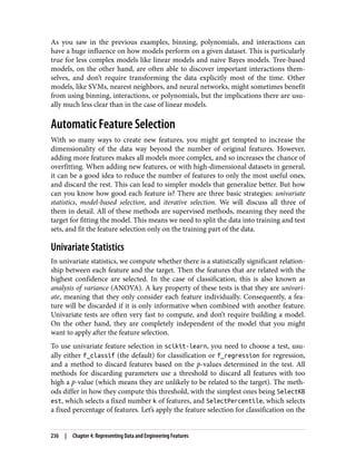
![cancer dataset. To make the task a bit harder, we’ll add some noninformative noise
features to the data. We expect the feature selection to be able to identify the features
that are noninformative and remove them:
In[39]:
from sklearn.datasets import load_breast_cancer
from sklearn.feature_selection import SelectPercentile
from sklearn.model_selection import train_test_split
cancer = load_breast_cancer()
# get deterministic random numbers
rng = np.random.RandomState(42)
noise = rng.normal(size=(len(cancer.data), 50))
# add noise features to the data
# the first 30 features are from the dataset, the next 50 are noise
X_w_noise = np.hstack([cancer.data, noise])
X_train, X_test, y_train, y_test = train_test_split(
X_w_noise, cancer.target, random_state=0, test_size=.5)
# use f_classif (the default) and SelectPercentile to select 50% of features
select = SelectPercentile(percentile=50)
select.fit(X_train, y_train)
# transform training set
X_train_selected = select.transform(X_train)
print("X_train.shape: {}".format(X_train.shape))
print("X_train_selected.shape: {}".format(X_train_selected.shape))
Out[39]:
X_train.shape: (284, 80)
X_train_selected.shape: (284, 40)
As you can see, the number of features was reduced from 80 to 40 (50 percent of the
original number of features). We can find out which features have been selected using
the get_support method, which returns a Boolean mask of the selected features
(visualized in Figure 4-9):
In[40]:
mask = select.get_support()
print(mask)
# visualize the mask -- black is True, white is False
plt.matshow(mask.reshape(1, -1), cmap='gray_r')
plt.xlabel("Sample index")
Out[40]:
[ True True True True True True True True True False True False
True True True True True True False False True True True True
True True True True True True False False False True False True
Automatic Feature Selection | 237](https://image.slidesharecdn.com/introductiontomachinelearningwithpythonpdfdrive-230107170822-bfb01dbd/85/Introduction-to-Machine-Learning-with-Python-PDFDrive-com-pdf-251-320.jpg)
![False False True False False False False True False False True False
False True False True False False False False False False True False
True False False False False True False True False False False False
True True False True False False False False]
Figure 4-9. Features selected by SelectPercentile
As you can see from the visualization of the mask, most of the selected features are
the original features, and most of the noise features were removed. However, the
recovery of the original features is not perfect. Let’s compare the performance of
logistic regression on all features against the performance using only the selected
features:
In[41]:
from sklearn.linear_model import LogisticRegression
# transform test data
X_test_selected = select.transform(X_test)
lr = LogisticRegression()
lr.fit(X_train, y_train)
print("Score with all features: {:.3f}".format(lr.score(X_test, y_test)))
lr.fit(X_train_selected, y_train)
print("Score with only selected features: {:.3f}".format(
lr.score(X_test_selected, y_test)))
Out[41]:
Score with all features: 0.930
Score with only selected features: 0.940
In this case, removing the noise features improved performance, even though some
of the original features were lost. This was a very simple synthetic example, and out‐
comes on real data are usually mixed. Univariate feature selection can still be very
helpful, though, if there is such a large number of features that building a model on
them is infeasible, or if you suspect that many features are completely uninformative.
Model-Based Feature Selection
Model-based feature selection uses a supervised machine learning model to judge the
importance of each feature, and keeps only the most important ones. The supervised
model that is used for feature selection doesn’t need to be the same model that is used
for the final supervised modeling. The feature selection model needs to provide some
measure of importance for each feature, so that they can be ranked by this measure.
Decision trees and decision tree–based models provide a feature_importances_
238 | Chapter 4: Representing Data and Engineering Features](https://image.slidesharecdn.com/introductiontomachinelearningwithpythonpdfdrive-230107170822-bfb01dbd/85/Introduction-to-Machine-Learning-with-Python-PDFDrive-com-pdf-252-320.jpg)
![attribute, which directly encodes the importance of each feature. Linear models have
coefficients, which can also be used to capture feature importances by considering the
absolute values. As we saw in Chapter 2, linear models with L1 penalty learn sparse
coefficients, which only use a small subset of features. This can be viewed as a form of
feature selection for the model itself, but can also be used as a preprocessing step to
select features for another model. In contrast to univariate selection, model-based
selection considers all features at once, and so can capture interactions (if the model
can capture them). To use model-based feature selection, we need to use the
SelectFromModel transformer:
In[42]:
from sklearn.feature_selection import SelectFromModel
from sklearn.ensemble import RandomForestClassifier
select = SelectFromModel(
RandomForestClassifier(n_estimators=100, random_state=42),
threshold="median")
The SelectFromModel class selects all features that have an importance measure of
the feature (as provided by the supervised model) greater than the provided thresh‐
old. To get a comparable result to what we got with univariate feature selection, we
used the median as a threshold, so that half of the features will be selected. We use a
random forest classifier with 100 trees to compute the feature importances. This is a
quite complex model and much more powerful than using univariate tests. Now let’s
actually fit the model:
In[43]:
select.fit(X_train, y_train)
X_train_l1 = select.transform(X_train)
print("X_train.shape: {}".format(X_train.shape))
print("X_train_l1.shape: {}".format(X_train_l1.shape))
Out[43]:
X_train.shape: (284, 80)
X_train_l1.shape: (284, 40)
Again, we can have a look at the features that were selected (Figure 4-10):
In[44]:
mask = select.get_support()
# visualize the mask -- black is True, white is False
plt.matshow(mask.reshape(1, -1), cmap='gray_r')
plt.xlabel("Sample index")
Figure 4-10. Features selected by SelectFromModel using the RandomForestClassifier
Automatic Feature Selection | 239](https://image.slidesharecdn.com/introductiontomachinelearningwithpythonpdfdrive-230107170822-bfb01dbd/85/Introduction-to-Machine-Learning-with-Python-PDFDrive-com-pdf-253-320.jpg)
![This time, all but two of the original features were selected. Because we specified to
select 40 features, some of the noise features are also selected. Let’s take a look at the
performance:
In[45]:
X_test_l1 = select.transform(X_test)
score = LogisticRegression().fit(X_train_l1, y_train).score(X_test_l1, y_test)
print("Test score: {:.3f}".format(score))
Out[45]:
Test score: 0.951
With the better feature selection, we also gained some improvements here.
Iterative Feature Selection
In univariate testing we used no model, while in model-based selection we used a sin‐
gle model to select features. In iterative feature selection, a series of models are built,
with varying numbers of features. There are two basic methods: starting with no fea‐
tures and adding features one by one until some stopping criterion is reached, or
starting with all features and removing features one by one until some stopping crite‐
rion is reached. Because a series of models are built, these methods are much more
computationally expensive than the methods we discussed previously. One particular
method of this kind is recursive feature elimination (RFE), which starts with all fea‐
tures, builds a model, and discards the least important feature according to the
model. Then a new model is built using all but the discarded feature, and so on until
only a prespecified number of features are left. For this to work, the model used for
selection needs to provide some way to determine feature importance, as was the case
for the model-based selection. Here, we use the same random forest model that we
used earlier, and get the results shown in Figure 4-11:
In[46]:
from sklearn.feature_selection import RFE
select = RFE(RandomForestClassifier(n_estimators=100, random_state=42),
n_features_to_select=40)
select.fit(X_train, y_train)
# visualize the selected features:
mask = select.get_support()
plt.matshow(mask.reshape(1, -1), cmap='gray_r')
plt.xlabel("Sample index")
240 | Chapter 4: Representing Data and Engineering Features](https://image.slidesharecdn.com/introductiontomachinelearningwithpythonpdfdrive-230107170822-bfb01dbd/85/Introduction-to-Machine-Learning-with-Python-PDFDrive-com-pdf-254-320.jpg)
![Figure 4-11. Features selected by recursive feature elimination with the random forest
classifier model
The feature selection got better compared to the univariate and model-based selec‐
tion, but one feature was still missed. Running this code also takes significantly longer
than that for the model-based selection, because a random forest model is trained 40
times, once for each feature that is dropped. Let’s test the accuracy of the logistic
regression model when using RFE for feature selection:
In[47]:
X_train_rfe= select.transform(X_train)
X_test_rfe= select.transform(X_test)
score = LogisticRegression().fit(X_train_rfe, y_train).score(X_test_rfe, y_test)
print("Test score: {:.3f}".format(score))
Out[47]:
Test score: 0.951
We can also use the model used inside the RFE to make predictions. This uses only
the feature set that was selected:
In[48]:
print("Test score: {:.3f}".format(select.score(X_test, y_test)))
Out[48]:
Test score: 0.951
Here, the performance of the random forest used inside the RFE is the same as that
achieved by training a logistic regression model on top of the selected features. In
other words, once we’ve selected the right features, the linear model performs as well
as the random forest.
If you are unsure when selecting what to use as input to your machine learning algo‐
rithms, automatic feature selection can be quite helpful. It is also great for reducing
the amount of features needed—for example, to speed up prediction or to allow for
more interpretable models. In most real-world cases, applying feature selection is
unlikely to provide large gains in performance. However, it is still a valuable tool in
the toolbox of the feature engineer.
Automatic Feature Selection | 241](https://image.slidesharecdn.com/introductiontomachinelearningwithpythonpdfdrive-230107170822-bfb01dbd/85/Introduction-to-Machine-Learning-with-Python-PDFDrive-com-pdf-255-320.jpg)
![Utilizing Expert Knowledge
Feature engineering is often an important place to use expert knowledge for a particu‐
lar application. While the purpose of machine learning in many cases is to avoid hav‐
ing to create a set of expert-designed rules, that doesn’t mean that prior knowledge of
the application or domain should be discarded. Often, domain experts can help in
identifying useful features that are much more informative than the initial represen‐
tation of the data. Imagine you work for a travel agency and want to predict flight
prices. Let’s say you have a record of prices together with dates, airlines, start loca‐
tions, and destinations. A machine learning model might be able to build a decent
model from that. Some important factors in flight prices, however, cannot be learned.
For example, flights are usually more expensive during peak vacation months and
around holidays. While the dates of some holidays (like Christmas) are fixed, and
their effect can therefore be learned from the date, others might depend on the phases
of the moon (like Hanukkah and Easter) or be set by authorities (like school holi‐
days). These events cannot be learned from the data if each flight is only recorded
using the (Gregorian) date. However, it is easy to add a feature that encodes whether a
flight was on, preceding, or following a public or school holiday. In this way, prior
knowledge about the nature of the task can be encoded in the features to aid a
machine learning algorithm. Adding a feature does not force a machine learning
algorithm to use it, and even if the holiday information turns out to be noninforma‐
tive for flight prices, augmenting the data with this information doesn’t hurt.
We’ll now look at one particular case of using expert knowledge—though in this case
it might be more rightfully called “common sense.” The task is predicting bicycle rent‐
als in front of Andreas’s house.
In New York, Citi Bike operates a network of bicycle rental stations with a subscrip‐
tion system. The stations are all over the city and provide a convenient way to get
around. Bike rental data is made public in an anonymized form and has been ana‐
lyzed in various ways. The task we want to solve is to predict for a given time and day
how many people will rent a bike in front of Andreas’s house—so he knows if any
bikes will be left for him.
We first load the data for August 2015 for this particular station as a pandas Data
Frame. We resample the data into three-hour intervals to obtain the main trends for
each day:
In[49]:
citibike = mglearn.datasets.load_citibike()
242 | Chapter 4: Representing Data and Engineering Features](https://image.slidesharecdn.com/introductiontomachinelearningwithpythonpdfdrive-230107170822-bfb01dbd/85/Introduction-to-Machine-Learning-with-Python-PDFDrive-com-pdf-256-320.jpg)
![In[50]:
print("Citi Bike data:n{}".format(citibike.head()))
Out[50]:
Citi Bike data:
starttime
2015-08-01 00:00:00 3.0
2015-08-01 03:00:00 0.0
2015-08-01 06:00:00 9.0
2015-08-01 09:00:00 41.0
2015-08-01 12:00:00 39.0
Freq: 3H, Name: one, dtype: float64
The following example shows a visualization of the rental frequencies for the whole
month (Figure 4-12):
In[51]:
plt.figure(figsize=(10, 3))
xticks = pd.date_range(start=citibike.index.min(), end=citibike.index.max(),
freq='D')
plt.xticks(xticks, xticks.strftime("%a %m-%d"), rotation=90, ha="left")
plt.plot(citibike, linewidth=1)
plt.xlabel("Date")
plt.ylabel("Rentals")
Figure 4-12. Number of bike rentals over time for a selected Citi Bike station
Looking at the data, we can clearly distinguish day and night for each 24-hour inter‐
val. The patterns for weekdays and weekends also seem to be quite different. When
evaluating a prediction task on a time series like this, we usually want to learn from
the past and predict for the future. This means when doing a split into a training and a
test set, we want to use all the data up to a certain date as the training set and all the
data past that date as the test set. This is how we would usually use time series predic‐
tion: given everything that we know about rentals in the past, what do we think will
Utilizing Expert Knowledge | 243](https://image.slidesharecdn.com/introductiontomachinelearningwithpythonpdfdrive-230107170822-bfb01dbd/85/Introduction-to-Machine-Learning-with-Python-PDFDrive-com-pdf-257-320.jpg)
![happen tomorrow? We will use the first 184 data points, corresponding to the first 23
days, as our training set, and the remaining 64 data points, corresponding to the
remaining 8 days, as our test set.
The only feature that we are using in our prediction task is the date and time when a
particular number of rentals occurred. So, the input feature is the date and time—say,
2015-08-01 00:00:00—and the output is the number of rentals in the following
three hours (three in this case, according to our DataFrame).
A (surprisingly) common way that dates are stored on computers is using POSIX
time, which is the number of seconds since January 1970 00:00:00 (aka the beginning
of Unix time). As a first try, we can use this single integer feature as our data repre‐
sentation:
In[52]:
# extract the target values (number of rentals)
y = citibike.values
# convert the time to POSIX time using "%s"
X = citibike.index.strftime("%s").astype("int").reshape(-1, 1)
We first define a function to split the data into training and test sets, build the model,
and visualize the result:
In[54]:
# use the first 184 data points for training, and the rest for testing
n_train = 184
# function to evaluate and plot a regressor on a given feature set
def eval_on_features(features, target, regressor):
# split the given features into a training and a test set
X_train, X_test = features[:n_train], features[n_train:]
# also split the target array
y_train, y_test = target[:n_train], target[n_train:]
regressor.fit(X_train, y_train)
print("Test-set R^2: {:.2f}".format(regressor.score(X_test, y_test)))
y_pred = regressor.predict(X_test)
y_pred_train = regressor.predict(X_train)
plt.figure(figsize=(10, 3))
plt.xticks(range(0, len(X), 8), xticks.strftime("%a %m-%d"), rotation=90,
ha="left")
plt.plot(range(n_train), y_train, label="train")
plt.plot(range(n_train, len(y_test) + n_train), y_test, '-', label="test")
plt.plot(range(n_train), y_pred_train, '--', label="prediction train")
plt.plot(range(n_train, len(y_test) + n_train), y_pred, '--',
label="prediction test")
plt.legend(loc=(1.01, 0))
plt.xlabel("Date")
plt.ylabel("Rentals")
244 | Chapter 4: Representing Data and Engineering Features](https://image.slidesharecdn.com/introductiontomachinelearningwithpythonpdfdrive-230107170822-bfb01dbd/85/Introduction-to-Machine-Learning-with-Python-PDFDrive-com-pdf-258-320.jpg)
![We saw earlier that random forests require very little preprocessing of the data, which
makes this seem like a good model to start with. We use the POSIX time feature X and
pass a random forest regressor to our eval_on_features function. Figure 4-13 shows
the result:
In[55]:
from sklearn.ensemble import RandomForestRegressor
regressor = RandomForestRegressor(n_estimators=100, random_state=0)
plt.figure()
eval_on_features(X, y, regressor)
Out[55]:
Test-set R^2: -0.04
Figure 4-13. Predictions made by a random forest using only the POSIX time
The predictions on the training set are quite good, as is usual for random forests.
However, for the test set, a constant line is predicted. The R2
is –0.03, which means
that we learned nothing. What happened?
The problem lies in the combination of our feature and the random forest. The value
of the POSIX time feature for the test set is outside of the range of the feature values
in the training set: the points in the test set have timestamps that are later than all the
points in the training set. Trees, and therefore random forests, cannot extrapolate to
feature ranges outside the training set. The result is that the model simply predicts the
target value of the closest point in the training set—which is the last time it observed
any data.
Clearly we can do better than this. This is where our “expert knowledge” comes in.
From looking at the rental figures in the training data, two factors seem to be very
important: the time of day and the day of the week. So, let’s add these two features.
We can’t really learn anything from the POSIX time, so we drop that feature. First,
let’s use only the hour of the day. As Figure 4-14 shows, now the predictions have the
same pattern for each day of the week:
Utilizing Expert Knowledge | 245](https://image.slidesharecdn.com/introductiontomachinelearningwithpythonpdfdrive-230107170822-bfb01dbd/85/Introduction-to-Machine-Learning-with-Python-PDFDrive-com-pdf-259-320.jpg)
![In[56]:
X_hour = citibike.index.hour.reshape(-1, 1)
eval_on_features(X_hour, y, regressor)
Out[56]:
Test-set R^2: 0.60
Figure 4-14. Predictions made by a random forest using only the hour of the day
The R2
is already much better, but the predictions clearly miss the weekly pattern.
Now let’s also add the day of the week (see Figure 4-15):
In[57]:
X_hour_week = np.hstack([citibike.index.dayofweek.reshape(-1, 1),
citibike.index.hour.reshape(-1, 1)])
eval_on_features(X_hour_week, y, regressor)
Out[57]:
Test-set R^2: 0.84
Figure 4-15. Predictions with a random forest using day of week and hour of day
features
246 | Chapter 4: Representing Data and Engineering Features](https://image.slidesharecdn.com/introductiontomachinelearningwithpythonpdfdrive-230107170822-bfb01dbd/85/Introduction-to-Machine-Learning-with-Python-PDFDrive-com-pdf-260-320.jpg)
![Now we have a model that captures the periodic behavior by considering the day of
week and time of day. It has an R2
of 0.84, and shows pretty good predictive perfor‐
mance. What this model likely is learning is the mean number of rentals for each
combination of weekday and time of day from the first 23 days of August. This
actually does not require a complex model like a random forest, so let’s try with a
simpler model, LinearRegression (see Figure 4-16):
In[58]:
from sklearn.linear_model import LinearRegression
eval_on_features(X_hour_week, y, LinearRegression())
Out[58]:
Test-set R^2: 0.13
Figure 4-16. Predictions made by linear regression using day of week and hour of day as
features
LinearRegression works much worse, and the periodic pattern looks odd. The rea‐
son for this is that we encoded day of week and time of day using integers, which are
interpreted as categorical variables. Therefore, the linear model can only learn a lin‐
ear function of the time of day—and it learned that later in the day, there are more
rentals. However, the patterns are much more complex than that. We can capture this
by interpreting the integers as categorical variables, by transforming them using One
HotEncoder (see Figure 4-17):
In[59]:
enc = OneHotEncoder()
X_hour_week_onehot = enc.fit_transform(X_hour_week).toarray()
Utilizing Expert Knowledge | 247](https://image.slidesharecdn.com/introductiontomachinelearningwithpythonpdfdrive-230107170822-bfb01dbd/85/Introduction-to-Machine-Learning-with-Python-PDFDrive-com-pdf-261-320.jpg)
![In[60]:
eval_on_features(X_hour_week_onehot, y, Ridge())
Out[60]:
Test-set R^2: 0.62
Figure 4-17. Predictions made by linear regression using a one-hot encoding of hour of
day and day of week
This gives us a much better match than the continuous feature encoding. Now the
linear model learns one coefficient for each day of the week, and one coefficient for
each time of the day. That means that the “time of day” pattern is shared over all days
of the week, though.
Using interaction features, we can allow the model to learn one coefficient for each
combination of day and time of day (see Figure 4-18):
In[61]:
poly_transformer = PolynomialFeatures(degree=2, interaction_only=True,
include_bias=False)
X_hour_week_onehot_poly = poly_transformer.fit_transform(X_hour_week_onehot)
lr = Ridge()
eval_on_features(X_hour_week_onehot_poly, y, lr)
Out[61]:
Test-set R^2: 0.85
248 | Chapter 4: Representing Data and Engineering Features](https://image.slidesharecdn.com/introductiontomachinelearningwithpythonpdfdrive-230107170822-bfb01dbd/85/Introduction-to-Machine-Learning-with-Python-PDFDrive-com-pdf-262-320.jpg)
![Figure 4-18. Predictions made by linear regression using a product of the day of week
and hour of day features
This transformation finally yields a model that performs similarly well to the random
forest. A big benefit of this model is that it is very clear what is learned: one coeffi‐
cient for each day and time. We can simply plot the coefficients learned by the model,
something that would not be possible for the random forest.
First, we create feature names for the hour and day features:
In[62]:
hour = ["%02d:00" % i for i in range(0, 24, 3)]
day = ["Mon", "Tue", "Wed", "Thu", "Fri", "Sat", "Sun"]
features = day + hour
Then we name all the interaction features extracted by PolynomialFeatures, using
the get_feature_names method, and keep only the features with nonzero coeffi‐
cients:
In[63]:
features_poly = poly_transformer.get_feature_names(features)
features_nonzero = np.array(features_poly)[lr.coef_ != 0]
coef_nonzero = lr.coef_[lr.coef_ != 0]
Now we can visualize the coefficients learned by the linear model, as seen in
Figure 4-19:
In[64]:
plt.figure(figsize=(15, 2))
plt.plot(coef_nonzero, 'o')
plt.xticks(np.arange(len(coef_nonzero)), features_nonzero, rotation=90)
plt.xlabel("Feature magnitude")
plt.ylabel("Feature")
Utilizing Expert Knowledge | 249](https://image.slidesharecdn.com/introductiontomachinelearningwithpythonpdfdrive-230107170822-bfb01dbd/85/Introduction-to-Machine-Learning-with-Python-PDFDrive-com-pdf-263-320.jpg)
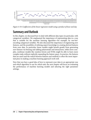
![CHAPTER 5
Model Evaluation and Improvement
Having discussed the fundamentals of supervised and unsupervised learning, and
having explored a variety of machine learning algorithms, we will now dive more
deeply into evaluating models and selecting parameters.
We will focus on the supervised methods, regression and classification, as evaluating
and selecting models in unsupervised learning is often a very qualitative process (as
we saw in Chapter 3).
To evaluate our supervised models, so far we have split our dataset into a training set
and a test set using the train_test_split function, built a model on the training set
by calling the fit method, and evaluated it on the test set using the score method,
which for classification computes the fraction of correctly classified samples. Here’s
an example of that process:
In[2]:
from sklearn.datasets import make_blobs
from sklearn.linear_model import LogisticRegression
from sklearn.model_selection import train_test_split
# create a synthetic dataset
X, y = make_blobs(random_state=0)
# split data and labels into a training and a test set
X_train, X_test, y_train, y_test = train_test_split(X, y, random_state=0)
# instantiate a model and fit it to the training set
logreg = LogisticRegression().fit(X_train, y_train)
# evaluate the model on the test set
print("Test set score: {:.2f}".format(logreg.score(X_test, y_test)))
Out[2]:
Test set score: 0.88
251](https://image.slidesharecdn.com/introductiontomachinelearningwithpythonpdfdrive-230107170822-bfb01dbd/85/Introduction-to-Machine-Learning-with-Python-PDFDrive-com-pdf-265-320.jpg)
![Remember, the reason we split our data into training and test sets is that we are inter‐
ested in measuring how well our model generalizes to new, previously unseen data.
We are not interested in how well our model fit the training set, but rather in how
well it can make predictions for data that was not observed during training.
In this chapter, we will expand on two aspects of this evaluation. We will first intro‐
duce cross-validation, a more robust way to assess generalization performance, and
discuss methods to evaluate classification and regression performance that go beyond
the default measures of accuracy and R2
provided by the score method.
We will also discuss grid search, an effective method for adjusting the parameters in
supervised models for the best generalization performance.
Cross-Validation
Cross-validation is a statistical method of evaluating generalization performance that
is more stable and thorough than using a split into a training and a test set. In cross-
validation, the data is instead split repeatedly and multiple models are trained. The
most commonly used version of cross-validation is k-fold cross-validation, where k is
a user-specified number, usually 5 or 10. When performing five-fold cross-validation,
the data is first partitioned into five parts of (approximately) equal size, called folds.
Next, a sequence of models is trained. The first model is trained using the first fold as
the test set, and the remaining folds (2–5) are used as the training set. The model is
built using the data in folds 2–5, and then the accuracy is evaluated on fold 1. Then
another model is built, this time using fold 2 as the test set and the data in folds 1, 3,
4, and 5 as the training set. This process is repeated using folds 3, 4, and 5 as test sets.
For each of these five splits of the data into training and test sets, we compute the
accuracy. In the end, we have collected five accuracy values. The process is illustrated
in Figure 5-1:
In[3]:
mglearn.plots.plot_cross_validation()
Figure 5-1. Data splitting in five-fold cross-validation
Usually, the first fifth of the data is the first fold, the second fifth of the data is the
second fold, and so on.
252 | Chapter 5: Model Evaluation and Improvement](https://image.slidesharecdn.com/introductiontomachinelearningwithpythonpdfdrive-230107170822-bfb01dbd/85/Introduction-to-Machine-Learning-with-Python-PDFDrive-com-pdf-266-320.jpg)
![Cross-Validation in scikit-learn
Cross-validation is implemented in scikit-learn using the cross_val_score func‐
tion from the model_selection module. The parameters of the cross_val_score
function are the model we want to evaluate, the training data, and the ground-truth
labels. Let’s evaluate LogisticRegression on the iris dataset:
In[4]:
from sklearn.model_selection import cross_val_score
from sklearn.datasets import load_iris
from sklearn.linear_model import LogisticRegression
iris = load_iris()
logreg = LogisticRegression()
scores = cross_val_score(logreg, iris.data, iris.target)
print("Cross-validation scores: {}".format(scores))
Out[4]:
Cross-validation scores: [ 0.961 0.922 0.958]
By default, cross_val_score performs three-fold cross-validation, returning three
accuracy values. We can change the number of folds used by changing the cv parame‐
ter:
In[5]:
scores = cross_val_score(logreg, iris.data, iris.target, cv=5)
print("Cross-validation scores: {}".format(scores))
Out[5]:
Cross-validation scores: [ 1. 0.967 0.933 0.9 1. ]
A common way to summarize the cross-validation accuracy is to compute the mean:
In[6]:
print("Average cross-validation score: {:.2f}".format(scores.mean()))
Out[6]:
Average cross-validation score: 0.96
Using the mean cross-validation we can conclude that we expect the model to be
around 96% accurate on average. Looking at all five scores produced by the five-fold
cross-validation, we can also conclude that there is a relatively high variance in the
accuracy between folds, ranging from 100% accuracy to 90% accuracy. This could
imply that the model is very dependent on the particular folds used for training, but it
could also just be a consequence of the small size of the dataset.
Cross-Validation | 253](https://image.slidesharecdn.com/introductiontomachinelearningwithpythonpdfdrive-230107170822-bfb01dbd/85/Introduction-to-Machine-Learning-with-Python-PDFDrive-com-pdf-267-320.jpg)
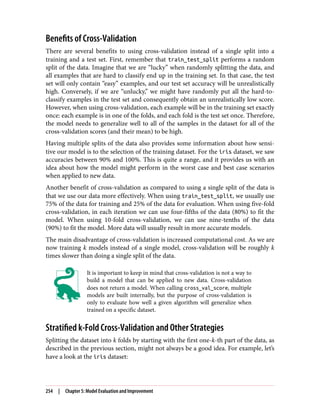
![In[7]:
from sklearn.datasets import load_iris
iris = load_iris()
print("Iris labels:n{}".format(iris.target))
Out[7]:
Iris labels:
[0 0 0 0 0 0 0 0 0 0 0 0 0 0 0 0 0 0 0 0 0 0 0 0 0 0 0 0 0 0 0 0 0 0 0 0 0
0 0 0 0 0 0 0 0 0 0 0 0 0 1 1 1 1 1 1 1 1 1 1 1 1 1 1 1 1 1 1 1 1 1 1 1 1
1 1 1 1 1 1 1 1 1 1 1 1 1 1 1 1 1 1 1 1 1 1 1 1 1 1 2 2 2 2 2 2 2 2 2 2 2
2 2 2 2 2 2 2 2 2 2 2 2 2 2 2 2 2 2 2 2 2 2 2 2 2 2 2 2 2 2 2 2 2 2 2 2 2
2 2]
As you can see, the first third of the data is the class 0, the second third is the class 1,
and the last third is the class 2. Imagine doing three-fold cross-validation on this
dataset. The first fold would be only class 0, so in the first split of the data, the test set
would be only class 0, and the training set would be only classes 1 and 2. As the
classes in training and test sets would be different for all three splits, the three-fold
cross-validation accuracy would be zero on this dataset. That is not very helpful, as
we can do much better than 0% accuracy on iris.
As the simple k-fold strategy fails here, scikit-learn does not use it for classifica‐
tion, but rather uses stratified k-fold cross-validation. In stratified cross-validation, we
split the data such that the proportions between classes are the same in each fold as
they are in the whole dataset, as illustrated in Figure 5-2:
In[8]:
mglearn.plots.plot_stratified_cross_validation()
Figure 5-2. Comparison of standard cross-validation and stratified cross-validation
when the data is ordered by class label
Cross-Validation | 255](https://image.slidesharecdn.com/introductiontomachinelearningwithpythonpdfdrive-230107170822-bfb01dbd/85/Introduction-to-Machine-Learning-with-Python-PDFDrive-com-pdf-269-320.jpg)
![For example, if 90% of your samples belong to class A and 10% of your samples
belong to class B, then stratified cross-validation ensures that in each fold, 90% of
samples belong to class A and 10% of samples belong to class B.
It is usually a good idea to use stratified k-fold cross-validation instead of k-fold
cross-validation to evaluate a classifier, because it results in more reliable estimates of
generalization performance. In the case of only 10% of samples belonging to class B,
using standard k-fold cross-validation it might easily happen that one fold only con‐
tains samples of class A. Using this fold as a test set would not be very informative
about the overall performance of the classifier.
For regression, scikit-learn uses the standard k-fold cross-validation by default. It
would be possible to also try to make each fold representative of the different values
the regression target has, but this is not a commonly used strategy and would be sur‐
prising to most users.
More control over cross-validation
We saw earlier that we can adjust the number of folds that are used in
cross_val_score using the cv parameter. However, scikit-learn allows for much
finer control over what happens during the splitting of the data by providing a cross-
validation splitter as the cv parameter. For most use cases, the defaults of k-fold cross-
validation for regression and stratified k-fold for classification work well, but there
are some cases where you might want to use a different strategy. Say, for example, we
want to use the standard k-fold cross-validation on a classification dataset to repro‐
duce someone else’s results. To do this, we first have to import the KFold splitter class
from the model_selection module and instantiate it with the number of folds we
want to use:
In[9]:
from sklearn.model_selection import KFold
kfold = KFold(n_splits=5)
Then, we can pass the kfold splitter object as the cv parameter to cross_val_score:
In[10]:
print("Cross-validation scores:n{}".format(
cross_val_score(logreg, iris.data, iris.target, cv=kfold)))
Out[10]:
Cross-validation scores:
[ 1. 0.933 0.433 0.967 0.433]
This way, we can verify that it is indeed a really bad idea to use three-fold (nonstrati‐
fied) cross-validation on the iris dataset:
256 | Chapter 5: Model Evaluation and Improvement](https://image.slidesharecdn.com/introductiontomachinelearningwithpythonpdfdrive-230107170822-bfb01dbd/85/Introduction-to-Machine-Learning-with-Python-PDFDrive-com-pdf-270-320.jpg)
![In[11]:
kfold = KFold(n_splits=3)
print("Cross-validation scores:n{}".format(
cross_val_score(logreg, iris.data, iris.target, cv=kfold)))
Out[11]:
Cross-validation scores:
[ 0. 0. 0.]
Remember: each fold corresponds to one of the classes in the iris dataset, and so
nothing can be learned. Another way to resolve this problem is to shuffle the data
instead of stratifying the folds, to remove the ordering of the samples by label. We can
do that by setting the shuffle parameter of KFold to True. If we shuffle the data, we
also need to fix the random_state to get a reproducible shuffling. Otherwise, each run
of cross_val_score would yield a different result, as each time a different split would
be used (this might not be a problem, but can be surprising). Shuffling the data before
splitting it yields a much better result:
In[12]:
kfold = KFold(n_splits=3, shuffle=True, random_state=0)
print("Cross-validation scores:n{}".format(
cross_val_score(logreg, iris.data, iris.target, cv=kfold)))
Out[12]:
Cross-validation scores:
[ 0.9 0.96 0.96]
Leave-one-out cross-validation
Another frequently used cross-validation method is leave-one-out. You can think of
leave-one-out cross-validation as k-fold cross-validation where each fold is a single
sample. For each split, you pick a single data point to be the test set. This can be very
time consuming, particularly for large datasets, but sometimes provides better esti‐
mates on small datasets:
In[13]:
from sklearn.model_selection import LeaveOneOut
loo = LeaveOneOut()
scores = cross_val_score(logreg, iris.data, iris.target, cv=loo)
print("Number of cv iterations: ", len(scores))
print("Mean accuracy: {:.2f}".format(scores.mean()))
Out[13]:
Number of cv iterations: 150
Mean accuracy: 0.95
Cross-Validation | 257](https://image.slidesharecdn.com/introductiontomachinelearningwithpythonpdfdrive-230107170822-bfb01dbd/85/Introduction-to-Machine-Learning-with-Python-PDFDrive-com-pdf-271-320.jpg)
![Shuffle-split cross-validation
Another, very flexible strategy for cross-validation is shuffle-split cross-validation. In
shuffle-split cross-validation, each split samples train_size many points for the
training set and test_size many (disjoint) point for the test set. This splitting is
repeated n_iter times. Figure 5-3 illustrates running four iterations of splitting a
dataset consisting of 10 points, with a training set of 5 points and test sets of 2 points
each (you can use integers for train_size and test_size to use absolute sizes for
these sets, or floating-point numbers to use fractions of the whole dataset):
In[14]:
mglearn.plots.plot_shuffle_split()
Figure 5-3. ShuffleSplit with 10 points, train_size=5, test_size=2, and n_iter=4
The following code splits the dataset into 50% training set and 50% test set for 10
iterations:
In[15]:
from sklearn.model_selection import ShuffleSplit
shuffle_split = ShuffleSplit(test_size=.5, train_size=.5, n_splits=10)
scores = cross_val_score(logreg, iris.data, iris.target, cv=shuffle_split)
print("Cross-validation scores:n{}".format(scores))
Out[15]:
Cross-validation scores:
[ 0.96 0.907 0.947 0.96 0.96 0.907 0.893 0.907 0.92 0.973]
Shuffle-split cross-validation allows for control over the number of iterations inde‐
pendently of the training and test sizes, which can sometimes be helpful. It also allows
for using only part of the data in each iteration, by providing train_size and
test_size settings that don’t add up to one. Subsampling the data in this way can be
useful for experimenting with large datasets.
There is also a stratified variant of ShuffleSplit, aptly named StratifiedShuffleS
plit, which can provide more reliable results for classification tasks.
258 | Chapter 5: Model Evaluation and Improvement](https://image.slidesharecdn.com/introductiontomachinelearningwithpythonpdfdrive-230107170822-bfb01dbd/85/Introduction-to-Machine-Learning-with-Python-PDFDrive-com-pdf-272-320.jpg)
![Cross-validation with groups
Another very common setting for cross-validation is when there are groups in the
data that are highly related. Say you want to build a system to recognize emotions
from pictures of faces, and you collect a dataset of pictures of 100 people where each
person is captured multiple times, showing various emotions. The goal is to build a
classifier that can correctly identify emotions of people not in the dataset. You could
use the default stratified cross-validation to measure the performance of a classifier
here. However, it is likely that pictures of the same person will be in both the training
and the test set. It will be much easier for a classifier to detect emotions in a face that
is part of the training set, compared to a completely new face. To accurately evaluate
the generalization to new faces, we must therefore ensure that the training and test
sets contain images of different people.
To achieve this, we can use GroupKFold, which takes an array of groups as argument
that we can use to indicate which person is in the image. The groups array here indi‐
cates groups in the data that should not be split when creating the training and test
sets, and should not be confused with the class label.
This example of groups in the data is common in medical applications, where you
might have multiple samples from the same patient, but are interested in generalizing
to new patients. Similarly, in speech recognition, you might have multiple recordings
of the same speaker in your dataset, but are interested in recognizing speech of new
speakers.
The following is an example of using a synthetic dataset with a grouping given by the
groups array. The dataset consists of 12 data points, and for each of the data points,
groups specifies which group (think patient) the point belongs to. The groups specify
that there are four groups, and the first three samples belong to the first group, the
next four samples belong to the second group, and so on:
In[17]:
from sklearn.model_selection import GroupKFold
# create synthetic dataset
X, y = make_blobs(n_samples=12, random_state=0)
# assume the first three samples belong to the same group,
# then the next four, etc.
groups = [0, 0, 0, 1, 1, 1, 1, 2, 2, 3, 3, 3]
scores = cross_val_score(logreg, X, y, groups, cv=GroupKFold(n_splits=3))
print("Cross-validation scores:n{}".format(scores))
Out[17]:
Cross-validation scores:
[ 0.75 0.8 0.667]
The samples don’t need to be ordered by group; we just did this for illustration pur‐
poses. The splits that are calculated based on these labels are visualized in Figure 5-4.
Cross-Validation | 259](https://image.slidesharecdn.com/introductiontomachinelearningwithpythonpdfdrive-230107170822-bfb01dbd/85/Introduction-to-Machine-Learning-with-Python-PDFDrive-com-pdf-273-320.jpg)
![As you can see, for each split, each group is either entirely in the training set or
entirely in the test set:
In[16]:
mglearn.plots.plot_label_kfold()
Figure 5-4. Label-dependent splitting with GroupKFold
There are more splitting strategies for cross-validation in scikit-learn, which allow
for an even greater variety of use cases (you can find these in the scikit-learn user
guide). However, the standard KFold, StratifiedKFold, and GroupKFold are by far
the most commonly used ones.
Grid Search
Now that we know how to evaluate how well a model generalizes, we can take the
next step and improve the model’s generalization performance by tuning its parame‐
ters. We discussed the parameter settings of many of the algorithms in scikit-learn
in Chapters 2 and 3, and it is important to understand what the parameters mean
before trying to adjust them. Finding the values of the important parameters of a
model (the ones that provide the best generalization performance) is a tricky task, but
necessary for almost all models and datasets. Because it is such a common task, there
are standard methods in scikit-learn to help you with it. The most commonly used
method is grid search, which basically means trying all possible combinations of the
parameters of interest.
Consider the case of a kernel SVM with an RBF (radial basis function) kernel, as
implemented in the SVC class. As we discussed in Chapter 2, there are two important
parameters: the kernel bandwidth, gamma, and the regularization parameter, C. Say we
want to try the values 0.001, 0.01, 0.1, 1, 10, and 100 for the parameter C, and the
same for gamma. Because we have six different settings for C and gamma that we want to
try, we have 36 combinations of parameters in total. Looking at all possible combina‐
tions creates a table (or grid) of parameter settings for the SVM, as shown here:
260 | Chapter 5: Model Evaluation and Improvement](https://image.slidesharecdn.com/introductiontomachinelearningwithpythonpdfdrive-230107170822-bfb01dbd/85/Introduction-to-Machine-Learning-with-Python-PDFDrive-com-pdf-274-320.jpg)
![C = 0.001 C = 0.01 … C = 10
gamma=0.001 SVC(C=0.001, gamma=0.001) SVC(C=0.01, gamma=0.001) … SVC(C=10, gamma=0.001)
gamma=0.01 SVC(C=0.001, gamma=0.01) SVC(C=0.01, gamma=0.01) … SVC(C=10, gamma=0.01)
… … … … …
gamma=100 SVC(C=0.001, gamma=100) SVC(C=0.01, gamma=100) … SVC(C=10, gamma=100)
Simple Grid Search
We can implement a simple grid search just as for loops over the two parameters,
training and evaluating a classifier for each combination:
In[18]:
# naive grid search implementation
from sklearn.svm import SVC
X_train, X_test, y_train, y_test = train_test_split(
iris.data, iris.target, random_state=0)
print("Size of training set: {} size of test set: {}".format(
X_train.shape[0], X_test.shape[0]))
best_score = 0
for gamma in [0.001, 0.01, 0.1, 1, 10, 100]:
for C in [0.001, 0.01, 0.1, 1, 10, 100]:
# for each combination of parameters, train an SVC
svm = SVC(gamma=gamma, C=C)
svm.fit(X_train, y_train)
# evaluate the SVC on the test set
score = svm.score(X_test, y_test)
# if we got a better score, store the score and parameters
if score > best_score:
best_score = score
best_parameters = {'C': C, 'gamma': gamma}
print("Best score: {:.2f}".format(best_score))
print("Best parameters: {}".format(best_parameters))
Out[18]:
Size of training set: 112 size of test set: 38
Best score: 0.97
Best parameters: {'C': 100, 'gamma': 0.001}
The Danger of Overfitting the Parameters and the Validation Set
Given this result, we might be tempted to report that we found a model that performs
with 97% accuracy on our dataset. However, this claim could be overly optimistic (or
just wrong), for the following reason: we tried many different parameters and
Grid Search | 261](https://image.slidesharecdn.com/introductiontomachinelearningwithpythonpdfdrive-230107170822-bfb01dbd/85/Introduction-to-Machine-Learning-with-Python-PDFDrive-com-pdf-275-320.jpg)
![selected the one with best accuracy on the test set, but this accuracy won’t necessarily
carry over to new data. Because we used the test data to adjust the parameters, we can
no longer use it to assess how good the model is. This is the same reason we needed
to split the data into training and test sets in the first place; we need an independent
dataset to evaluate, one that was not used to create the model.
One way to resolve this problem is to split the data again, so we have three sets: the
training set to build the model, the validation (or development) set to select the
parameters of the model, and the test set to evaluate the performance of the selected
parameters. Figure 5-5 shows what this looks like:
In[19]:
mglearn.plots.plot_threefold_split()
Figure 5-5. A threefold split of data into training set, validation set, and test set
After selecting the best parameters using the validation set, we can rebuild a model
using the parameter settings we found, but now training on both the training data
and the validation data. This way, we can use as much data as possible to build our
model. This leads to the following implementation:
In[20]:
from sklearn.svm import SVC
# split data into train+validation set and test set
X_trainval, X_test, y_trainval, y_test = train_test_split(
iris.data, iris.target, random_state=0)
# split train+validation set into training and validation sets
X_train, X_valid, y_train, y_valid = train_test_split(
X_trainval, y_trainval, random_state=1)
print("Size of training set: {} size of validation set: {} size of test set:"
" {}n".format(X_train.shape[0], X_valid.shape[0], X_test.shape[0]))
best_score = 0
for gamma in [0.001, 0.01, 0.1, 1, 10, 100]:
for C in [0.001, 0.01, 0.1, 1, 10, 100]:
# for each combination of parameters, train an SVC
svm = SVC(gamma=gamma, C=C)
svm.fit(X_train, y_train)
# evaluate the SVC on the test set
score = svm.score(X_valid, y_valid)
# if we got a better score, store the score and parameters
if score > best_score:
best_score = score
best_parameters = {'C': C, 'gamma': gamma}
262 | Chapter 5: Model Evaluation and Improvement](https://image.slidesharecdn.com/introductiontomachinelearningwithpythonpdfdrive-230107170822-bfb01dbd/85/Introduction-to-Machine-Learning-with-Python-PDFDrive-com-pdf-276-320.jpg)
![# rebuild a model on the combined training and validation set,
# and evaluate it on the test set
svm = SVC(**best_parameters)
svm.fit(X_trainval, y_trainval)
test_score = svm.score(X_test, y_test)
print("Best score on validation set: {:.2f}".format(best_score))
print("Best parameters: ", best_parameters)
print("Test set score with best parameters: {:.2f}".format(test_score))
Out[20]:
Size of training set: 84 size of validation set: 28 size of test set: 38
Best score on validation set: 0.96
Best parameters: {'C': 10, 'gamma': 0.001}
Test set score with best parameters: 0.92
The best score on the validation set is 96%: slightly lower than before, probably
because we used less data to train the model (X_train is smaller now because we split
our dataset twice). However, the score on the test set—the score that actually tells us
how well we generalize—is even lower, at 92%. So we can only claim to classify new
data 92% correctly, not 97% correctly as we thought before!
The distinction between the training set, validation set, and test set is fundamentally
important to applying machine learning methods in practice. Any choices made
based on the test set accuracy “leak” information from the test set into the model.
Therefore, it is important to keep a separate test set, which is only used for the final
evaluation. It is good practice to do all exploratory analysis and model selection using
the combination of a training and a validation set, and reserve the test set for a final
evaluation—this is even true for exploratory visualization. Strictly speaking, evaluat‐
ing more than one model on the test set and choosing the better of the two will result
in an overly optimistic estimate of how accurate the model is.
Grid Search with Cross-Validation
While the method of splitting the data into a training, a validation, and a test set that
we just saw is workable, and relatively commonly used, it is quite sensitive to how
exactly the data is split. From the output of the previous code snippet we can see that
GridSearchCV selects 'C': 10, 'gamma': 0.001 as the best parameters, while the
output of the code in the previous section selects 'C': 100, 'gamma': 0.001 as the
best parameters. For a better estimate of the generalization performance, instead of
using a single split into a training and a validation set, we can use cross-validation to
evaluate the performance of each parameter combination. This method can be coded
up as follows:
Grid Search | 263](https://image.slidesharecdn.com/introductiontomachinelearningwithpythonpdfdrive-230107170822-bfb01dbd/85/Introduction-to-Machine-Learning-with-Python-PDFDrive-com-pdf-277-320.jpg)
![In[21]:
for gamma in [0.001, 0.01, 0.1, 1, 10, 100]:
for C in [0.001, 0.01, 0.1, 1, 10, 100]:
# for each combination of parameters,
# train an SVC
svm = SVC(gamma=gamma, C=C)
# perform cross-validation
scores = cross_val_score(svm, X_trainval, y_trainval, cv=5)
# compute mean cross-validation accuracy
score = np.mean(scores)
# if we got a better score, store the score and parameters
if score > best_score:
best_score = score
best_parameters = {'C': C, 'gamma': gamma}
# rebuild a model on the combined training and validation set
svm = SVC(**best_parameters)
svm.fit(X_trainval, y_trainval)
To evaluate the accuracy of the SVM using a particular setting of C and gamma using
five-fold cross-validation, we need to train 36 * 5 = 180 models. As you can imagine,
the main downside of the use of cross-validation is the time it takes to train all these
models.
The following visualization (Figure 5-6) illustrates how the best parameter setting is
selected in the preceding code:
In[22]:
mglearn.plots.plot_cross_val_selection()
Figure 5-6. Results of grid search with cross-validation
For each parameter setting (only a subset is shown), five accuracy values are compu‐
ted, one for each split in the cross-validation. Then the mean validation accuracy is
computed for each parameter setting. The parameters with the highest mean valida‐
tion accuracy are chosen, marked by the circle.
264 | Chapter 5: Model Evaluation and Improvement](https://image.slidesharecdn.com/introductiontomachinelearningwithpythonpdfdrive-230107170822-bfb01dbd/85/Introduction-to-Machine-Learning-with-Python-PDFDrive-com-pdf-278-320.jpg)
![As we said earlier, cross-validation is a way to evaluate a given algo‐
rithm on a specific dataset. However, it is often used in conjunction
with parameter search methods like grid search. For this reason,
many people use the term cross-validation colloquially to refer to
grid search with cross-validation.
The overall process of splitting the data, running the grid search, and evaluating the
final parameters is illustrated in Figure 5-7:
In[23]:
mglearn.plots.plot_grid_search_overview()
Figure 5-7. Overview of the process of parameter selection and model evaluation with
GridSearchCV
Because grid search with cross-validation is such a commonly used method to adjust
parameters, scikit-learn provides the GridSearchCV class, which implements it in
the form of an estimator. To use the GridSearchCV class, you first need to specify the
parameters you want to search over using a dictionary. GridSearchCV will then per‐
form all the necessary model fits. The keys of the dictionary are the names of parame‐
ters we want to adjust (as given when constructing the model—in this case, C and
gamma), and the values are the parameter settings we want to try out. Trying the val‐
ues 0.001, 0.01, 0.1, 1, 10, and 100 for C and gamma translates to the following
dictionary:
In[24]:
param_grid = {'C': [0.001, 0.01, 0.1, 1, 10, 100],
'gamma': [0.001, 0.01, 0.1, 1, 10, 100]}
print("Parameter grid:n{}".format(param_grid))
Out[24]:
Parameter grid:
{'C': [0.001, 0.01, 0.1, 1, 10, 100], 'gamma': [0.001, 0.01, 0.1, 1, 10, 100]}
Grid Search | 265](https://image.slidesharecdn.com/introductiontomachinelearningwithpythonpdfdrive-230107170822-bfb01dbd/85/Introduction-to-Machine-Learning-with-Python-PDFDrive-com-pdf-279-320.jpg)
![1 A scikit-learn estimator that is created using another estimator is called a meta-estimator. GridSearchCV is
the most commonly used meta-estimator, but we will see more later.
We can now instantiate the GridSearchCV class with the model (SVC), the parameter
grid to search (param_grid), and the cross-validation strategy we want to use (say,
five-fold stratified cross-validation):
In[25]:
from sklearn.model_selection import GridSearchCV
from sklearn.svm import SVC
grid_search = GridSearchCV(SVC(), param_grid, cv=5)
GridSearchCV will use cross-validation in place of the split into a training and valida‐
tion set that we used before. However, we still need to split the data into a training
and a test set, to avoid overfitting the parameters:
In[26]:
X_train, X_test, y_train, y_test = train_test_split(
iris.data, iris.target, random_state=0)
The grid_search object that we created behaves just like a classifier; we can call the
standard methods fit, predict, and score on it.1
However, when we call fit, it will
run cross-validation for each combination of parameters we specified in param_grid:
In[27]:
grid_search.fit(X_train, y_train)
Fitting the GridSearchCV object not only searches for the best parameters, but also
automatically fits a new model on the whole training dataset with the parameters that
yielded the best cross-validation performance. What happens in fit is therefore
equivalent to the result of the In[21] code we saw at the beginning of this section. The
GridSearchCV class provides a very convenient interface to access the retrained
model using the predict and score methods. To evaluate how well the best found
parameters generalize, we can call score on the test set:
In[28]:
print("Test set score: {:.2f}".format(grid_search.score(X_test, y_test)))
Out[28]:
Test set score: 0.97
Choosing the parameters using cross-validation, we actually found a model that ach‐
ieves 97% accuracy on the test set. The important thing here is that we did not use the
test set to choose the parameters. The parameters that were found are scored in the
266 | Chapter 5: Model Evaluation and Improvement](https://image.slidesharecdn.com/introductiontomachinelearningwithpythonpdfdrive-230107170822-bfb01dbd/85/Introduction-to-Machine-Learning-with-Python-PDFDrive-com-pdf-280-320.jpg)
![best_params_ attribute, and the best cross-validation accuracy (the mean accuracy
over the different splits for this parameter setting) is stored in best_score_:
In[29]:
print("Best parameters: {}".format(grid_search.best_params_))
print("Best cross-validation score: {:.2f}".format(grid_search.best_score_))
Out[29]:
Best parameters: {'C': 100, 'gamma': 0.01}
Best cross-validation score: 0.97
Again, be careful not to confuse best_score_ with the generaliza‐
tion performance of the model as computed by the score method
on the test set. Using the score method (or evaluating the output of
the predict method) employs a model trained on the whole train‐
ing set. The best_score_ attribute stores the mean cross-validation
accuracy, with cross-validation performed on the training set.
Sometimes it is helpful to have access to the actual model that was found—for exam‐
ple, to look at coefficients or feature importances. You can access the model with the
best parameters trained on the whole training set using the best_estimator_
attribute:
In[30]:
print("Best estimator:n{}".format(grid_search.best_estimator_))
Out[30]:
Best estimator:
SVC(C=100, cache_size=200, class_weight=None, coef0=0.0,
decision_function_shape=None, degree=3, gamma=0.01, kernel='rbf',
max_iter=-1, probability=False, random_state=None, shrinking=True,
tol=0.001, verbose=False)
Because grid_search itself has predict and score methods, using best_estimator_
is not needed to make predictions or evaluate the model.
Analyzing the result of cross-validation
It is often helpful to visualize the results of cross-validation, to understand how the
model generalization depends on the parameters we are searching. As grid searches
are quite computationally expensive to run, often it is a good idea to start with a rela‐
tively coarse and small grid. We can then inspect the results of the cross-validated
grid search, and possibly expand our search. The results of a grid search can be found
in the cv_results_ attribute, which is a dictionary storing all aspects of the search. It
Grid Search | 267](https://image.slidesharecdn.com/introductiontomachinelearningwithpythonpdfdrive-230107170822-bfb01dbd/85/Introduction-to-Machine-Learning-with-Python-PDFDrive-com-pdf-281-320.jpg)
![contains a lot of details, as you can see in the following output, and is best looked at
after converting it to a pandas DataFrame:
In[31]:
import pandas as pd
# convert to DataFrame
results = pd.DataFrame(grid_search.cv_results_)
# show the first 5 rows
display(results.head())
Out[31]:
param_C param_gamma params mean_test_score
0 0.001 0.001 {'C': 0.001, 'gamma': 0.001} 0.366
1 0.001 0.01 {'C': 0.001, 'gamma': 0.01} 0.366
2 0.001 0.1 {'C': 0.001, 'gamma': 0.1} 0.366
3 0.001 1 {'C': 0.001, 'gamma': 1} 0.366
4 0.001 10 {'C': 0.001, 'gamma': 10} 0.366
rank_test_score split0_test_score split1_test_score split2_test_score
0 22 0.375 0.347 0.363
1 22 0.375 0.347 0.363
2 22 0.375 0.347 0.363
3 22 0.375 0.347 0.363
4 22 0.375 0.347 0.363
split3_test_score split4_test_score std_test_score
0 0.363 0.380 0.011
1 0.363 0.380 0.011
2 0.363 0.380 0.011
3 0.363 0.380 0.011
4 0.363 0.380 0.011
Each row in results corresponds to one particular parameter setting. For each set‐
ting, the results of all cross-validation splits are recorded, as well as the mean and
standard deviation over all splits. As we were searching a two-dimensional grid of
parameters (C and gamma), this is best visualized as a heat map (Figure 5-8). First we
extract the mean validation scores, then we reshape the scores so that the axes corre‐
spond to C and gamma:
In[32]:
scores = np.array(results.mean_test_score).reshape(6, 6)
# plot the mean cross-validation scores
mglearn.tools.heatmap(scores, xlabel='gamma', xticklabels=param_grid['gamma'],
ylabel='C', yticklabels=param_grid['C'], cmap="viridis")
268 | Chapter 5: Model Evaluation and Improvement](https://image.slidesharecdn.com/introductiontomachinelearningwithpythonpdfdrive-230107170822-bfb01dbd/85/Introduction-to-Machine-Learning-with-Python-PDFDrive-com-pdf-282-320.jpg)
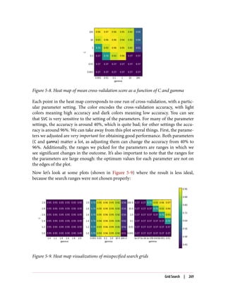
![In[33]:
fig, axes = plt.subplots(1, 3, figsize=(13, 5))
param_grid_linear = {'C': np.linspace(1, 2, 6),
'gamma': np.linspace(1, 2, 6)}
param_grid_one_log = {'C': np.linspace(1, 2, 6),
'gamma': np.logspace(-3, 2, 6)}
param_grid_range = {'C': np.logspace(-3, 2, 6),
'gamma': np.logspace(-7, -2, 6)}
for param_grid, ax in zip([param_grid_linear, param_grid_one_log,
param_grid_range], axes):
grid_search = GridSearchCV(SVC(), param_grid, cv=5)
grid_search.fit(X_train, y_train)
scores = grid_search.cv_results_['mean_test_score'].reshape(6, 6)
# plot the mean cross-validation scores
scores_image = mglearn.tools.heatmap(
scores, xlabel='gamma', ylabel='C', xticklabels=param_grid['gamma'],
yticklabels=param_grid['C'], cmap="viridis", ax=ax)
plt.colorbar(scores_image, ax=axes.tolist())
The first panel shows no changes at all, with a constant color over the whole parame‐
ter grid. In this case, this is caused by improper scaling and range of the parameters C
and gamma. However, if no change in accuracy is visible over the different parameter
settings, it could also be that a parameter is just not important at all. It is usually good
to try very extreme values first, to see if there are any changes in the accuracy as a
result of changing a parameter.
The second panel shows a vertical stripe pattern. This indicates that only the setting
of the gamma parameter makes any difference. This could mean that the gamma param‐
eter is searching over interesting values but the C parameter is not—or it could mean
the C parameter is not important.
The third panel shows changes in both C and gamma. However, we can see that in the
entire bottom left of the plot, nothing interesting is happening. We can probably
exclude the very small values from future grid searches. The optimum parameter set‐
ting is at the top right. As the optimum is in the border of the plot, we can expect that
there might be even better values beyond this border, and we might want to change
our search range to include more parameters in this region.
Tuning the parameter grid based on the cross-validation scores is perfectly fine, and a
good way to explore the importance of different parameters. However, you should
not test different parameter ranges on the final test set—as we discussed earlier, eval‐
270 | Chapter 5: Model Evaluation and Improvement](https://image.slidesharecdn.com/introductiontomachinelearningwithpythonpdfdrive-230107170822-bfb01dbd/85/Introduction-to-Machine-Learning-with-Python-PDFDrive-com-pdf-284-320.jpg)
![uation of the test set should happen only once we know exactly what model we want
to use.
Search over spaces that are not grids
In some cases, trying all possible combinations of all parameters as GridSearchCV
usually does, is not a good idea. For example, SVC has a kernel parameter, and
depending on which kernel is chosen, other parameters will be relevant. If ker
nel='linear', the model is linear, and only the C parameter is used. If kernel='rbf',
both the C and gamma parameters are used (but not other parameters like degree). In
this case, searching over all possible combinations of C, gamma, and kernel wouldn’t
make sense: if kernel='linear', gamma is not used, and trying different values for
gamma would be a waste of time. To deal with these kinds of “conditional” parameters,
GridSearchCV allows the param_grid to be a list of dictionaries. Each dictionary in the
list is expanded into an independent grid. A possible grid search involving kernel and
parameters could look like this:
In[34]:
param_grid = [{'kernel': ['rbf'],
'C': [0.001, 0.01, 0.1, 1, 10, 100],
'gamma': [0.001, 0.01, 0.1, 1, 10, 100]},
{'kernel': ['linear'],
'C': [0.001, 0.01, 0.1, 1, 10, 100]}]
print("List of grids:n{}".format(param_grid))
Out[34]:
List of grids:
[{'kernel': ['rbf'], 'C': [0.001, 0.01, 0.1, 1, 10, 100],
'gamma': [0.001, 0.01, 0.1, 1, 10, 100]},
{'kernel': ['linear'], 'C': [0.001, 0.01, 0.1, 1, 10, 100]}]
In the first grid, the kernel parameter is always set to 'rbf' (not that the entry for
kernel is a list of length one), and both the C and gamma parameters are varied. In the
second grid, the kernel parameter is always set to linear, and only C is varied. Now
let’s apply this more complex parameter search:
In[35]:
grid_search = GridSearchCV(SVC(), param_grid, cv=5)
grid_search.fit(X_train, y_train)
print("Best parameters: {}".format(grid_search.best_params_))
print("Best cross-validation score: {:.2f}".format(grid_search.best_score_))
Out[35]:
Best parameters: {'C': 100, 'kernel': 'rbf', 'gamma': 0.01}
Best cross-validation score: 0.97
Grid Search | 271](https://image.slidesharecdn.com/introductiontomachinelearningwithpythonpdfdrive-230107170822-bfb01dbd/85/Introduction-to-Machine-Learning-with-Python-PDFDrive-com-pdf-285-320.jpg)
![Let’s look at the cv_results_ again. As expected, if kernel is 'linear', then only C is
varied:
In[36]:
results = pd.DataFrame(grid_search.cv_results_)
# we display the transposed table so that it better fits on the page:
display(results.T)
Out[36]:
0 1 2 3 … 38 39 40 41
param_C 0.001 0.001 0.001 0.001 … 0.1 1 10 100
param_gamma 0.001 0.01 0.1 1 … NaN NaN NaN NaN
param_kernel rbf rbf rbf rbf … linear linear linear linear
params {C: 0.001,
kernel: rbf,
gamma:
0.001}
{C: 0.001,
kernel: rbf,
gamma:
0.01}
{C: 0.001,
kernel: rbf,
gamma:
0.1}
{C: 0.001,
kernel: rbf,
gamma: 1}
… {C: 0.1,
kernel:
linear}
{C: 1,
kernel:
linear}
{C: 10,
kernel:
linear}
{C: 100,
kernel:
linear}
mean_test_score 0.37 0.37 0.37 0.37 … 0.95 0.97 0.96 0.96
rank_test_score 27 27 27 27 … 11 1 3 3
split0_test_score 0.38 0.38 0.38 0.38 … 0.96 1 0.96 0.96
split1_test_score 0.35 0.35 0.35 0.35 … 0.91 0.96 1 1
split2_test_score 0.36 0.36 0.36 0.36 … 1 1 1 1
split3_test_score 0.36 0.36 0.36 0.36 … 0.91 0.95 0.91 0.91
split4_test_score 0.38 0.38 0.38 0.38 … 0.95 0.95 0.95 0.95
std_test_score 0.011 0.011 0.011 0.011 … 0.033 0.022 0.034 0.034
12 rows × 42 columns
Using different cross-validation strategies with grid search
Similarly to cross_val_score, GridSearchCV uses stratified k-fold cross-validation
by default for classification, and k-fold cross-validation for regression. However, you
can also pass any cross-validation splitter, as described in “More control over cross-
validation” on page 256, as the cv parameter in GridSearchCV. In particular, to get
only a single split into a training and a validation set, you can use ShuffleSplit or
StratifiedShuffleSplit with n_iter=1. This might be helpful for very large data‐
sets, or very slow models.
Nested cross-validation
In the preceding examples, we went from using a single split of the data into training,
validation, and test sets to splitting the data into training and test sets and then per‐
forming cross-validation on the training set. But when using GridSearchCV as
272 | Chapter 5: Model Evaluation and Improvement](https://image.slidesharecdn.com/introductiontomachinelearningwithpythonpdfdrive-230107170822-bfb01dbd/85/Introduction-to-Machine-Learning-with-Python-PDFDrive-com-pdf-286-320.jpg)
![described earlier, we still have a single split of the data into training and test sets,
which might make our results unstable and make us depend too much on this single
split of the data. We can go a step further, and instead of splitting the original data
into training and test sets once, use multiple splits of cross-validation. This will result
in what is called nested cross-validation. In nested cross-validation, there is an outer
loop over splits of the data into training and test sets. For each of them, a grid search
is run (which might result in different best parameters for each split in the outer
loop). Then, for each outer split, the test set score using the best settings is reported.
The result of this procedure is a list of scores—not a model, and not a parameter set‐
ting. The scores tell us how well a model generalizes, given the best parameters found
by the grid. As it doesn’t provide a model that can be used on new data, nested cross-
validation is rarely used when looking for a predictive model to apply to future data.
However, it can be useful for evaluating how well a given model works on a particular
dataset.
Implementing nested cross-validation in scikit-learn is straightforward. We call
cross_val_score with an instance of GridSearchCV as the model:
In[34]:
scores = cross_val_score(GridSearchCV(SVC(), param_grid, cv=5),
iris.data, iris.target, cv=5)
print("Cross-validation scores: ", scores)
print("Mean cross-validation score: ", scores.mean())
Out[34]:
Cross-validation scores: [ 0.967 1. 0.967 0.967 1. ]
Mean cross-validation score: 0.98
The result of our nested cross-validation can be summarized as “SVC can achieve 98%
mean cross-validation accuracy on the iris dataset”—nothing more and nothing
less.
Here, we used stratified five-fold cross-validation in both the inner and the outer
loop. As our param_grid contains 36 combinations of parameters, this results in a
whopping 36 * 5 * 5 = 900 models being built, making nested cross-validation a very
expensive procedure. Here, we used the same cross-validation splitter in the inner
and the outer loop; however, this is not necessary and you can use any combination
of cross-validation strategies in the inner and outer loops. It can be a bit tricky to
understand what is happening in the single line given above, and it can be helpful to
visualize it as for loops, as done in the following simplified implementation:
Grid Search | 273](https://image.slidesharecdn.com/introductiontomachinelearningwithpythonpdfdrive-230107170822-bfb01dbd/85/Introduction-to-Machine-Learning-with-Python-PDFDrive-com-pdf-287-320.jpg)
![In[35]:
def nested_cv(X, y, inner_cv, outer_cv, Classifier, parameter_grid):
outer_scores = []
# for each split of the data in the outer cross-validation
# (split method returns indices)
for training_samples, test_samples in outer_cv.split(X, y):
# find best parameter using inner cross-validation
best_parms = {}
best_score = -np.inf
# iterate over parameters
for parameters in parameter_grid:
# accumulate score over inner splits
cv_scores = []
# iterate over inner cross-validation
for inner_train, inner_test in inner_cv.split(
X[training_samples], y[training_samples]):
# build classifier given parameters and training data
clf = Classifier(**parameters)
clf.fit(X[inner_train], y[inner_train])
# evaluate on inner test set
score = clf.score(X[inner_test], y[inner_test])
cv_scores.append(score)
# compute mean score over inner folds
mean_score = np.mean(cv_scores)
if mean_score > best_score:
# if better than so far, remember parameters
best_score = mean_score
best_params = parameters
# build classifier on best parameters using outer training set
clf = Classifier(**best_params)
clf.fit(X[training_samples], y[training_samples])
# evaluate
outer_scores.append(clf.score(X[test_samples], y[test_samples]))
return np.array(outer_scores)
Now, let’s run this function on the iris dataset:
In[36]:
from sklearn.model_selection import ParameterGrid, StratifiedKFold
scores = nested_cv(iris.data, iris.target, StratifiedKFold(5),
StratifiedKFold(5), SVC, ParameterGrid(param_grid))
print("Cross-validation scores: {}".format(scores))
Out[36]:
Cross-validation scores: [ 0.967 1. 0.967 0.967 1. ]
Parallelizing cross-validation and grid search
While running a grid search over many parameters and on large datasets can be com‐
putationally challenging, it is also embarrassingly parallel. This means that building a
274 | Chapter 5: Model Evaluation and Improvement](https://image.slidesharecdn.com/introductiontomachinelearningwithpythonpdfdrive-230107170822-bfb01dbd/85/Introduction-to-Machine-Learning-with-Python-PDFDrive-com-pdf-288-320.jpg)
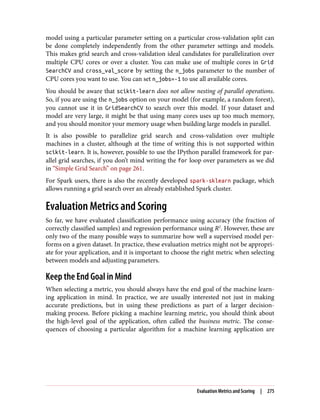
![class imbalance into account. You can achieve 99% accuracy without building a
machine learning model, by always predicting “no click.” On the other hand, even
with imbalanced data, a 99% accurate model could in fact be quite good. However,
accuracy doesn’t allow us to distinguish the constant “no click” model from a poten‐
tially good model.
To illustrate, we’ll create a 9:1 imbalanced dataset from the digits dataset, by classify‐
ing the digit 9 against the nine other classes:
In[37]:
from sklearn.datasets import load_digits
digits = load_digits()
y = digits.target == 9
X_train, X_test, y_train, y_test = train_test_split(
digits.data, y, random_state=0)
We can use the DummyClassifier to always predict the majority class (here
“not nine”) to see how uninformative accuracy can be:
In[38]:
from sklearn.dummy import DummyClassifier
dummy_majority = DummyClassifier(strategy='most_frequent').fit(X_train, y_train)
pred_most_frequent = dummy_majority.predict(X_test)
print("Unique predicted labels: {}".format(np.unique(pred_most_frequent)))
print("Test score: {:.2f}".format(dummy_majority.score(X_test, y_test)))
Out[38]:
Unique predicted labels: [False]
Test score: 0.90
We obtained close to 90% accuracy without learning anything. This might seem strik‐
ing, but think about it for a minute. Imagine someone telling you their model is 90%
accurate. You might think they did a very good job. But depending on the problem,
that might be possible by just predicting one class! Let’s compare this against using an
actual classifier:
In[39]:
from sklearn.tree import DecisionTreeClassifier
tree = DecisionTreeClassifier(max_depth=2).fit(X_train, y_train)
pred_tree = tree.predict(X_test)
print("Test score: {:.2f}".format(tree.score(X_test, y_test)))
Out[39]:
Test score: 0.92
278 | Chapter 5: Model Evaluation and Improvement](https://image.slidesharecdn.com/introductiontomachinelearningwithpythonpdfdrive-230107170822-bfb01dbd/85/Introduction-to-Machine-Learning-with-Python-PDFDrive-com-pdf-292-320.jpg)
![According to accuracy, the DecisionTreeClassifier is only slightly better than the
constant predictor. This could indicate either that something is wrong with how we
used DecisionTreeClassifier, or that accuracy is in fact not a good measure here.
For comparison purposes, let’s evaluate two more classifiers, LogisticRegression
and the default DummyClassifier, which makes random predictions but produces
classes with the same proportions as in the training set:
In[40]:
from sklearn.linear_model import LogisticRegression
dummy = DummyClassifier().fit(X_train, y_train)
pred_dummy = dummy.predict(X_test)
print("dummy score: {:.2f}".format(dummy.score(X_test, y_test)))
logreg = LogisticRegression(C=0.1).fit(X_train, y_train)
pred_logreg = logreg.predict(X_test)
print("logreg score: {:.2f}".format(logreg.score(X_test, y_test)))
Out[40]:
dummy score: 0.80
logreg score: 0.98
The dummy classifier that produces random output is clearly the worst of the lot
(according to accuracy), while LogisticRegression produces very good results.
However, even the random classifier yields over 80% accuracy. This makes it very
hard to judge which of these results is actually helpful. The problem here is that accu‐
racy is an inadequate measure for quantifying predictive performance in this imbal‐
anced setting. For the rest of this chapter, we will explore alternative metrics that
provide better guidance in selecting models. In particular, we would like to have met‐
rics that tell us how much better a model is than making “most frequent” predictions
or random predictions, as they are computed in pred_most_frequent and
pred_dummy. If we use a metric to assess our models, it should definitely be able to
weed out these nonsense predictions.
Confusion matrices
One of the most comprehensive ways to represent the result of evaluating binary clas‐
sification is using confusion matrices. Let’s inspect the predictions of LogisticRegres
sion from the previous section using the confusion_matrix function. We already
stored the predictions on the test set in pred_logreg:
Evaluation Metrics and Scoring | 279](https://image.slidesharecdn.com/introductiontomachinelearningwithpythonpdfdrive-230107170822-bfb01dbd/85/Introduction-to-Machine-Learning-with-Python-PDFDrive-com-pdf-293-320.jpg)
![In[41]:
from sklearn.metrics import confusion_matrix
confusion = confusion_matrix(y_test, pred_logreg)
print("Confusion matrix:n{}".format(confusion))
Out[41]:
Confusion matrix:
[[401 2]
[ 8 39]]
The output of confusion_matrix is a two-by-two array, where the rows correspond
to the true classes and the columns correspond to the predicted classes. Each entry
counts how often a sample that belongs to the class corresponding to the row (here,
“not nine” and “nine”) was classified as the class corresponding to the column. The
following plot (Figure 5-10) illustrates this meaning:
In[42]:
mglearn.plots.plot_confusion_matrix_illustration()
Figure 5-10. Confusion matrix of the “nine vs. rest” classification task
280 | Chapter 5: Model Evaluation and Improvement](https://image.slidesharecdn.com/introductiontomachinelearningwithpythonpdfdrive-230107170822-bfb01dbd/85/Introduction-to-Machine-Learning-with-Python-PDFDrive-com-pdf-294-320.jpg)
![3 The main diagonal of a two-dimensional array or matrix A is A[i, i].
Entries on the main diagonal3
of the confusion matrix correspond to correct classifi‐
cations, while other entries tell us how many samples of one class got mistakenly clas‐
sified as another class.
If we declare “a nine” the positive class, we can relate the entries of the confusion
matrix with the terms false positive and false negative that we introduced earlier. To
complete the picture, we call correctly classified samples belonging to the positive
class true positives and correctly classified samples belonging to the negative class true
negatives. These terms are usually abbreviated FP, FN, TP, and TN and lead to the fol‐
lowing interpretation for the confusion matrix (Figure 5-11):
In[43]:
mglearn.plots.plot_binary_confusion_matrix()
Figure 5-11. Confusion matrix for binary classification
Now let’s use the confusion matrix to compare the models we fitted earlier (the two
dummy models, the decision tree, and the logistic regression):
In[44]:
print("Most frequent class:")
print(confusion_matrix(y_test, pred_most_frequent))
print("nDummy model:")
print(confusion_matrix(y_test, pred_dummy))
print("nDecision tree:")
print(confusion_matrix(y_test, pred_tree))
print("nLogistic Regression")
print(confusion_matrix(y_test, pred_logreg))
Evaluation Metrics and Scoring | 281](https://image.slidesharecdn.com/introductiontomachinelearningwithpythonpdfdrive-230107170822-bfb01dbd/85/Introduction-to-Machine-Learning-with-Python-PDFDrive-com-pdf-295-320.jpg)
![Out[44]:
Most frequent class:
[[403 0]
[ 47 0]]
Dummy model:
[[361 42]
[ 43 4]]
Decision tree:
[[390 13]
[ 24 23]]
Logistic Regression
[[401 2]
[ 8 39]]
Looking at the confusion matrix, it is quite clear that something is wrong with
pred_most_frequent, because it always predicts the same class. pred_dummy, on the
other hand, has a very small number of true positives (4), particularly compared to
the number of false negatives and false positives—there are many more false positives
than true positives! The predictions made by the decision tree make much more
sense than the dummy predictions, even though the accuracy was nearly the same.
Finally, we can see that logistic regression does better than pred_tree in all aspects: it
has more true positives and true negatives while having fewer false positives and false
negatives. From this comparison, it is clear that only the decision tree and the logistic
regression give reasonable results, and that the logistic regression works better than
the tree on all accounts. However, inspecting the full confusion matrix is a bit cum‐
bersome, and while we gained a lot of insight from looking at all aspects of the
matrix, the process was very manual and qualitative. There are several ways to sum‐
marize the information in the confusion matrix, which we will discuss next.
Relation to accuracy. We already saw one way to summarize the result in the confu‐
sion matrix—by computing accuracy, which can be expressed as:
Accuracy =
TP+TN
TP+TN + FP + FN
In other words, accuracy is the number of correct predictions (TP and TN) divided
by the number of all samples (all entries of the confusion matrix summed up).
Precision, recall, and f-score. There are several other ways to summarize the confusion
matrix, with the most common ones being precision and recall. Precision measures
how many of the samples predicted as positive are actually positive:
282 | Chapter 5: Model Evaluation and Improvement](https://image.slidesharecdn.com/introductiontomachinelearningwithpythonpdfdrive-230107170822-bfb01dbd/85/Introduction-to-Machine-Learning-with-Python-PDFDrive-com-pdf-296-320.jpg)
![This particular variant is also known as the f1-score. As it takes precision and recall
into account, it can be a better measure than accuracy on imbalanced binary classifi‐
cation datasets. Let’s run it on the predictions for the “nine vs. rest” dataset that we
computed earlier. Here, we will assume that the “nine” class is the positive class (it is
labeled as True while the rest is labeled as False), so the positive class is the minority
class:
In[45]:
from sklearn.metrics import f1_score
print("f1 score most frequent: {:.2f}".format(
f1_score(y_test, pred_most_frequent)))
print("f1 score dummy: {:.2f}".format(f1_score(y_test, pred_dummy)))
print("f1 score tree: {:.2f}".format(f1_score(y_test, pred_tree)))
print("f1 score logistic regression: {:.2f}".format(
f1_score(y_test, pred_logreg)))
Out[45]:
f1 score most frequent: 0.00
f1 score dummy: 0.10
f1 score tree: 0.55
f1 score logistic regression: 0.89
We can note two things here. First, we get an error message for the most_frequent
prediction, as there were no predictions of the positive class (which makes the
denominator in the f-score zero). Also, we can see a pretty strong distinction between
the dummy predictions and the tree predictions, which wasn’t clear when looking at
accuracy alone. Using the f-score for evaluation, we summarized the predictive per‐
formance again in one number. However, the f-score seems to capture our intuition
of what makes a good model much better than accuracy did. A disadvantage of the
f-score, however, is that it is harder to interpret and explain than accuracy.
If we want a more comprehensive summary of precision, recall, and f1-score, we can
use the classification_report convenience function to compute all three at once,
and print them in a nice format:
In[46]:
from sklearn.metrics import classification_report
print(classification_report(y_test, pred_most_frequent,
target_names=["not nine", "nine"]))
284 | Chapter 5: Model Evaluation and Improvement](https://image.slidesharecdn.com/introductiontomachinelearningwithpythonpdfdrive-230107170822-bfb01dbd/85/Introduction-to-Machine-Learning-with-Python-PDFDrive-com-pdf-298-320.jpg)
![Out[46]:
precision recall f1-score support
not nine 0.90 1.00 0.94 403
nine 0.00 0.00 0.00 47
avg / total 0.80 0.90 0.85 450
The classification_report function produces one line per class (here, True and
False) and reports precision, recall, and f-score with this class as the positive class.
Before, we assumed the minority “nine” class was the positive class. If we change the
positive class to “not nine,” we can see from the output of classification_report
that we obtain an f-score of 0.94 with the most_frequent model. Furthermore, for the
“not nine” class we have a recall of 1, as we classified all samples as “not nine.” The
last column next to the f-score provides the support of each class, which simply means
the number of samples in this class according to the ground truth.
The last row in the classification report shows a weighted (by the number of samples
in the class) average of the numbers for each class. Here are two more reports, one for
the dummy classifier and one for the logistic regression:
In[47]:
print(classification_report(y_test, pred_dummy,
target_names=["not nine", "nine"]))
Out[47]:
precision recall f1-score support
not nine 0.90 0.92 0.91 403
nine 0.11 0.09 0.10 47
avg / total 0.81 0.83 0.82 450
In[48]:
print(classification_report(y_test, pred_logreg,
target_names=["not nine", "nine"]))
Out[48]:
precision recall f1-score support
not nine 0.98 1.00 0.99 403
nine 0.95 0.83 0.89 47
avg / total 0.98 0.98 0.98 450
Evaluation Metrics and Scoring | 285](https://image.slidesharecdn.com/introductiontomachinelearningwithpythonpdfdrive-230107170822-bfb01dbd/85/Introduction-to-Machine-Learning-with-Python-PDFDrive-com-pdf-299-320.jpg)
![As you may notice when looking at the reports, the differences between the dummy
models and a very good model are not as clear any more. Picking which class is
declared the positive class has a big impact on the metrics. While the f-score for the
dummy classification is 0.13 (vs. 0.89 for the logistic regression) on the “nine” class,
for the “not nine” class it is 0.90 vs. 0.99, which both seem like reasonable results.
Looking at all the numbers together paints a pretty accurate picture, though, and we
can clearly see the superiority of the logistic regression model.
Taking uncertainty into account
The confusion matrix and the classification report provide a very detailed analysis of
a particular set of predictions. However, the predictions themselves already threw
away a lot of information that is contained in the model. As we discussed in Chap‐
ter 2, most classifiers provide a decision_function or a predict_proba method to
assess degrees of certainty about predictions. Making predictions can be seen as
thresholding the output of decision_function or predict_proba at a certain fixed
point—in binary classification we use 0 for the decision function and 0.5 for
predict_proba.
The following is an example of an imbalanced binary classification task, with 400
points in the negative class classified against 50 points in the positive class. The train‐
ing data is shown on the left in Figure 5-12. We train a kernel SVM model on this
data, and the plots to the right of the training data illustrate the values of the decision
function as a heat map. You can see a black circle in the plot in the top center, which
denotes the threshold of the decision_function being exactly zero. Points inside this
circle will be classified as the positive class, and points outside as the negative class:
In[49]:
from mglearn.datasets import make_blobs
X, y = make_blobs(n_samples=(400, 50), centers=2, cluster_std=[7.0, 2],
random_state=22)
X_train, X_test, y_train, y_test = train_test_split(X, y, random_state=0)
svc = SVC(gamma=.05).fit(X_train, y_train)
In[50]:
mglearn.plots.plot_decision_threshold()
286 | Chapter 5: Model Evaluation and Improvement](https://image.slidesharecdn.com/introductiontomachinelearningwithpythonpdfdrive-230107170822-bfb01dbd/85/Introduction-to-Machine-Learning-with-Python-PDFDrive-com-pdf-300-320.jpg)
![Figure 5-12. Heatmap of the decision function and the impact of changing the decision
threshold
We can use the classification_report function to evaluate precision and recall for
both classes:
In[51]:
print(classification_report(y_test, svc.predict(X_test)))
Out[51]:
precision recall f1-score support
0 0.97 0.89 0.93 104
1 0.35 0.67 0.46 9
avg / total 0.92 0.88 0.89 113
For class 1, we get a fairly small recall, and precision is mixed. Because class 0 is so
much larger, the classifier focuses on getting class 0 right, and not the smaller class 1.
Let’s assume in our application it is more important to have a high recall for class 1, as
in the cancer screening example earlier. This means we are willing to risk more false
positives (false class 1) in exchange for more true positives (which will increase the
recall). The predictions generated by svc.predict really do not fulfill this require‐
ment, but we can adjust the predictions to focus on a higher recall of class 1 by
changing the decision threshold away from 0. By default, points with a deci
sion_function value greater than 0 will be classified as class 1. We want more points
to be classified as class 1, so we need to decrease the threshold:
Evaluation Metrics and Scoring | 287](https://image.slidesharecdn.com/introductiontomachinelearningwithpythonpdfdrive-230107170822-bfb01dbd/85/Introduction-to-Machine-Learning-with-Python-PDFDrive-com-pdf-301-320.jpg)
![In[52]:
y_pred_lower_threshold = svc.decision_function(X_test) > -.8
Let’s look at the classification report for this prediction:
In[53]:
print(classification_report(y_test, y_pred_lower_threshold))
Out[53]:
precision recall f1-score support
0 1.00 0.82 0.90 104
1 0.32 1.00 0.49 9
avg / total 0.95 0.83 0.87 113
As expected, the recall of class 1 went up, and the precision went down. We are now
classifying a larger region of space as class 1, as illustrated in the top-right panel of
Figure 5-12. If you value precision over recall or the other way around, or your data is
heavily imbalanced, changing the decision threshold is the easiest way to obtain bet‐
ter results. As the decision_function can have arbitrary ranges, it is hard to provide
a rule of thumb regarding how to pick a threshold.
If you do set a threshold, you need to be careful not to do so using
the test set. As with any other parameter, setting a decision thresh‐
old on the test set is likely to yield overly optimistic results. Use a
validation set or cross-validation instead.
Picking a threshold for models that implement the predict_proba method can be
easier, as the output of predict_proba is on a fixed 0 to 1 scale, and models probabil‐
ities. By default, the threshold of 0.5 means that if the model is more than 50% “sure”
that a point is of the positive class, it will be classified as such. Increasing the thresh‐
old means that the model needs to be more confident to make a positive decision
(and less confident to make a negative decision). While working with probabilities
may be more intuitive than working with arbitrary thresholds, not all models provide
realistic models of uncertainty (a DecisionTree that is grown to its full depth is
always 100% sure of its decisions, even though it might often be wrong). This relates
to the concept of calibration: a calibrated model is a model that provides an accurate
measure of its uncertainty. Discussing calibration in detail is beyond the scope of this
book, but you can find more details in the paper “Predicting Good Probabilities with
Supervised Learning” by Alexandru Niculescu-Mizil and Rich Caruana.
288 | Chapter 5: Model Evaluation and Improvement](https://image.slidesharecdn.com/introductiontomachinelearningwithpythonpdfdrive-230107170822-bfb01dbd/85/Introduction-to-Machine-Learning-with-Python-PDFDrive-com-pdf-302-320.jpg)
![Precision-recall curves and ROC curves
As we just discussed, changing the threshold that is used to make a classification deci‐
sion in a model is a way to adjust the trade-off of precision and recall for a given clas‐
sifier. Maybe you want to miss less than 10% of positive samples, meaning a desired
recall of 90%. This decision depends on the application, and it should be driven by
business goals. Once a particular goal is set—say, a particular recall or precision value
for a class—a threshold can be set appropriately. It is always possible to set a thresh‐
old to fulfill a particular target, like 90% recall. The hard part is to develop a model
that still has reasonable precision with this threshold—if you classify everything as
positive, you will have 100% recall, but your model will be useless.
Setting a requirement on a classifier like 90% recall is often called setting the operat‐
ing point. Fixing an operating point is often helpful in business settings to make per‐
formance guarantees to customers or other groups inside your organization.
Often, when developing a new model, it is not entirely clear what the operating point
will be. For this reason, and to understand a modeling problem better, it is instructive
to look at all possible thresholds, or all possible trade-offs of precision and recalls at
once. This is possible using a tool called the precision-recall curve. You can find the
function to compute the precision-recall curve in the sklearn.metrics module. It
needs the ground truth labeling and predicted uncertainties, created via either
decision_function or predict_proba:
In[54]:
from sklearn.metrics import precision_recall_curve
precision, recall, thresholds = precision_recall_curve(
y_test, svc.decision_function(X_test))
The precision_recall_curve function returns a list of precision and recall values
for all possible thresholds (all values that appear in the decision function) in sorted
order, so we can plot a curve, as seen in Figure 5-13:
In[55]:
# Use more data points for a smoother curve
X, y = make_blobs(n_samples=(4000, 500), centers=2, cluster_std=[7.0, 2],
random_state=22)
X_train, X_test, y_train, y_test = train_test_split(X, y, random_state=0)
svc = SVC(gamma=.05).fit(X_train, y_train)
precision, recall, thresholds = precision_recall_curve(
y_test, svc.decision_function(X_test))
# find threshold closest to zero
close_zero = np.argmin(np.abs(thresholds))
plt.plot(precision[close_zero], recall[close_zero], 'o', markersize=10,
label="threshold zero", fillstyle="none", c='k', mew=2)
plt.plot(precision, recall, label="precision recall curve")
plt.xlabel("Precision")
plt.ylabel("Recall")
Evaluation Metrics and Scoring | 289](https://image.slidesharecdn.com/introductiontomachinelearningwithpythonpdfdrive-230107170822-bfb01dbd/85/Introduction-to-Machine-Learning-with-Python-PDFDrive-com-pdf-303-320.jpg)
![Figure 5-13. Precision recall curve for SVC(gamma=0.05)
Each point along the curve in Figure 5-13 corresponds to a possible threshold of the
decision_function. We can see, for example, that we can achieve a recall of 0.4 at a
precision of about 0.75. The black circle marks the point that corresponds to a thresh‐
old of 0, the default threshold for decision_function. This point is the trade-off that
is chosen when calling the predict method.
The closer a curve stays to the upper-right corner, the better the classifier. A point at
the upper right means high precision and high recall for the same threshold. The
curve starts at the top-left corner, corresponding to a very low threshold, classifying
everything as the positive class. Raising the threshold moves the curve toward higher
precision, but also lower recall. Raising the threshold more and more, we get to a sit‐
uation where most of the points classified as being positive are true positives, leading
to a very high precision but lower recall. The more the model keeps recall high as
precision goes up, the better.
Looking at this particular curve a bit more, we can see that with this model it is possi‐
ble to get a precision of up to around 0.5 with very high recall. If we want a much
higher precision, we have to sacrifice a lot of recall. In other words, on the left the
curve is relatively flat, meaning that recall does not go down a lot when we require
increased precision. For precision greater than 0.5, each gain in precision costs us a
lot of recall.
Different classifiers can work well in different parts of the curve—that is, at different
operating points. Let’s compare the SVM we trained to a random forest trained on the
same dataset. The RandomForestClassifier doesn’t have a decision_function, only
predict_proba. The precision_recall_curve function expects as its second argu‐
ment a certainty measure for the positive class (class 1), so we pass the probability of
a sample being class 1—that is, rf.predict_proba(X_test)[:, 1]. The default
threshold for predict_proba in binary classification is 0.5, so this is the point we
marked on the curve (see Figure 5-14):
290 | Chapter 5: Model Evaluation and Improvement](https://image.slidesharecdn.com/introductiontomachinelearningwithpythonpdfdrive-230107170822-bfb01dbd/85/Introduction-to-Machine-Learning-with-Python-PDFDrive-com-pdf-304-320.jpg)
![In[56]:
from sklearn.ensemble import RandomForestClassifier
rf = RandomForestClassifier(n_estimators=100, random_state=0, max_features=2)
rf.fit(X_train, y_train)
# RandomForestClassifier has predict_proba, but not decision_function
precision_rf, recall_rf, thresholds_rf = precision_recall_curve(
y_test, rf.predict_proba(X_test)[:, 1])
plt.plot(precision, recall, label="svc")
plt.plot(precision[close_zero], recall[close_zero], 'o', markersize=10,
label="threshold zero svc", fillstyle="none", c='k', mew=2)
plt.plot(precision_rf, recall_rf, label="rf")
close_default_rf = np.argmin(np.abs(thresholds_rf - 0.5))
plt.plot(precision_rf[close_default_rf], recall_rf[close_default_rf], '^', c='k',
markersize=10, label="threshold 0.5 rf", fillstyle="none", mew=2)
plt.xlabel("Precision")
plt.ylabel("Recall")
plt.legend(loc="best")
Figure 5-14. Comparing precision recall curves of SVM and random forest
From the comparison plot we can see that the random forest performs better at the
extremes, for very high recall or very high precision requirements. Around the mid‐
dle (approximately precision=0.7), the SVM performs better. If we only looked at the
f1-score to compare overall performance, we would have missed these subtleties. The
f1-score only captures one point on the precision-recall curve, the one given by the
default threshold:
Evaluation Metrics and Scoring | 291](https://image.slidesharecdn.com/introductiontomachinelearningwithpythonpdfdrive-230107170822-bfb01dbd/85/Introduction-to-Machine-Learning-with-Python-PDFDrive-com-pdf-305-320.jpg)
![4 There are some minor technical differences between the area under the precision-recall curve and average
precision. However, this explanation conveys the general idea.
In[57]:
print("f1_score of random forest: {:.3f}".format(
f1_score(y_test, rf.predict(X_test))))
print("f1_score of svc: {:.3f}".format(f1_score(y_test, svc.predict(X_test))))
Out[57]:
f1_score of random forest: 0.610
f1_score of svc: 0.656
Comparing two precision-recall curves provides a lot of detailed insight, but is a fairly
manual process. For automatic model comparison, we might want to summarize the
information contained in the curve, without limiting ourselves to a particular thresh‐
old or operating point. One particular way to summarize the precision-recall curve is
by computing the integral or area under the curve of the precision-recall curve, also
known as the average precision.4
You can use the average_precision_score function
to compute the average precision. Because we need to compute the ROC curve and
consider multiple thresholds, the result of decision_function or predict_proba
needs to be passed to average_precision_score, not the result of predict:
In[58]:
from sklearn.metrics import average_precision_score
ap_rf = average_precision_score(y_test, rf.predict_proba(X_test)[:, 1])
ap_svc = average_precision_score(y_test, svc.decision_function(X_test))
print("Average precision of random forest: {:.3f}".format(ap_rf))
print("Average precision of svc: {:.3f}".format(ap_svc))
Out[58]:
Average precision of random forest: 0.666
Average precision of svc: 0.663
When averaging over all possible thresholds, we see that the random forest and SVC
perform similarly well, with the random forest even slightly ahead. This is quite dif‐
ferent from the result we got from f1_score earlier. Because average precision is the
area under a curve that goes from 0 to 1, average precision always returns a value
between 0 (worst) and 1 (best). The average precision of a classifier that assigns
decision_function at random is the fraction of positive samples in the dataset.
Receiver operating characteristics (ROC) and AUC
There is another tool that is commonly used to analyze the behavior of classifiers at
different thresholds: the receiver operating characteristics curve, or ROC curve for
short. Similar to the precision-recall curve, the ROC curve considers all possible
292 | Chapter 5: Model Evaluation and Improvement](https://image.slidesharecdn.com/introductiontomachinelearningwithpythonpdfdrive-230107170822-bfb01dbd/85/Introduction-to-Machine-Learning-with-Python-PDFDrive-com-pdf-306-320.jpg)
![thresholds for a given classifier, but instead of reporting precision and recall, it shows
the false positive rate (FPR) against the true positive rate (TPR). Recall that the true
positive rate is simply another name for recall, while the false positive rate is the frac‐
tion of false positives out of all negative samples:
FPR =
FP
FP+TN
The ROC curve can be computed using the roc_curve function (see Figure 5-15):
In[59]:
from sklearn.metrics import roc_curve
fpr, tpr, thresholds = roc_curve(y_test, svc.decision_function(X_test))
plt.plot(fpr, tpr, label="ROC Curve")
plt.xlabel("FPR")
plt.ylabel("TPR (recall)")
# find threshold closest to zero
close_zero = np.argmin(np.abs(thresholds))
plt.plot(fpr[close_zero], tpr[close_zero], 'o', markersize=10,
label="threshold zero", fillstyle="none", c='k', mew=2)
plt.legend(loc=4)
Figure 5-15. ROC curve for SVM
For the ROC curve, the ideal curve is close to the top left: you want a classifier that
produces a high recall while keeping a low false positive rate. Compared to the default
threshold of 0, the curve shows that we can achieve a significantly higher recall
(around 0.9) while only increasing the FPR slightly. The point closest to the top left
might be a better operating point than the one chosen by default. Again, be aware that
choosing a threshold should not be done on the test set, but on a separate validation
set.
Evaluation Metrics and Scoring | 293](https://image.slidesharecdn.com/introductiontomachinelearningwithpythonpdfdrive-230107170822-bfb01dbd/85/Introduction-to-Machine-Learning-with-Python-PDFDrive-com-pdf-307-320.jpg)
![You can find a comparison of the random forest and the SVM using ROC curves in
Figure 5-16:
In[60]:
from sklearn.metrics import roc_curve
fpr_rf, tpr_rf, thresholds_rf = roc_curve(y_test, rf.predict_proba(X_test)[:, 1])
plt.plot(fpr, tpr, label="ROC Curve SVC")
plt.plot(fpr_rf, tpr_rf, label="ROC Curve RF")
plt.xlabel("FPR")
plt.ylabel("TPR (recall)")
plt.plot(fpr[close_zero], tpr[close_zero], 'o', markersize=10,
label="threshold zero SVC", fillstyle="none", c='k', mew=2)
close_default_rf = np.argmin(np.abs(thresholds_rf - 0.5))
plt.plot(fpr_rf[close_default_rf], tpr[close_default_rf], '^', markersize=10,
label="threshold 0.5 RF", fillstyle="none", c='k', mew=2)
plt.legend(loc=4)
Figure 5-16. Comparing ROC curves for SVM and random forest
As for the precision-recall curve, we often want to summarize the ROC curve using a
single number, the area under the curve (this is commonly just referred to as the
AUC, and it is understood that the curve in question is the ROC curve). We can com‐
pute the area under the ROC curve using the roc_auc_score function:
294 | Chapter 5: Model Evaluation and Improvement](https://image.slidesharecdn.com/introductiontomachinelearningwithpythonpdfdrive-230107170822-bfb01dbd/85/Introduction-to-Machine-Learning-with-Python-PDFDrive-com-pdf-308-320.jpg)
![In[61]:
from sklearn.metrics import roc_auc_score
rf_auc = roc_auc_score(y_test, rf.predict_proba(X_test)[:, 1])
svc_auc = roc_auc_score(y_test, svc.decision_function(X_test))
print("AUC for Random Forest: {:.3f}".format(rf_auc))
print("AUC for SVC: {:.3f}".format(svc_auc))
Out[61]:
AUC for Random Forest: 0.937
AUC for SVC: 0.916
Comparing the random forest and SVM using the AUC score, we find that the ran‐
dom forest performs quite a bit better than the SVM. Recall that because average pre‐
cision is the area under a curve that goes from 0 to 1, average precision always returns
a value between 0 (worst) and 1 (best). Predicting randomly always produces an AUC
of 0.5, no matter how imbalanced the classes in a dataset are. This makes AUC a
much better metric for imbalanced classification problems than accuracy. The AUC
can be interpreted as evaluating the ranking of positive samples. It’s equivalent to the
probability that a randomly picked point of the positive class will have a higher score
according to the classifier than a randomly picked point from the negative class. So, a
perfect AUC of 1 means that all positive points have a higher score than all negative
points. For classification problems with imbalanced classes, using AUC for model
selection is often much more meaningful than using accuracy.
Let’s go back to the problem we studied earlier of classifying all nines in the digits
dataset versus all other digits. We will classify the dataset with an SVM with three dif‐
ferent settings of the kernel bandwidth, gamma (see Figure 5-17):
In[62]:
y = digits.target == 9
X_train, X_test, y_train, y_test = train_test_split(
digits.data, y, random_state=0)
plt.figure()
for gamma in [1, 0.05, 0.01]:
svc = SVC(gamma=gamma).fit(X_train, y_train)
accuracy = svc.score(X_test, y_test)
auc = roc_auc_score(y_test, svc.decision_function(X_test))
fpr, tpr, _ = roc_curve(y_test , svc.decision_function(X_test))
print("gamma = {:.2f} accuracy = {:.2f} AUC = {:.2f}".format(
gamma, accuracy, auc))
plt.plot(fpr, tpr, label="gamma={:.3f}".format(gamma))
plt.xlabel("FPR")
plt.ylabel("TPR")
plt.xlim(-0.01, 1)
plt.ylim(0, 1.02)
plt.legend(loc="best")
Evaluation Metrics and Scoring | 295](https://image.slidesharecdn.com/introductiontomachinelearningwithpythonpdfdrive-230107170822-bfb01dbd/85/Introduction-to-Machine-Learning-with-Python-PDFDrive-com-pdf-309-320.jpg)
![5 Looking at the curve for gamma=0.01 in detail, you can see a small kink close to the top left. That means that at
least one point was not ranked correctly. The AUC of 1.0 is a consequence of rounding to the second decimal
point.
Out[62]:
gamma = 1.00 accuracy = 0.90 AUC = 0.50
gamma = 0.05 accuracy = 0.90 AUC = 0.90
gamma = 0.01 accuracy = 0.90 AUC = 1.00
Figure 5-17. Comparing ROC curves of SVMs with different settings of gamma
The accuracy of all three settings of gamma is the same, 90%. This might be the same
as chance performance, or it might not. Looking at the AUC and the corresponding
curve, however, we see a clear distinction between the three models. With gamma=1.0,
the AUC is actually at chance level, meaning that the output of the decision_func
tion is as good as random. With gamma=0.05, performance drastically improves to an
AUC of 0.5. Finally, with gamma=0.01, we get a perfect AUC of 1.0. That means that
all positive points are ranked higher than all negative points according to the decision
function. In other words, with the right threshold, this model can classify the data
perfectly!5
Knowing this, we can adjust the threshold on this model and obtain great
predictions. If we had only used accuracy, we would never have discovered this.
For this reason, we highly recommend using AUC when evaluating models on imbal‐
anced data. Keep in mind that AUC does not make use of the default threshold,
though, so adjusting the decision threshold might be necessary to obtain useful classi‐
fication results from a model with a high AUC.
Metrics for Multiclass Classification
Now that we have discussed evaluation of binary classification tasks in depth, let’s
move on to metrics to evaluate multiclass classification. Basically, all metrics for
multiclass classification are derived from binary classification metrics, but averaged
296 | Chapter 5: Model Evaluation and Improvement](https://image.slidesharecdn.com/introductiontomachinelearningwithpythonpdfdrive-230107170822-bfb01dbd/85/Introduction-to-Machine-Learning-with-Python-PDFDrive-com-pdf-310-320.jpg)
![over all classes. Accuracy for multiclass classification is again defined as the fraction
of correctly classified examples. And again, when classes are imbalanced, accuracy is
not a great evaluation measure. Imagine a three-class classification problem with 85%
of points belonging to class A, 10% belonging to class B, and 5% belonging to class C.
What does being 85% accurate mean on this dataset? In general, multiclass classifica‐
tion results are harder to understand than binary classification results. Apart from
accuracy, common tools are the confusion matrix and the classification report we saw
in the binary case in the previous section. Let’s apply these two detailed evaluation
methods on the task of classifying the 10 different handwritten digits in the digits
dataset:
In[63]:
from sklearn.metrics import accuracy_score
X_train, X_test, y_train, y_test = train_test_split(
digits.data, digits.target, random_state=0)
lr = LogisticRegression().fit(X_train, y_train)
pred = lr.predict(X_test)
print("Accuracy: {:.3f}".format(accuracy_score(y_test, pred)))
print("Confusion matrix:n{}".format(confusion_matrix(y_test, pred)))
Out[63]:
Accuracy: 0.953
Confusion matrix:
[[37 0 0 0 0 0 0 0 0 0]
[ 0 39 0 0 0 0 2 0 2 0]
[ 0 0 41 3 0 0 0 0 0 0]
[ 0 0 1 43 0 0 0 0 0 1]
[ 0 0 0 0 38 0 0 0 0 0]
[ 0 1 0 0 0 47 0 0 0 0]
[ 0 0 0 0 0 0 52 0 0 0]
[ 0 1 0 1 1 0 0 45 0 0]
[ 0 3 1 0 0 0 0 0 43 1]
[ 0 0 0 1 0 1 0 0 1 44]]
The model has an accuracy of 95.3%, which already tells us that we are doing pretty
well. The confusion matrix provides us with some more detail. As for the binary case,
each row corresponds to a true label, and each column corresponds to a predicted
label. You can find a visually more appealing plot in Figure 5-18:
In[64]:
scores_image = mglearn.tools.heatmap(
confusion_matrix(y_test, pred), xlabel='Predicted label',
ylabel='True label', xticklabels=digits.target_names,
yticklabels=digits.target_names, cmap=plt.cm.gray_r, fmt="%d")
plt.title("Confusion matrix")
plt.gca().invert_yaxis()
Evaluation Metrics and Scoring | 297](https://image.slidesharecdn.com/introductiontomachinelearningwithpythonpdfdrive-230107170822-bfb01dbd/85/Introduction-to-Machine-Learning-with-Python-PDFDrive-com-pdf-311-320.jpg)
![Figure 5-18. Confusion matrix for the 10-digit classification task
For the first class, the digit 0, there are 37 samples in the class, and all of these sam‐
ples were classified as class 0 (there are no false negatives for class 0). We can see that
because all other entries in the first row of the confusion matrix are 0. We can also see
that no other digits were mistakenly classified as 0, because all other entries in the
first column of the confusion matrix are 0 (there are no false positives for class 0).
Some digits were confused with others, though—for example, the digit 2 (third row),
three of which were classified as the digit 3 (fourth column). There was also one digit
3 that was classified as 2 (third column, fourth row) and one digit 8 that was classified
as 2 (thrid column, fourth row).
With the classification_report function, we can compute the precision, recall,
and f-score for each class:
In[65]:
print(classification_report(y_test, pred))
Out[65]:
precision recall f1-score support
0 1.00 1.00 1.00 37
1 0.89 0.91 0.90 43
2 0.95 0.93 0.94 44
3 0.90 0.96 0.92 45
4 0.97 1.00 0.99 38
5 0.98 0.98 0.98 48
6 0.96 1.00 0.98 52
7 1.00 0.94 0.97 48
8 0.93 0.90 0.91 48
9 0.96 0.94 0.95 47
avg / total 0.95 0.95 0.95 450
298 | Chapter 5: Model Evaluation and Improvement](https://image.slidesharecdn.com/introductiontomachinelearningwithpythonpdfdrive-230107170822-bfb01dbd/85/Introduction-to-Machine-Learning-with-Python-PDFDrive-com-pdf-312-320.jpg)
![Unsurprisingly, precision and recall are a perfect 1 for class 0, as there are no confu‐
sions with this class. For class 7, on the other hand, precision is 1 because no other
class was mistakenly classified as 7, while for class 6, there are no false negatives, so
the recall is 1. We can also see that the model has particular difficulties with classes 8
and 3.
The most commonly used metric for imbalanced datasets in the multiclass setting is
the multiclass version of the f-score. The idea behind the multiclass f-score is to com‐
pute one binary f-score per class, with that class being the positive class and the other
classes making up the negative classes. Then, these per-class f-scores are averaged
using one of the following strategies:
• "macro" averaging computes the unweighted per-class f-scores. This gives equal
weight to all classes, no matter what their size is.
• "weighted" averaging computes the mean of the per-class f-scores, weighted by
their support. This is what is reported in the classification report.
• "micro" averaging computes the total number of false positives, false negatives,
and true positives over all classes, and then computes precision, recall, and f-
score using these counts.
If you care about each sample equally much, it is recommended to use the "micro"
average f1-score; if you care about each class equally much, it is recommended to use
the "macro" average f1-score:
In[66]:
print("Micro average f1 score: {:.3f}".format
(f1_score(y_test, pred, average="micro")))
print("Macro average f1 score: {:.3f}".format
(f1_score(y_test, pred, average="macro")))
Out[66]:
Micro average f1 score: 0.953
Macro average f1 score: 0.954
Regression Metrics
Evaluation for regression can be done in similar detail as we did for classification—
for example, by analyzing overpredicting the target versus underpredicting the target.
However, in most applications we’ve seen, using the default R2
used in the score
method of all regressors is enough. Sometimes business decisions are made on the
basis of mean squared error or mean absolute error, which might give incentive to
tune models using these metrics. In general, though, we have found R2
to be a more
intuitive metric to evaluate regression models.
Evaluation Metrics and Scoring | 299](https://image.slidesharecdn.com/introductiontomachinelearningwithpythonpdfdrive-230107170822-bfb01dbd/85/Introduction-to-Machine-Learning-with-Python-PDFDrive-com-pdf-313-320.jpg)
![Using Evaluation Metrics in Model Selection
We have discussed many evaluation methods in detail, and how to apply them given
the ground truth and a model. However, we often want to use metrics like AUC in
model selection using GridSearchCV or cross_val_score. Luckily scikit-learn
provides a very simple way to achieve this, via the scoring argument that can be used
in both GridSearchCV and cross_val_score. You can simply provide a string
describing the evaluation metric you want to use. Say, for example, we want to evalu‐
ate the SVM classifier on the “nine vs. rest” task on the digits dataset, using the AUC
score. Changing the score from the default (accuracy) to AUC can be done by provid‐
ing "roc_auc" as the scoring parameter:
In[67]:
# default scoring for classification is accuracy
print("Default scoring: {}".format(
cross_val_score(SVC(), digits.data, digits.target == 9)))
# providing scoring="accuracy" doesn't change the results
explicit_accuracy = cross_val_score(SVC(), digits.data, digits.target == 9,
scoring="accuracy")
print("Explicit accuracy scoring: {}".format(explicit_accuracy))
roc_auc = cross_val_score(SVC(), digits.data, digits.target == 9,
scoring="roc_auc")
print("AUC scoring: {}".format(roc_auc))
Out[67]:
Default scoring: [ 0.9 0.9 0.9]
Explicit accuracy scoring: [ 0.9 0.9 0.9]
AUC scoring: [ 0.994 0.99 0.996]
Similarly, we can change the metric used to pick the best parameters in Grid
SearchCV:
In[68]:
X_train, X_test, y_train, y_test = train_test_split(
digits.data, digits.target == 9, random_state=0)
# we provide a somewhat bad grid to illustrate the point:
param_grid = {'gamma': [0.0001, 0.01, 0.1, 1, 10]}
# using the default scoring of accuracy:
grid = GridSearchCV(SVC(), param_grid=param_grid)
grid.fit(X_train, y_train)
print("Grid-Search with accuracy")
print("Best parameters:", grid.best_params_)
print("Best cross-validation score (accuracy)): {:.3f}".format(grid.best_score_))
print("Test set AUC: {:.3f}".format(
roc_auc_score(y_test, grid.decision_function(X_test))))
print("Test set accuracy: {:.3f}".format(grid.score(X_test, y_test)))
300 | Chapter 5: Model Evaluation and Improvement](https://image.slidesharecdn.com/introductiontomachinelearningwithpythonpdfdrive-230107170822-bfb01dbd/85/Introduction-to-Machine-Learning-with-Python-PDFDrive-com-pdf-314-320.jpg)
![6 Finding a higher-accuracy solution using AUC is likely a consequence of accuracy being a bad measure of
model performance on imbalanced data.
Out[68]:
Grid-Search with accuracy
Best parameters: {'gamma': 0.0001}
Best cross-validation score (accuracy)): 0.970
Test set AUC: 0.992
Test set accuracy: 0.973
In[69]:
# using AUC scoring instead:
grid = GridSearchCV(SVC(), param_grid=param_grid, scoring="roc_auc")
grid.fit(X_train, y_train)
print("nGrid-Search with AUC")
print("Best parameters:", grid.best_params_)
print("Best cross-validation score (AUC): {:.3f}".format(grid.best_score_))
print("Test set AUC: {:.3f}".format(
roc_auc_score(y_test, grid.decision_function(X_test))))
print("Test set accuracy: {:.3f}".format(grid.score(X_test, y_test)))
Out[69]:
Grid-Search with AUC
Best parameters: {'gamma': 0.01}
Best cross-validation score (AUC): 0.997
Test set AUC: 1.000
Test set accuracy: 1.000
When using accuracy, the parameter gamma=0.0001 is selected, while gamma=0.01 is
selected when using AUC. The cross-validation accuracy is consistent with the test set
accuracy in both cases. However, using AUC found a better parameter setting in
terms of AUC and even in terms of accuracy.6
The most important values for the scoring parameter for classification are accuracy
(the default); roc_auc for the area under the ROC curve; average_precision for the
area under the precision-recall curve; f1, f1_macro, f1_micro, and f1_weighted for
the binary f1-score and the different weighted variants. For regression, the most com‐
monly used values are r2 for the R2
score, mean_squared_error for mean squared
error, and mean_absolute_error for mean absolute error. You can find a full list of
supported arguments in the documentation or by looking at the SCORER dictionary
defined in the metrics.scorer module:
Evaluation Metrics and Scoring | 301](https://image.slidesharecdn.com/introductiontomachinelearningwithpythonpdfdrive-230107170822-bfb01dbd/85/Introduction-to-Machine-Learning-with-Python-PDFDrive-com-pdf-315-320.jpg)
![7 We highly recommend Foster Provost and Tom Fawcett’s book Data Science for Business (O’Reilly) for more
information on this topic.
In[70]:
from sklearn.metrics.scorer import SCORERS
print("Available scorers:n{}".format(sorted(SCORERS.keys())))
Out[70]:
Available scorers:
['accuracy', 'adjusted_rand_score', 'average_precision', 'f1', 'f1_macro',
'f1_micro', 'f1_samples', 'f1_weighted', 'log_loss', 'mean_absolute_error',
'mean_squared_error', 'median_absolute_error', 'precision', 'precision_macro',
'precision_micro', 'precision_samples', 'precision_weighted', 'r2', 'recall',
'recall_macro', 'recall_micro', 'recall_samples', 'recall_weighted', 'roc_auc']
Summary and Outlook
In this chapter we discussed cross-validation, grid search, and evaluation metrics, the
cornerstones of evaluating and improving machine learning algorithms. The tools
described in this chapter, together with the algorithms described in Chapters 2 and 3,
are the bread and butter of every machine learning practitioner.
There are two particular points that we made in this chapter that warrant repeating,
because they are often overlooked by new practitioners. The first has to do with
cross-validation. Cross-validation or the use of a test set allow us to evaluate a
machine learning model as it will perform in the future. However, if we use the test
set or cross-validation to select a model or select model parameters, we “use up” the
test data, and using the same data to evaluate how well our model will do in the future
will lead to overly optimistic estimates. We therefore need to resort to a split into
training data for model building, validation data for model and parameter selection,
and test data for model evaluation. Instead of a simple split, we can replace each of
these splits with cross-validation. The most commonly used form (as described ear‐
lier) is a training/test split for evaluation, and using cross-validation on the training
set for model and parameter selection.
The second point has to do with the importance of the evaluation metric or scoring
function used for model selection and model evaluation. The theory of how to make
business decisions from the predictions of a machine learning model is somewhat
beyond the scope of this book.7
However, it is rarely the case that the end goal of a
machine learning task is building a model with a high accuracy. Make sure that the
metric you choose to evaluate and select a model for is a good stand-in for what the
model will actually be used for. In reality, classification problems rarely have balanced
classes, and often false positives and false negatives have very different consequences.
302 | Chapter 5: Model Evaluation and Improvement](https://image.slidesharecdn.com/introductiontomachinelearningwithpythonpdfdrive-230107170822-bfb01dbd/85/Introduction-to-Machine-Learning-with-Python-PDFDrive-com-pdf-316-320.jpg)


![CHAPTER 6
Algorithm Chains and Pipelines
For many machine learning algorithms, the particular representation of the data that
you provide is very important, as we discussed in Chapter 4. This starts with scaling
the data and combining features by hand and goes all the way to learning features
using unsupervised machine learning, as we saw in Chapter 3. Consequently, most
machine learning applications require not only the application of a single algorithm,
but the chaining together of many different processing steps and machine learning
models. In this chapter, we will cover how to use the Pipeline class to simplify the
process of building chains of transformations and models. In particular, we will see
how we can combine Pipeline and GridSearchCV to search over parameters for all
processing steps at once.
As an example of the importance of chaining models, we noticed that we can greatly
improve the performance of a kernel SVM on the cancer dataset by using the Min
MaxScaler for preprocessing. Here’s code for splitting the data, computing the mini‐
mum and maximum, scaling the data, and training the SVM:
In[1]:
from sklearn.svm import SVC
from sklearn.datasets import load_breast_cancer
from sklearn.model_selection import train_test_split
from sklearn.preprocessing import MinMaxScaler
# load and split the data
cancer = load_breast_cancer()
X_train, X_test, y_train, y_test = train_test_split(
cancer.data, cancer.target, random_state=0)
# compute minimum and maximum on the training data
scaler = MinMaxScaler().fit(X_train)
305](https://image.slidesharecdn.com/introductiontomachinelearningwithpythonpdfdrive-230107170822-bfb01dbd/85/Introduction-to-Machine-Learning-with-Python-PDFDrive-com-pdf-319-320.jpg)
![In[2]:
# rescale the training data
X_train_scaled = scaler.transform(X_train)
svm = SVC()
# learn an SVM on the scaled training data
svm.fit(X_train_scaled, y_train)
# scale the test data and score the scaled data
X_test_scaled = scaler.transform(X_test)
print("Test score: {:.2f}".format(svm.score(X_test_scaled, y_test)))
Out[2]:
Test score: 0.95
Parameter Selection with Preprocessing
Now let’s say we want to find better parameters for SVC using GridSearchCV, as dis‐
cussed in Chapter 5. How should we go about doing this? A naive approach might
look like this:
In[3]:
from sklearn.model_selection import GridSearchCV
# for illustration purposes only, don't use this code!
param_grid = {'C': [0.001, 0.01, 0.1, 1, 10, 100],
'gamma': [0.001, 0.01, 0.1, 1, 10, 100]}
grid = GridSearchCV(SVC(), param_grid=param_grid, cv=5)
grid.fit(X_train_scaled, y_train)
print("Best cross-validation accuracy: {:.2f}".format(grid.best_score_))
print("Best set score: {:.2f}".format(grid.score(X_test_scaled, y_test)))
print("Best parameters: ", grid.best_params_)
Out[3]:
Best cross-validation accuracy: 0.98
Best set score: 0.97
Best parameters: {'gamma': 1, 'C': 1}
Here, we ran the grid search over the parameters of SVC using the scaled data. How‐
ever, there is a subtle catch in what we just did. When scaling the data, we used all the
data in the training set to find out how to train it. We then use the scaled training data
to run our grid search using cross-validation. For each split in the cross-validation,
some part of the original training set will be declared the training part of the split,
and some the test part of the split. The test part is used to measure what new data will
look like to a model trained on the training part. However, we already used the infor‐
mation contained in the test part of the split, when scaling the data. Remember that
the test part in each split in the cross-validation is part of the training set, and we
used the information from the entire training set to find the right scaling of the data.
306 | Chapter 6: Algorithm Chains and Pipelines](https://image.slidesharecdn.com/introductiontomachinelearningwithpythonpdfdrive-230107170822-bfb01dbd/85/Introduction-to-Machine-Learning-with-Python-PDFDrive-com-pdf-320-320.jpg)
![This is fundamentally different from how new data looks to the model. If we observe
new data (say, in form of our test set), this data will not have been used to scale the
training data, and it might have a different minimum and maximum than the train‐
ing data. The following example (Figure 6-1) shows how the data processing during
cross-validation and the final evaluation differ:
In[4]:
mglearn.plots.plot_improper_processing()
Figure 6-1. Data usage when preprocessing outside the cross-validation loop
So, the splits in the cross-validation no longer correctly mirror how new data will
look to the modeling process. We already leaked information from these parts of the
data into our modeling process. This will lead to overly optimistic results during
cross-validation, and possibly the selection of suboptimal parameters.
To get around this problem, the splitting of the dataset during cross-validation should
be done before doing any preprocessing. Any process that extracts knowledge from the
dataset should only ever be applied to the training portion of the dataset, so any
cross-validation should be the “outermost loop” in your processing.
To achieve this in scikit-learn with the cross_val_score function and the Grid
SearchCV function, we can use the Pipeline class. The Pipeline class is a class that
allows “gluing” together multiple processing steps into a single scikit-learn estima‐
Parameter Selection with Preprocessing | 307](https://image.slidesharecdn.com/introductiontomachinelearningwithpythonpdfdrive-230107170822-bfb01dbd/85/Introduction-to-Machine-Learning-with-Python-PDFDrive-com-pdf-321-320.jpg)
![1 With one exception: the name can’t contain a double underscore, __.
tor. The Pipeline class itself has fit, predict, and score methods and behaves just
like any other model in scikit-learn. The most common use case of the Pipeline
class is in chaining preprocessing steps (like scaling of the data) together with a
supervised model like a classifier.
Building Pipelines
Let’s look at how we can use the Pipeline class to express the workflow for training
an SVM after scaling the data with MinMaxScaler (for now without the grid search).
First, we build a pipeline object by providing it with a list of steps. Each step is a tuple
containing a name (any string of your choosing1
) and an instance of an estimator:
In[5]:
from sklearn.pipeline import Pipeline
pipe = Pipeline([("scaler", MinMaxScaler()), ("svm", SVC())])
Here, we created two steps: the first, called "scaler", is an instance of MinMaxScaler,
and the second, called "svm", is an instance of SVC. Now, we can fit the pipeline, like
any other scikit-learn estimator:
In[6]:
pipe.fit(X_train, y_train)
Here, pipe.fit first calls fit on the first step (the scaler), then transforms the train‐
ing data using the scaler, and finally fits the SVM with the scaled data. To evaluate on
the test data, we simply call pipe.score:
In[7]:
print("Test score: {:.2f}".format(pipe.score(X_test, y_test)))
Out[7]:
Test score: 0.95
Calling the score method on the pipeline first transforms the test data using the
scaler, and then calls the score method on the SVM using the scaled test data. As you
can see, the result is identical to the one we got from the code at the beginning of the
chapter, when doing the transformations by hand. Using the pipeline, we reduced the
code needed for our “preprocessing + classification” process. The main benefit of
using the pipeline, however, is that we can now use this single estimator in
cross_val_score or GridSearchCV.
308 | Chapter 6: Algorithm Chains and Pipelines](https://image.slidesharecdn.com/introductiontomachinelearningwithpythonpdfdrive-230107170822-bfb01dbd/85/Introduction-to-Machine-Learning-with-Python-PDFDrive-com-pdf-322-320.jpg)
![Using Pipelines in Grid Searches
Using a pipeline in a grid search works the same way as using any other estimator. We
define a parameter grid to search over, and construct a GridSearchCV from the pipe‐
line and the parameter grid. When specifying the parameter grid, there is a slight
change, though. We need to specify for each parameter which step of the pipeline it
belongs to. Both parameters that we want to adjust, C and gamma, are parameters of
SVC, the second step. We gave this step the name "svm". The syntax to define a param‐
eter grid for a pipeline is to specify for each parameter the step name, followed by __
(a double underscore), followed by the parameter name. To search over the C param‐
eter of SVC we therefore have to use "svm__C" as the key in the parameter grid dictio‐
nary, and similarly for gamma:
In[8]:
param_grid = {'svm__C': [0.001, 0.01, 0.1, 1, 10, 100],
'svm__gamma': [0.001, 0.01, 0.1, 1, 10, 100]}
With this parameter grid we can use GridSearchCV as usual:
In[9]:
grid = GridSearchCV(pipe, param_grid=param_grid, cv=5)
grid.fit(X_train, y_train)
print("Best cross-validation accuracy: {:.2f}".format(grid.best_score_))
print("Test set score: {:.2f}".format(grid.score(X_test, y_test)))
print("Best parameters: {}".format(grid.best_params_))
Out[9]:
Best cross-validation accuracy: 0.98
Test set score: 0.97
Best parameters: {'svm__C': 1, 'svm__gamma': 1}
In contrast to the grid search we did before, now for each split in the cross-validation,
the MinMaxScaler is refit with only the training splits and no information is leaked
from the test split into the parameter search. Compare this (Figure 6-2) with
Figure 6-1 earlier in this chapter:
In[10]:
mglearn.plots.plot_proper_processing()
Using Pipelines in Grid Searches | 309](https://image.slidesharecdn.com/introductiontomachinelearningwithpythonpdfdrive-230107170822-bfb01dbd/85/Introduction-to-Machine-Learning-with-Python-PDFDrive-com-pdf-323-320.jpg)
![Figure 6-2. Data usage when preprocessing inside the cross-validation loop with a
pipeline
The impact of leaking information in the cross-validation varies depending on the
nature of the preprocessing step. Estimating the scale of the data using the test fold
usually doesn’t have a terrible impact, while using the test fold in feature extraction
and feature selection can lead to substantial differences in outcomes.
Illustrating Information Leakage
A great example of leaking information in cross-validation is given in Hastie, Tibshir‐
ani, and Friedman’s book The Elements of Statistical Learning, and we reproduce an
adapted version here. Let’s consider a synthetic regression task with 100 samples and
1,000 features that are sampled independently from a Gaussian distribution. We also
sample the response from a Gaussian distribution:
In[11]:
rnd = np.random.RandomState(seed=0)
X = rnd.normal(size=(100, 10000))
y = rnd.normal(size=(100,))
Given the way we created the dataset, there is no relation between the data, X, and the
target, y (they are independent), so it should not be possible to learn anything from
this dataset. We will now do the following. First, select the most informative of the 10
features using SelectPercentile feature selection, and then we evaluate a Ridge
regressor using cross-validation:
310 | Chapter 6: Algorithm Chains and Pipelines](https://image.slidesharecdn.com/introductiontomachinelearningwithpythonpdfdrive-230107170822-bfb01dbd/85/Introduction-to-Machine-Learning-with-Python-PDFDrive-com-pdf-324-320.jpg)
![In[12]:
from sklearn.feature_selection import SelectPercentile, f_regression
select = SelectPercentile(score_func=f_regression, percentile=5).fit(X, y)
X_selected = select.transform(X)
print("X_selected.shape: {}".format(X_selected.shape))
Out[12]:
X_selected.shape: (100, 500)
In[13]:
from sklearn.model_selection import cross_val_score
from sklearn.linear_model import Ridge
print("Cross-validation accuracy (cv only on ridge): {:.2f}".format(
np.mean(cross_val_score(Ridge(), X_selected, y, cv=5))))
Out[13]:
Cross-validation accuracy (cv only on ridge): 0.91
The mean R2
computed by cross-validation is 0.91, indicating a very good model.
This clearly cannot be right, as our data is entirely random. What happened here is
that our feature selection picked out some features among the 10,000 random features
that are (by chance) very well correlated with the target. Because we fit the feature
selection outside of the cross-validation, it could find features that are correlated both
on the training and the test folds. The information we leaked from the test folds was
very informative, leading to highly unrealistic results. Let’s compare this to a proper
cross-validation using a pipeline:
In[14]:
pipe = Pipeline([("select", SelectPercentile(score_func=f_regression,
percentile=5)),
("ridge", Ridge())])
print("Cross-validation accuracy (pipeline): {:.2f}".format(
np.mean(cross_val_score(pipe, X, y, cv=5))))
Out[14]:
Cross-validation accuracy (pipeline): -0.25
This time, we get a negative R2
score, indicating a very poor model. Using the pipe‐
line, the feature selection is now inside the cross-validation loop. This means features
can only be selected using the training folds of the data, not the test fold. The feature
selection finds features that are correlated with the target on the training set, but
because the data is entirely random, these features are not correlated with the target
on the test set. In this example, rectifying the data leakage issue in the feature selec‐
tion makes the difference between concluding that a model works very well and con‐
cluding that a model works not at all.
Using Pipelines in Grid Searches | 311](https://image.slidesharecdn.com/introductiontomachinelearningwithpythonpdfdrive-230107170822-bfb01dbd/85/Introduction-to-Machine-Learning-with-Python-PDFDrive-com-pdf-325-320.jpg)
![2 Or just fit_transform.
The General Pipeline Interface
The Pipeline class is not restricted to preprocessing and classification, but can in
fact join any number of estimators together. For example, you could build a pipeline
containing feature extraction, feature selection, scaling, and classification, for a total
of four steps. Similarly, the last step could be regression or clustering instead of classi‐
fication.
The only requirement for estimators in a pipeline is that all but the last step need to
have a transform method, so they can produce a new representation of the data that
can be used in the next step.
Internally, during the call to Pipeline.fit, the pipeline calls fit and then transform
on each step in turn,2
with the input given by the output of the transform method of
the previous step. For the last step in the pipeline, just fit is called.
Brushing over some finer details, this is implemented as follows. Remember that pipe
line.steps is a list of tuples, so pipeline.steps[0][1] is the first estimator, pipe
line.steps[1][1] is the second estimator, and so on:
In[15]:
def fit(self, X, y):
X_transformed = X
for name, estimator in self.steps[:-1]:
# iterate over all but the final step
# fit and transform the data
X_transformed = estimator.fit_transform(X_transformed, y)
# fit the last step
self.steps[-1][1].fit(X_transformed, y)
return self
When predicting using Pipeline, we similarly transform the data using all but the
last step, and then call predict on the last step:
In[16]:
def predict(self, X):
X_transformed = X
for step in self.steps[:-1]:
# iterate over all but the final step
# transform the data
X_transformed = step[1].transform(X_transformed)
# fit the last step
return self.steps[-1][1].predict(X_transformed)
312 | Chapter 6: Algorithm Chains and Pipelines](https://image.slidesharecdn.com/introductiontomachinelearningwithpythonpdfdrive-230107170822-bfb01dbd/85/Introduction-to-Machine-Learning-with-Python-PDFDrive-com-pdf-326-320.jpg)
![The process is illustrated in Figure 6-3 for two transformers, T1 and T2, and a
classifier (called Classifier).
Figure 6-3. Overview of the pipeline training and prediction process
The pipeline is actually even more general than this. There is no requirement for the
last step in a pipeline to have a predict function, and we could create a pipeline just
containing, for example, a scaler and PCA. Then, because the last step (PCA) has a
transform method, we could call transform on the pipeline to get the output of
PCA.transform applied to the data that was processed by the previous step. The last
step of a pipeline is only required to have a fit method.
Convenient Pipeline Creation with make_pipeline
Creating a pipeline using the syntax described earlier is sometimes a bit cumbersome,
and we often don’t need user-specified names for each step. There is a convenience
function, make_pipeline, that will create a pipeline for us and automatically name
each step based on its class. The syntax for make_pipeline is as follows:
In[17]:
from sklearn.pipeline import make_pipeline
# standard syntax
pipe_long = Pipeline([("scaler", MinMaxScaler()), ("svm", SVC(C=100))])
# abbreviated syntax
pipe_short = make_pipeline(MinMaxScaler(), SVC(C=100))
The General Pipeline Interface | 313](https://image.slidesharecdn.com/introductiontomachinelearningwithpythonpdfdrive-230107170822-bfb01dbd/85/Introduction-to-Machine-Learning-with-Python-PDFDrive-com-pdf-327-320.jpg)
![The pipeline objects pipe_long and pipe_short do exactly the same thing, but
pipe_short has steps that were automatically named. We can see the names of the
steps by looking at the steps attribute:
In[18]:
print("Pipeline steps:n{}".format(pipe_short.steps))
Out[18]:
Pipeline steps:
[('minmaxscaler', MinMaxScaler(copy=True, feature_range=(0, 1))),
('svc', SVC(C=100, cache_size=200, class_weight=None, coef0=0.0,
decision_function_shape=None, degree=3, gamma='auto',
kernel='rbf', max_iter=-1, probability=False,
random_state=None, shrinking=True, tol=0.001,
verbose=False))]
The steps are named minmaxscaler and svc. In general, the step names are just low‐
ercase versions of the class names. If multiple steps have the same class, a number is
appended:
In[19]:
from sklearn.preprocessing import StandardScaler
from sklearn.decomposition import PCA
pipe = make_pipeline(StandardScaler(), PCA(n_components=2), StandardScaler())
print("Pipeline steps:n{}".format(pipe.steps))
Out[19]:
Pipeline steps:
[('standardscaler-1', StandardScaler(copy=True, with_mean=True, with_std=True)),
('pca', PCA(copy=True, iterated_power=4, n_components=2, random_state=None,
svd_solver='auto', tol=0.0, whiten=False)),
('standardscaler-2', StandardScaler(copy=True, with_mean=True, with_std=True))]
As you can see, the first StandardScaler step was named standardscaler-1 and the
second standardscaler-2. However, in such settings it might be better to use the
Pipeline construction with explicit names, to give more semantic names to each
step.
Accessing Step Attributes
Often you will want to inspect attributes of one of the steps of the pipeline—say, the
coefficients of a linear model or the components extracted by PCA. The easiest way to
access the steps in a pipeline is via the named_steps attribute, which is a dictionary
from the step names to the estimators:
314 | Chapter 6: Algorithm Chains and Pipelines](https://image.slidesharecdn.com/introductiontomachinelearningwithpythonpdfdrive-230107170822-bfb01dbd/85/Introduction-to-Machine-Learning-with-Python-PDFDrive-com-pdf-328-320.jpg)
![In[20]:
# fit the pipeline defined before to the cancer dataset
pipe.fit(cancer.data)
# extract the first two principal components from the "pca" step
components = pipe.named_steps["pca"].components_
print("components.shape: {}".format(components.shape))
Out[20]:
components.shape: (2, 30)
Accessing Attributes in a Grid-Searched Pipeline
As we discussed earlier in this chapter, one of the main reasons to use pipelines is for
doing grid searches. A common task is to access some of the steps of a pipeline inside
a grid search. Let’s grid search a LogisticRegression classifier on the cancer dataset,
using Pipeline and StandardScaler to scale the data before passing it to the Logisti
cRegression classifier. First we create a pipeline using the make_pipeline function:
In[21]:
from sklearn.linear_model import LogisticRegression
pipe = make_pipeline(StandardScaler(), LogisticRegression())
Next, we create a parameter grid. As explained in Chapter 2, the regularization
parameter to tune for LogisticRegression is the parameter C. We use a logarithmic
grid for this parameter, searching between 0.01 and 100. Because we used the
make_pipeline function, the name of the LogisticRegression step in the pipeline is
the lowercased class name, logisticregression. To tune the parameter C, we there‐
fore have to specify a parameter grid for logisticregression__C:
In[22]:
param_grid = {'logisticregression__C': [0.01, 0.1, 1, 10, 100]}
As usual, we split the cancer dataset into training and test sets, and fit a grid search:
In[23]:
X_train, X_test, y_train, y_test = train_test_split(
cancer.data, cancer.target, random_state=4)
grid = GridSearchCV(pipe, param_grid, cv=5)
grid.fit(X_train, y_train)
So how do we access the coefficients of the best LogisticRegression model that was
found by GridSearchCV? From Chapter 5 we know that the best model found by
GridSearchCV, trained on all the training data, is stored in grid.best_estimator_:
The General Pipeline Interface | 315](https://image.slidesharecdn.com/introductiontomachinelearningwithpythonpdfdrive-230107170822-bfb01dbd/85/Introduction-to-Machine-Learning-with-Python-PDFDrive-com-pdf-329-320.jpg)
![In[24]:
print("Best estimator:n{}".format(grid.best_estimator_))
Out[24]:
Best estimator:
Pipeline(steps=[
('standardscaler', StandardScaler(copy=True, with_mean=True, with_std=True)),
('logisticregression', LogisticRegression(C=0.1, class_weight=None,
dual=False, fit_intercept=True, intercept_scaling=1, max_iter=100,
multi_class='ovr', n_jobs=1, penalty='l2', random_state=None,
solver='liblinear', tol=0.0001, verbose=0, warm_start=False))])
This best_estimator_ in our case is a pipeline with two steps, standardscaler and
logisticregression. To access the logisticregression step, we can use the
named_steps attribute of the pipeline, as explained earlier:
In[25]:
print("Logistic regression step:n{}".format(
grid.best_estimator_.named_steps["logisticregression"]))
Out[25]:
Logistic regression step:
LogisticRegression(C=0.1, class_weight=None, dual=False, fit_intercept=True,
intercept_scaling=1, max_iter=100, multi_class='ovr', n_jobs=1,
penalty='l2', random_state=None, solver='liblinear', tol=0.0001,
verbose=0, warm_start=False)
Now that we have the trained LogisticRegression instance, we can access the coeffi‐
cients (weights) associated with each input feature:
In[26]:
print("Logistic regression coefficients:n{}".format(
grid.best_estimator_.named_steps["logisticregression"].coef_))
Out[26]:
Logistic regression coefficients:
[[-0.389 -0.375 -0.376 -0.396 -0.115 0.017 -0.355 -0.39 -0.058 0.209
-0.495 -0.004 -0.371 -0.383 -0.045 0.198 0.004 -0.049 0.21 0.224
-0.547 -0.525 -0.499 -0.515 -0.393 -0.123 -0.388 -0.417 -0.325 -0.139]]
This might be a somewhat lengthy expression, but often it comes in handy in under‐
standing your models.
316 | Chapter 6: Algorithm Chains and Pipelines](https://image.slidesharecdn.com/introductiontomachinelearningwithpythonpdfdrive-230107170822-bfb01dbd/85/Introduction-to-Machine-Learning-with-Python-PDFDrive-com-pdf-330-320.jpg)
![Grid-Searching Preprocessing Steps and Model
Parameters
Using pipelines, we can encapsulate all the processing steps in our machine learning
workflow in a single scikit-learn estimator. Another benefit of doing this is that we
can now adjust the parameters of the preprocessing using the outcome of a supervised
task like regression or classification. In previous chapters, we used polynomial fea‐
tures on the boston dataset before applying the ridge regressor. Let’s model that using
a pipeline instead. The pipeline contains three steps—scaling the data, computing
polynomial features, and ridge regression:
In[27]:
from sklearn.datasets import load_boston
boston = load_boston()
X_train, X_test, y_train, y_test = train_test_split(boston.data, boston.target,
random_state=0)
from sklearn.preprocessing import PolynomialFeatures
pipe = make_pipeline(
StandardScaler(),
PolynomialFeatures(),
Ridge())
How do we know which degrees of polynomials to choose, or whether to choose any
polynomials or interactions at all? Ideally we want to select the degree parameter
based on the outcome of the classification. Using our pipeline, we can search over the
degree parameter together with the parameter alpha of Ridge. To do this, we define a
param_grid that contains both, appropriately prefixed by the step names:
In[28]:
param_grid = {'polynomialfeatures__degree': [1, 2, 3],
'ridge__alpha': [0.001, 0.01, 0.1, 1, 10, 100]}
Now we can run our grid search again:
In[29]:
grid = GridSearchCV(pipe, param_grid=param_grid, cv=5, n_jobs=-1)
grid.fit(X_train, y_train)
We can visualize the outcome of the cross-validation using a heat map (Figure 6-4), as
we did in Chapter 5:
In[30]:
plt.matshow(grid.cv_results_['mean_test_score'].reshape(3, -1),
vmin=0, cmap="viridis")
plt.xlabel("ridge__alpha")
plt.ylabel("polynomialfeatures__degree")
Grid-Searching Preprocessing Steps and Model Parameters | 317](https://image.slidesharecdn.com/introductiontomachinelearningwithpythonpdfdrive-230107170822-bfb01dbd/85/Introduction-to-Machine-Learning-with-Python-PDFDrive-com-pdf-331-320.jpg)
![plt.xticks(range(len(param_grid['ridge__alpha'])), param_grid['ridge__alpha'])
plt.yticks(range(len(param_grid['polynomialfeatures__degree'])),
param_grid['polynomialfeatures__degree'])
plt.colorbar()
Figure 6-4. Heat map of mean cross-validation score as a function of the degree of the
polynomial features and alpha parameter of Ridge
Looking at the results produced by the cross-validation, we can see that using polyno‐
mials of degree two helps, but that degree-three polynomials are much worse than
either degree one or two. This is reflected in the best parameters that were found:
In[31]:
print("Best parameters: {}".format(grid.best_params_))
Out[31]:
Best parameters: {'polynomialfeatures__degree': 2, 'ridge__alpha': 10}
Which lead to the following score:
In[32]:
print("Test-set score: {:.2f}".format(grid.score(X_test, y_test)))
Out[32]:
Test-set score: 0.77
Let’s run a grid search without polynomial features for comparison:
In[33]:
param_grid = {'ridge__alpha': [0.001, 0.01, 0.1, 1, 10, 100]}
pipe = make_pipeline(StandardScaler(), Ridge())
grid = GridSearchCV(pipe, param_grid, cv=5)
grid.fit(X_train, y_train)
print("Score without poly features: {:.2f}".format(grid.score(X_test, y_test)))
318 | Chapter 6: Algorithm Chains and Pipelines](https://image.slidesharecdn.com/introductiontomachinelearningwithpythonpdfdrive-230107170822-bfb01dbd/85/Introduction-to-Machine-Learning-with-Python-PDFDrive-com-pdf-332-320.jpg)
![Out[33]:
Score without poly features: 0.63
As we would expect looking at the grid search results visualized in Figure 6-4, using
no polynomial features leads to decidedly worse results.
Searching over preprocessing parameters together with model parameters is a very
powerful strategy. However, keep in mind that GridSearchCV tries all possible combi‐
nations of the specified parameters. Therefore, adding more parameters to your grid
exponentially increases the number of models that need to be built.
Grid-Searching Which Model To Use
You can even go further in combining GridSearchCV and Pipeline: it is also possible
to search over the actual steps being performed in the pipeline (say whether to use
StandardScaler or MinMaxScaler). This leads to an even bigger search space and
should be considered carefully. Trying all possible solutions is usually not a viable
machine learning strategy. However, here is an example comparing a RandomForest
Classifier and an SVC on the iris dataset. We know that the SVC might need the
data to be scaled, so we also search over whether to use StandardScaler or no pre‐
processing. For the RandomForestClassifier, we know that no preprocessing is nec‐
essary. We start by defining the pipeline. Here, we explicitly name the steps. We want
two steps, one for the preprocessing and then a classifier. We can instantiate this
using SVC and StandardScaler:
In[34]:
pipe = Pipeline([('preprocessing', StandardScaler()), ('classifier', SVC())])
Now we can define the parameter_grid to search over. We want the classifier to
be either RandomForestClassifier or SVC. Because they have different parameters to
tune, and need different preprocessing, we can make use of the list of search grids we
discussed in “Search over spaces that are not grids” on page 271. To assign an estima‐
tor to a step, we use the name of the step as the parameter name. When we wanted to
skip a step in the pipeline (for example, because we don’t need preprocessing for the
RandomForest), we can set that step to None:
In[35]:
from sklearn.ensemble import RandomForestClassifier
param_grid = [
{'classifier': [SVC()], 'preprocessing': [StandardScaler(), None],
'classifier__gamma': [0.001, 0.01, 0.1, 1, 10, 100],
'classifier__C': [0.001, 0.01, 0.1, 1, 10, 100]},
{'classifier': [RandomForestClassifier(n_estimators=100)],
'preprocessing': [None], 'classifier__max_features': [1, 2, 3]}]
Grid-Searching Which Model To Use | 319](https://image.slidesharecdn.com/introductiontomachinelearningwithpythonpdfdrive-230107170822-bfb01dbd/85/Introduction-to-Machine-Learning-with-Python-PDFDrive-com-pdf-333-320.jpg)
![Now we can instantiate and run the grid search as usual, here on the cancer dataset:
In[36]:
X_train, X_test, y_train, y_test = train_test_split(
cancer.data, cancer.target, random_state=0)
grid = GridSearchCV(pipe, param_grid, cv=5)
grid.fit(X_train, y_train)
print("Best params:n{}n".format(grid.best_params_))
print("Best cross-validation score: {:.2f}".format(grid.best_score_))
print("Test-set score: {:.2f}".format(grid.score(X_test, y_test)))
Out[36]:
Best params:
{'classifier':
SVC(C=10, cache_size=200, class_weight=None, coef0=0.0,
decision_function_shape=None, degree=3, gamma=0.01, kernel='rbf',
max_iter=-1, probability=False, random_state=None, shrinking=True,
tol=0.001, verbose=False),
'preprocessing':
StandardScaler(copy=True, with_mean=True, with_std=True),
'classifier__C': 10, 'classifier__gamma': 0.01}
Best cross-validation score: 0.99
Test-set score: 0.98
The outcome of the grid search is that SVC with StandardScaler preprocessing, C=10,
and gamma=0.01 gave the best result.
Summary and Outlook
In this chapter we introduced the Pipeline class, a general-purpose tool to chain
together multiple processing steps in a machine learning workflow. Real-world appli‐
cations of machine learning rarely involve an isolated use of a model, and instead are
a sequence of processing steps. Using pipelines allows us to encapsulate multiple steps
into a single Python object that adheres to the familiar scikit-learn interface of fit,
predict, and transform. In particular when doing model evaluation using cross-
validation and parameter selection using grid search, using the Pipeline class to cap‐
ture all the processing steps is essential for proper evaluation. The Pipeline class also
allows writing more succinct code, and reduces the likelihood of mistakes that can
happen when building processing chains without the pipeline class (like forgetting
to apply all transformers on the test set, or not applying them in the right order).
Choosing the right combination of feature extraction, preprocessing, and models is
somewhat of an art, and often requires some trial and error. However, using pipe‐
lines, this “trying out” of many different processing steps is quite simple. When
320 | Chapter 6: Algorithm Chains and Pipelines](https://image.slidesharecdn.com/introductiontomachinelearningwithpythonpdfdrive-230107170822-bfb01dbd/85/Introduction-to-Machine-Learning-with-Python-PDFDrive-com-pdf-334-320.jpg)


![In[2]:
!tree -L 2 data/aclImdb
Out[2]:
data/aclImdb
├── test
│ ├── neg
│ └── pos
└── train
├── neg
└── pos
6 directories, 0 files
The pos folder contains all the positive reviews, each as a separate text file, and simi‐
larly for the neg folder. There is a helper function in scikit-learn to load files stored
in such a folder structure, where each subfolder corresponds to a label, called
load_files. We apply the load_files function first to the training data:
In[3]:
from sklearn.datasets import load_files
reviews_train = load_files("data/aclImdb/train/")
# load_files returns a bunch, containing training texts and training labels
text_train, y_train = reviews_train.data, reviews_train.target
print("type of text_train: {}".format(type(text_train)))
print("length of text_train: {}".format(len(text_train)))
print("text_train[1]:n{}".format(text_train[1]))
Out[3]:
type of text_train: <class 'list'>
length of text_train: 25000
text_train[1]:
b'Words can't describe how bad this movie is. I can't explain it by writing
only. You have too see it for yourself to get at grip of how horrible a movie
really can be. Not that I recommend you to do that. There are so many
clichxc3xa9s, mistakes (and all other negative things you can imagine) here
that will just make you cry. To start with the technical first, there are a
LOT of mistakes regarding the airplane. I won't list them here, but just
mention the coloring of the plane. They didn't even manage to show an
airliner in the colors of a fictional airline, but instead used a 747
painted in the original Boeing livery. Very bad. The plot is stupid and has
been done many times before, only much, much better. There are so many
ridiculous moments here that i lost count of it really early. Also, I was on
the bad guys' side all the time in the movie, because the good guys were so
stupid. "Executive Decision" should without a doubt be you're choice over
this one, even the "Turbulence"-movies are better. In fact, every other
movie in the world is better than this one.'
You can see that text_train is a list of length 25,000, where each entry is a string
containing a review. We printed the review with index 1. You can also see that the
review contains some HTML line breaks (<br />). While these are unlikely to have a
326 | Chapter 7: Working with Text Data](https://image.slidesharecdn.com/introductiontomachinelearningwithpythonpdfdrive-230107170822-bfb01dbd/85/Introduction-to-Machine-Learning-with-Python-PDFDrive-com-pdf-340-320.jpg)
![large impact on our machine learning models, it is better to clean the data and
remove this formatting before we proceed:
In[4]:
text_train = [doc.replace(b"<br />", b" ") for doc in text_train]
The type of the entries of text_train will depend on your Python version. In Python
3, they will be of type bytes which represents a binary encoding of the string data. In
Python 2, text_train contains strings. We won’t go into the details of the different
string types in Python here, but we recommend that you read the Python 2 and/or
Python 3 documentation regarding strings and Unicode.
The dataset was collected such that the positive class and the negative class balanced,
so that there are as many positive as negative strings:
In[5]:
print("Samples per class (training): {}".format(np.bincount(y_train)))
Out[5]:
Samples per class (training): [12500 12500]
We load the test dataset in the same manner:
In[6]:
reviews_test = load_files("data/aclImdb/test/")
text_test, y_test = reviews_test.data, reviews_test.target
print("Number of documents in test data: {}".format(len(text_test)))
print("Samples per class (test): {}".format(np.bincount(y_test)))
text_test = [doc.replace(b"<br />", b" ") for doc in text_test]
Out[6]:
Number of documents in test data: 25000
Samples per class (test): [12500 12500]
The task we want to solve is as follows: given a review, we want to assign the label
“positive” or “negative” based on the text content of the review. This is a standard
binary classification task. However, the text data is not in a format that a machine
learning model can handle. We need to convert the string representation of the text
into a numeric representation that we can apply our machine learning algorithms to.
Representing Text Data as a Bag of Words
One of the most simple but effective and commonly used ways to represent text for
machine learning is using the bag-of-words representation. When using this represen‐
tation, we discard most of the structure of the input text, like chapters, paragraphs,
sentences, and formatting, and only count how often each word appears in each text in
Representing Text Data as a Bag of Words | 327](https://image.slidesharecdn.com/introductiontomachinelearningwithpythonpdfdrive-230107170822-bfb01dbd/85/Introduction-to-Machine-Learning-with-Python-PDFDrive-com-pdf-341-320.jpg)
![Applying Bag-of-Words to a Toy Dataset
The bag-of-words representation is implemented in CountVectorizer, which is a
transformer. Let’s first apply it to a toy dataset, consisting of two samples, to see it
working:
In[7]:
bards_words =["The fool doth think he is wise,",
"but the wise man knows himself to be a fool"]
We import and instantiate the CountVectorizer and fit it to our toy data as follows:
In[8]:
from sklearn.feature_extraction.text import CountVectorizer
vect = CountVectorizer()
vect.fit(bards_words)
Fitting the CountVectorizer consists of the tokenization of the training data and
building of the vocabulary, which we can access as the vocabulary_ attribute:
In[9]:
print("Vocabulary size: {}".format(len(vect.vocabulary_)))
print("Vocabulary content:n {}".format(vect.vocabulary_))
Out[9]:
Vocabulary size: 13
Vocabulary content:
{'the': 9, 'himself': 5, 'wise': 12, 'he': 4, 'doth': 2, 'to': 11, 'knows': 7,
'man': 8, 'fool': 3, 'is': 6, 'be': 0, 'think': 10, 'but': 1}
The vocabulary consists of 13 words, from "be" to "wise".
To create the bag-of-words representation for the training data, we call the transform
method:
In[10]:
bag_of_words = vect.transform(bards_words)
print("bag_of_words: {}".format(repr(bag_of_words)))
Out[10]:
bag_of_words: <2x13 sparse matrix of type '<class 'numpy.int64'>'
with 16 stored elements in Compressed Sparse Row format>
The bag-of-words representation is stored in a SciPy sparse matrix that only stores
the entries that are nonzero (see Chapter 1). The matrix is of shape 2×13, with one
row for each of the two data points and one feature for each of the words in the
vocabulary. A sparse matrix is used as most documents only contain a small subset of
the words in the vocabulary, meaning most entries in the feature array are 0. Think
Representing Text Data as a Bag of Words | 329](https://image.slidesharecdn.com/introductiontomachinelearningwithpythonpdfdrive-230107170822-bfb01dbd/85/Introduction-to-Machine-Learning-with-Python-PDFDrive-com-pdf-343-320.jpg)
![4 This is possible because we are using a small toy dataset that contains only 13 words. For any real dataset, this
would result in a MemoryError.
about how many different words might appear in a movie review compared to all the
words in the English language (which is what the vocabulary models). Storing all
those zeros would be prohibitive, and a waste of memory. To look at the actual con‐
tent of the sparse matrix, we can convert it to a “dense” NumPy array (that also stores
all the 0 entries) using the toarray method:4
In[11]:
print("Dense representation of bag_of_words:n{}".format(
bag_of_words.toarray()))
Out[11]:
Dense representation of bag_of_words:
[[0 0 1 1 1 0 1 0 0 1 1 0 1]
[1 1 0 1 0 1 0 1 1 1 0 1 1]]
We can see that the word counts for each word are either 0 or 1; neither of the two
strings in bards_words contains a word twice. Let’s take a look at how to read these
feature vectors. The first string ("The fool doth think he is wise,") is repre‐
sented as the first row in, and it contains the first word in the vocabulary, "be", zero
times. It also contains the second word in the vocabulary, "but", zero times. It con‐
tains the third word, "doth", once, and so on. Looking at both rows, we can see that
the fourth word, "fool", the tenth word, "the", and the thirteenth word, "wise",
appear in both strings.
Bag-of-Words for Movie Reviews
Now that we’ve gone through the bag-of-words process in detail, let’s apply it to our
task of sentiment analysis for movie reviews. Earlier, we loaded our training and test
data from the IMDb reviews into lists of strings (text_train and text_test), which
we will now process:
In[12]:
vect = CountVectorizer().fit(text_train)
X_train = vect.transform(text_train)
print("X_train:n{}".format(repr(X_train)))
Out[12]:
X_train:
<25000x74849 sparse matrix of type '<class 'numpy.int64'>'
with 3431196 stored elements in Compressed Sparse Row format>
330 | Chapter 7: Working with Text Data](https://image.slidesharecdn.com/introductiontomachinelearningwithpythonpdfdrive-230107170822-bfb01dbd/85/Introduction-to-Machine-Learning-with-Python-PDFDrive-com-pdf-344-320.jpg)
![5 A quick analysis of the data confirms that this is indeed the case. Try confirming it yourself.
The shape of X_train, the bag-of-words representation of the training data, is
25,000×74,849, indicating that the vocabulary contains 74,849 entries. Again, the data
is stored as a SciPy sparse matrix. Let’s look at the vocabulary in a bit more detail.
Another way to access the vocabulary is using the get_feature_name method of the
vectorizer, which returns a convenient list where each entry corresponds to one fea‐
ture:
In[13]:
feature_names = vect.get_feature_names()
print("Number of features: {}".format(len(feature_names)))
print("First 20 features:n{}".format(feature_names[:20]))
print("Features 20010 to 20030:n{}".format(feature_names[20010:20030]))
print("Every 2000th feature:n{}".format(feature_names[::2000]))
Out[13]:
Number of features: 74849
First 20 features:
['00', '000', '0000000000001', '00001', '00015', '000s', '001', '003830',
'006', '007', '0079', '0080', '0083', '0093638', '00am', '00pm', '00s',
'01', '01pm', '02']
Features 20010 to 20030:
['dratted', 'draub', 'draught', 'draughts', 'draughtswoman', 'draw', 'drawback',
'drawbacks', 'drawer', 'drawers', 'drawing', 'drawings', 'drawl',
'drawled', 'drawling', 'drawn', 'draws', 'draza', 'dre', 'drea']
Every 2000th feature:
['00', 'aesir', 'aquarian', 'barking', 'blustering', 'bête', 'chicanery',
'condensing', 'cunning', 'detox', 'draper', 'enshrined', 'favorit', 'freezer',
'goldman', 'hasan', 'huitieme', 'intelligible', 'kantrowitz', 'lawful',
'maars', 'megalunged', 'mostey', 'norrland', 'padilla', 'pincher',
'promisingly', 'receptionist', 'rivals', 'schnaas', 'shunning', 'sparse',
'subset', 'temptations', 'treatises', 'unproven', 'walkman', 'xylophonist']
As you can see, possibly a bit surprisingly, the first 10 entries in the vocabulary are all
numbers. All these numbers appear somewhere in the reviews, and are therefore
extracted as words. Most of these numbers don’t have any immediate semantic mean‐
ing—apart from "007", which in the particular context of movies is likely to refer to
the James Bond character.5
Weeding out the meaningful from the nonmeaningful
“words” is sometimes tricky. Looking further along in the vocabulary, we find a col‐
lection of English words starting with “dra”. You might notice that for "draught",
"drawback", and "drawer" both the singular and plural forms are contained in the
vocabulary as distinct words. These words have very closely related semantic mean‐
ings, and counting them as different words, corresponding to different features,
might not be ideal.
Representing Text Data as a Bag of Words | 331](https://image.slidesharecdn.com/introductiontomachinelearningwithpythonpdfdrive-230107170822-bfb01dbd/85/Introduction-to-Machine-Learning-with-Python-PDFDrive-com-pdf-345-320.jpg)
![6 The attentive reader might notice that we violate our lesson from Chapter 6 on cross-validation with prepro‐
cessing here. Using the default settings of CountVectorizer, it actually does not collect any statistics, so our
results are valid. Using Pipeline from the start would be a better choice for applications, but we defer it for
ease of exposure.
Before we try to improve our feature extraction, let’s obtain a quantitative measure of
performance by actually building a classifier. We have the training labels stored in
y_train and the bag-of-words representation of the training data in X_train, so we
can train a classifier on this data. For high-dimensional, sparse data like this, linear
models like LogisticRegression often work best.
Let’s start by evaluating LogisticRegresssion using cross-validation:6
In[14]:
from sklearn.model_selection import cross_val_score
from sklearn.linear_model import LogisticRegression
scores = cross_val_score(LogisticRegression(), X_train, y_train, cv=5)
print("Mean cross-validation accuracy: {:.2f}".format(np.mean(scores)))
Out[14]:
Mean cross-validation accuracy: 0.88
We obtain a mean cross-validation score of 88%, which indicates reasonable perfor‐
mance for a balanced binary classification task. We know that LogisticRegression
has a regularization parameter, C, which we can tune via cross-validation:
In[15]:
from sklearn.model_selection import GridSearchCV
param_grid = {'C': [0.001, 0.01, 0.1, 1, 10]}
grid = GridSearchCV(LogisticRegression(), param_grid, cv=5)
grid.fit(X_train, y_train)
print("Best cross-validation score: {:.2f}".format(grid.best_score_))
print("Best parameters: ", grid.best_params_)
Out[15]:
Best cross-validation score: 0.89
Best parameters: {'C': 0.1}
We obtain a cross-validation score of 89% using C=0.1. We can now assess the gener‐
alization performance of this parameter setting on the test set:
In[16]:
X_test = vect.transform(text_test)
print("{:.2f}".format(grid.score(X_test, y_test)))
Out[16]:
0.88
332 | Chapter 7: Working with Text Data](https://image.slidesharecdn.com/introductiontomachinelearningwithpythonpdfdrive-230107170822-bfb01dbd/85/Introduction-to-Machine-Learning-with-Python-PDFDrive-com-pdf-346-320.jpg)
![Now, let’s see if we can improve the extraction of words. The CountVectorizer
extracts tokens using a regular expression. By default, the regular expression that is
used is "bww+b". If you are not familiar with regular expressions, this means it
finds all sequences of characters that consist of at least two letters or numbers (w)
and that are separated by word boundaries (b). It does not find single-letter words,
and it splits up contractions like “doesn’t” or “bit.ly”, but it matches “h8ter” as a single
word. The CountVectorizer then converts all words to lowercase characters, so that
“soon”, “Soon”, and “sOon” all correspond to the same token (and therefore feature).
This simple mechanism works quite well in practice, but as we saw earlier, we get
many uninformative features (like the numbers). One way to cut back on these is to
only use tokens that appear in at least two documents (or at least five documents, and
so on). A token that appears only in a single document is unlikely to appear in the test
set and is therefore not helpful. We can set the minimum number of documents a
token needs to appear in with the min_df parameter:
In[17]:
vect = CountVectorizer(min_df=5).fit(text_train)
X_train = vect.transform(text_train)
print("X_train with min_df: {}".format(repr(X_train)))
Out[17]:
X_train with min_df: <25000x27271 sparse matrix of type '<class 'numpy.int64'>'
with 3354014 stored elements in Compressed Sparse Row format>
By requiring at least five appearances of each token, we can bring down the number
of features to 27,271, as seen in the preceding output—only about a third of the origi‐
nal features. Let’s look at some tokens again:
In[18]:
feature_names = vect.get_feature_names()
print("First 50 features:n{}".format(feature_names[:50]))
print("Features 20010 to 20030:n{}".format(feature_names[20010:20030]))
print("Every 700th feature:n{}".format(feature_names[::700]))
Out[18]:
First 50 features:
['00', '000', '007', '00s', '01', '02', '03', '04', '05', '06', '07', '08',
'09', '10', '100', '1000', '100th', '101', '102', '103', '104', '105', '107',
'108', '10s', '10th', '11', '110', '112', '116', '117', '11th', '12', '120',
'12th', '13', '135', '13th', '14', '140', '14th', '15', '150', '15th', '16',
'160', '1600', '16mm', '16s', '16th']
Features 20010 to 20030:
['repentance', 'repercussions', 'repertoire', 'repetition', 'repetitions',
'repetitious', 'repetitive', 'rephrase', 'replace', 'replaced', 'replacement',
'replaces', 'replacing', 'replay', 'replayable', 'replayed', 'replaying',
'replays', 'replete', 'replica']
Representing Text Data as a Bag of Words | 333](https://image.slidesharecdn.com/introductiontomachinelearningwithpythonpdfdrive-230107170822-bfb01dbd/85/Introduction-to-Machine-Learning-with-Python-PDFDrive-com-pdf-347-320.jpg)
![Every 700th feature:
['00', 'affections', 'appropriately', 'barbra', 'blurbs', 'butchered',
'cheese', 'commitment', 'courts', 'deconstructed', 'disgraceful', 'dvds',
'eschews', 'fell', 'freezer', 'goriest', 'hauser', 'hungary', 'insinuate',
'juggle', 'leering', 'maelstrom', 'messiah', 'music', 'occasional', 'parking',
'pleasantville', 'pronunciation', 'recipient', 'reviews', 'sas', 'shea',
'sneers', 'steiger', 'swastika', 'thrusting', 'tvs', 'vampyre', 'westerns']
There are clearly many fewer numbers, and some of the more obscure words or mis‐
spellings seem to have vanished. Let’s see how well our model performs by doing a
grid search again:
In[19]:
grid = GridSearchCV(LogisticRegression(), param_grid, cv=5)
grid.fit(X_train, y_train)
print("Best cross-validation score: {:.2f}".format(grid.best_score_))
Out[19]:
Best cross-validation score: 0.89
The best validation accuracy of the grid search is still 89%, unchanged from before.
We didn’t improve our model, but having fewer features to deal with speeds up pro‐
cessing and throwing away useless features might make the model more interpretable.
If the transform method of CountVectorizer is called on a docu‐
ment that contains words that were not contained in the training
data, these words will be ignored as they are not part of the dictio‐
nary. This is not really an issue for classification, as it’s not possible
to learn anything about words that are not in the training data. For
some applications, like spam detection, it might be helpful to add a
feature that encodes how many so-called “out of vocabulary” words
there are in a particular document, though. For this to work, you
need to set min_df; otherwise, this feature will never be active dur‐
ing training.
Stopwords
Another way that we can get rid of uninformative words is by discarding words that
are too frequent to be informative. There are two main approaches: using a language-
specific list of stopwords, or discarding words that appear too frequently. scikit-
learn has a built-in list of English stopwords in the feature_extraction.text
module:
334 | Chapter 7: Working with Text Data](https://image.slidesharecdn.com/introductiontomachinelearningwithpythonpdfdrive-230107170822-bfb01dbd/85/Introduction-to-Machine-Learning-with-Python-PDFDrive-com-pdf-348-320.jpg)
![In[20]:
from sklearn.feature_extraction.text import ENGLISH_STOP_WORDS
print("Number of stop words: {}".format(len(ENGLISH_STOP_WORDS)))
print("Every 10th stopword:n{}".format(list(ENGLISH_STOP_WORDS)[::10]))
Out[20]:
Number of stop words: 318
Every 10th stopword:
['above', 'elsewhere', 'into', 'well', 'rather', 'fifteen', 'had', 'enough',
'herein', 'should', 'third', 'although', 'more', 'this', 'none', 'seemed',
'nobody', 'seems', 'he', 'also', 'fill', 'anyone', 'anything', 'me', 'the',
'yet', 'go', 'seeming', 'front', 'beforehand', 'forty', 'i']
Clearly, removing the stopwords in the list can only decrease the number of features
by the length of the list—here, 318—but it might lead to an improvement in perfor‐
mance. Let’s give it a try:
In[21]:
# Specifying stop_words="english" uses the built-in list.
# We could also augment it and pass our own.
vect = CountVectorizer(min_df=5, stop_words="english").fit(text_train)
X_train = vect.transform(text_train)
print("X_train with stop words:n{}".format(repr(X_train)))
Out[21]:
X_train with stop words:
<25000x26966 sparse matrix of type '<class 'numpy.int64'>'
with 2149958 stored elements in Compressed Sparse Row format>
There are now 305 (27,271–26,966) fewer features in the dataset, which means that
most, but not all, of the stopwords appeared. Let’s run the grid search again:
In[22]:
grid = GridSearchCV(LogisticRegression(), param_grid, cv=5)
grid.fit(X_train, y_train)
print("Best cross-validation score: {:.2f}".format(grid.best_score_))
Out[22]:
Best cross-validation score: 0.88
The grid search performance decreased slightly using the stopwords—not enough to
worry about, but given that excluding 305 features out of over 27,000 is unlikely to
change performance or interpretability a lot, it doesn’t seem worth using this list.
Fixed lists are mostly helpful for small datasets, which might not contain enough
information for the model to determine which words are stopwords from the data
itself. As an exercise, you can try out the other approach, discarding frequently
Stopwords | 335](https://image.slidesharecdn.com/introductiontomachinelearningwithpythonpdfdrive-230107170822-bfb01dbd/85/Introduction-to-Machine-Learning-with-Python-PDFDrive-com-pdf-349-320.jpg)
![In[23]:
from sklearn.feature_extraction.text import TfidfVectorizer
from sklearn.pipeline import make_pipeline
pipe = make_pipeline(TfidfVectorizer(min_df=5, norm=None),
LogisticRegression())
param_grid = {'logisticregression__C': [0.001, 0.01, 0.1, 1, 10]}
grid = GridSearchCV(pipe, param_grid, cv=5)
grid.fit(text_train, y_train)
print("Best cross-validation score: {:.2f}".format(grid.best_score_))
Out[23]:
Best cross-validation score: 0.89
As you can see, there is some improvement when using tf–idf instead of just word
counts. We can also inspect which words tf–idf found most important. Keep in mind
that the tf–idf scaling is meant to find words that distinguish documents, but it is a
purely unsupervised technique. So, “important” here does not necessarily relate to the
“positive review” and “negative review” labels we are interested in. First, we extract
the TfidfVectorizer from the pipeline:
In[24]:
vectorizer = grid.best_estimator_.named_steps["tfidfvectorizer"]
# transform the training dataset
X_train = vectorizer.transform(text_train)
# find maximum value for each of the features over the dataset
max_value = X_train.max(axis=0).toarray().ravel()
sorted_by_tfidf = max_value.argsort()
# get feature names
feature_names = np.array(vectorizer.get_feature_names())
print("Features with lowest tfidf:n{}".format(
feature_names[sorted_by_tfidf[:20]]))
print("Features with highest tfidf: n{}".format(
feature_names[sorted_by_tfidf[-20:]]))
Out[24]:
Features with lowest tfidf:
['poignant' 'disagree' 'instantly' 'importantly' 'lacked' 'occurred'
'currently' 'altogether' 'nearby' 'undoubtedly' 'directs' 'fond' 'stinker'
'avoided' 'emphasis' 'commented' 'disappoint' 'realizing' 'downhill'
'inane']
Features with highest tfidf:
['coop' 'homer' 'dillinger' 'hackenstein' 'gadget' 'taker' 'macarthur'
'vargas' 'jesse' 'basket' 'dominick' 'the' 'victor' 'bridget' 'victoria'
'khouri' 'zizek' 'rob' 'timon' 'titanic']
Rescaling the Data with tf–idf | 337](https://image.slidesharecdn.com/introductiontomachinelearningwithpythonpdfdrive-230107170822-bfb01dbd/85/Introduction-to-Machine-Learning-with-Python-PDFDrive-com-pdf-351-320.jpg)
![Features with low tf–idf are those that either are very commonly used across docu‐
ments or are only used sparingly, and only in very long documents. Interestingly,
many of the high-tf–idf features actually identify certain shows or movies. These
terms only appear in reviews for this particular show or franchise, but tend to appear
very often in these particular reviews. This is very clear, for example, for "pokemon",
"smallville", and "doodlebops", but "scanners" here actually also refers to a
movie title. These words are unlikely to help us in our sentiment classification task
(unless maybe some franchises are universally reviewed positively or negatively) but
certainly contain a lot of specific information about the reviews.
We can also find the words that have low inverse document frequency—that is, those
that appear frequently and are therefore deemed less important. The inverse docu‐
ment frequency values found on the training set are stored in the idf_ attribute:
In[25]:
sorted_by_idf = np.argsort(vectorizer.idf_)
print("Features with lowest idf:n{}".format(
feature_names[sorted_by_idf[:100]]))
Out[25]:
Features with lowest idf:
['the' 'and' 'of' 'to' 'this' 'is' 'it' 'in' 'that' 'but' 'for' 'with'
'was' 'as' 'on' 'movie' 'not' 'have' 'one' 'be' 'film' 'are' 'you' 'all'
'at' 'an' 'by' 'so' 'from' 'like' 'who' 'they' 'there' 'if' 'his' 'out'
'just' 'about' 'he' 'or' 'has' 'what' 'some' 'good' 'can' 'more' 'when'
'time' 'up' 'very' 'even' 'only' 'no' 'would' 'my' 'see' 'really' 'story'
'which' 'well' 'had' 'me' 'than' 'much' 'their' 'get' 'were' 'other'
'been' 'do' 'most' 'don' 'her' 'also' 'into' 'first' 'made' 'how' 'great'
'because' 'will' 'people' 'make' 'way' 'could' 'we' 'bad' 'after' 'any'
'too' 'then' 'them' 'she' 'watch' 'think' 'acting' 'movies' 'seen' 'its'
'him']
As expected, these are mostly English stopwords like "the" and "no". But some are
clearly domain-specific to the movie reviews, like "movie", "film", "time", "story",
and so on. Interestingly, "good", "great", and "bad" are also among the most fre‐
quent and therefore “least relevant” words according to the tf–idf measure, even
though we might expect these to be very important for our sentiment analysis task.
Investigating Model Coefficients
Finally, let’s look in a bit more detail into what our logistic regression model actually
learned from the data. Because there are so many features—27,271 after removing the
infrequent ones—we clearly cannot look at all of the coefficients at the same time.
However, we can look at the largest coefficients, and see which words these corre‐
spond to. We will use the last model that we trained, based on the tf–idf features.
The following bar chart (Figure 7-2) shows the 25 largest and 25 smallest coefficients
of the logistic regression model, with the bars showing the size of each coefficient:
338 | Chapter 7: Working with Text Data](https://image.slidesharecdn.com/introductiontomachinelearningwithpythonpdfdrive-230107170822-bfb01dbd/85/Introduction-to-Machine-Learning-with-Python-PDFDrive-com-pdf-352-320.jpg)
![In[26]:
mglearn.tools.visualize_coefficients(
grid.best_estimator_.named_steps["logisticregression"].coef_,
feature_names, n_top_features=40)
Figure 7-2. Largest and smallest coefficients of logistic regression trained on tf-idf fea‐
tures
The negative coefficients on the left belong to words that according to the model are
indicative of negative reviews, while the positive coefficients on the right belong to
words that according to the model indicate positive reviews. Most of the terms are
quite intuitive, like "worst", "waste", "disappointment", and "laughable" indicat‐
ing bad movie reviews, while "excellent", "wonderful", "enjoyable", and
"refreshing" indicate positive movie reviews. Some words are slightly less clear, like
"bit", "job", and "today", but these might be part of phrases like “good job” or “best
today.”
Bag-of-Words with More Than One Word (n-Grams)
One of the main disadvantages of using a bag-of-words representation is that word
order is completely discarded. Therefore, the two strings “it’s bad, not good at all” and
“it’s good, not bad at all” have exactly the same representation, even though the mean‐
ings are inverted. Putting “not” in front of a word is only one example (if an extreme
one) of how context matters. Fortunately, there is a way of capturing context when
using a bag-of-words representation, by not only considering the counts of single
tokens, but also the counts of pairs or triplets of tokens that appear next to each other.
Pairs of tokens are known as bigrams, triplets of tokens are known as trigrams, and
more generally sequences of tokens are known as n-grams. We can change the range
of tokens that are considered as features by changing the ngram_range parameter of
CountVectorizer or TfidfVectorizer. The ngram_range parameter is a tuple, con‐
Bag-of-Words with More Than One Word (n-Grams) | 339](https://image.slidesharecdn.com/introductiontomachinelearningwithpythonpdfdrive-230107170822-bfb01dbd/85/Introduction-to-Machine-Learning-with-Python-PDFDrive-com-pdf-353-320.jpg)
![sisting of the minimum length and the maximum length of the sequences of tokens
that are considered. Here is an example on the toy data we used earlier:
In[27]:
print("bards_words:n{}".format(bards_words))
Out[27]:
bards_words:
['The fool doth think he is wise,',
'but the wise man knows himself to be a fool']
The default is to create one feature per sequence of tokens that is at least one token
long and at most one token long, or in other words exactly one token long (single
tokens are also called unigrams):
In[28]:
cv = CountVectorizer(ngram_range=(1, 1)).fit(bards_words)
print("Vocabulary size: {}".format(len(cv.vocabulary_)))
print("Vocabulary:n{}".format(cv.get_feature_names()))
Out[28]:
Vocabulary size: 13
Vocabulary:
['be', 'but', 'doth', 'fool', 'he', 'himself', 'is', 'knows', 'man', 'the',
'think', 'to', 'wise']
To look only at bigrams—that is, only at sequences of two tokens following each
other—we can set ngram_range to (2, 2):
In[29]:
cv = CountVectorizer(ngram_range=(2, 2)).fit(bards_words)
print("Vocabulary size: {}".format(len(cv.vocabulary_)))
print("Vocabulary:n{}".format(cv.get_feature_names()))
Out[29]:
Vocabulary size: 14
Vocabulary:
['be fool', 'but the', 'doth think', 'fool doth', 'he is', 'himself to',
'is wise', 'knows himself', 'man knows', 'the fool', 'the wise',
'think he', 'to be', 'wise man']
Using longer sequences of tokens usually results in many more features, and in more
specific features. There is no common bigram between the two phrases in
bard_words:
340 | Chapter 7: Working with Text Data](https://image.slidesharecdn.com/introductiontomachinelearningwithpythonpdfdrive-230107170822-bfb01dbd/85/Introduction-to-Machine-Learning-with-Python-PDFDrive-com-pdf-354-320.jpg)
![In[30]:
print("Transformed data (dense):n{}".format(cv.transform(bards_words).toarray()))
Out[30]:
Transformed data (dense):
[[0 0 1 1 1 0 1 0 0 1 0 1 0 0]
[1 1 0 0 0 1 0 1 1 0 1 0 1 1]]
For most applications, the minimum number of tokens should be one, as single
words often capture a lot of meaning. Adding bigrams helps in most cases. Adding
longer sequences—up to 5-grams—might help too, but this will lead to an explosion
of the number of features and might lead to overfitting, as there will be many very
specific features. In principle, the number of bigrams could be the number of
unigrams squared and the number of trigrams could be the number of unigrams to
the power of three, leading to very large feature spaces. In practice, the number of
higher n-grams that actually appear in the data is much smaller, because of the struc‐
ture of the (English) language, though it is still large.
Here is what using unigrams, bigrams, and trigrams on bards_words looks like:
In[31]:
cv = CountVectorizer(ngram_range=(1, 3)).fit(bards_words)
print("Vocabulary size: {}".format(len(cv.vocabulary_)))
print("Vocabulary:n{}".format(cv.get_feature_names()))
Out[31]:
Vocabulary size: 39
Vocabulary:
['be', 'be fool', 'but', 'but the', 'but the wise', 'doth', 'doth think',
'doth think he', 'fool', 'fool doth', 'fool doth think', 'he', 'he is',
'he is wise', 'himself', 'himself to', 'himself to be', 'is', 'is wise',
'knows', 'knows himself', 'knows himself to', 'man', 'man knows',
'man knows himself', 'the', 'the fool', 'the fool doth', 'the wise',
'the wise man', 'think', 'think he', 'think he is', 'to', 'to be',
'to be fool', 'wise', 'wise man', 'wise man knows']
Let’s try out the TfidfVectorizer on the IMDb movie review data and find the best
setting of n-gram range using a grid search:
In[32]:
pipe = make_pipeline(TfidfVectorizer(min_df=5), LogisticRegression())
# running the grid search takes a long time because of the
# relatively large grid and the inclusion of trigrams
param_grid = {"logisticregression__C": [0.001, 0.01, 0.1, 1, 10, 100],
"tfidfvectorizer__ngram_range": [(1, 1), (1, 2), (1, 3)]}
grid = GridSearchCV(pipe, param_grid, cv=5)
grid.fit(text_train, y_train)
print("Best cross-validation score: {:.2f}".format(grid.best_score_))
print("Best parameters:n{}".format(grid.best_params_))
Bag-of-Words with More Than One Word (n-Grams) | 341](https://image.slidesharecdn.com/introductiontomachinelearningwithpythonpdfdrive-230107170822-bfb01dbd/85/Introduction-to-Machine-Learning-with-Python-PDFDrive-com-pdf-355-320.jpg)
![Out[32]:
Best cross-validation score: 0.91
Best parameters:
{'tfidfvectorizer__ngram_range': (1, 3), 'logisticregression__C': 100}
As you can see from the results, we improved performance by a bit more than a per‐
cent by adding bigram and trigram features. We can visualize the cross-validation
accuracy as a function of the ngram_range and C parameter as a heat map, as we did
in Chapter 5 (see Figure 7-3):
In[33]:
# extract scores from grid_search
scores = grid.cv_results_['mean_test_score'].reshape(-1, 3).T
# visualize heat map
heatmap = mglearn.tools.heatmap(
scores, xlabel="C", ylabel="ngram_range", cmap="viridis", fmt="%.3f",
xticklabels=param_grid['logisticregression__C'],
yticklabels=param_grid['tfidfvectorizer__ngram_range'])
plt.colorbar(heatmap)
Figure 7-3. Heat map visualization of mean cross-validation accuracy as a function of
the parameters ngram_range and C
From the heat map we can see that using bigrams increases performance quite a bit,
while adding trigrams only provides a very small benefit in terms of accuracy. To
understand better how the model improved, we can visualize the important coeffi‐
342 | Chapter 7: Working with Text Data](https://image.slidesharecdn.com/introductiontomachinelearningwithpythonpdfdrive-230107170822-bfb01dbd/85/Introduction-to-Machine-Learning-with-Python-PDFDrive-com-pdf-356-320.jpg)
![cient for the best model, which includes unigrams, bigrams, and trigrams (see
Figure 7-4):
In[34]:
# extract feature names and coefficients
vect = grid.best_estimator_.named_steps['tfidfvectorizer']
feature_names = np.array(vect.get_feature_names())
coef = grid.best_estimator_.named_steps['logisticregression'].coef_
mglearn.tools.visualize_coefficients(coef, feature_names, n_top_features=40)
Figure 7-4. Most important features when using unigrams, bigrams, and trigrams with
tf-idf rescaling
There are particularly interesting features containing the word “worth” that were not
present in the unigram model: "not worth" is indicative of a negative review, while
"definitely worth" and "well worth" are indicative of a positive review. This is a
prime example of context influencing the meaning of the word “worth.”
Next, we’ll visualize only trigrams, to provide further insight into why these features
are helpful. Many of the useful bigrams and trigrams consist of common words that
would not be informative on their own, as in the phrases "none of the", "the only
good", "on and on", "this is one", "of the most", and so on. However, the
impact of these features is quite limited compared to the importance of the unigram
features, as you can see in Figure 7-5:
In[35]:
# find 3-gram features
mask = np.array([len(feature.split(" ")) for feature in feature_names]) == 3
# visualize only 3-gram features
mglearn.tools.visualize_coefficients(coef.ravel()[mask],
feature_names[mask], n_top_features=40)
Bag-of-Words with More Than One Word (n-Grams) | 343](https://image.slidesharecdn.com/introductiontomachinelearningwithpythonpdfdrive-230107170822-bfb01dbd/85/Introduction-to-Machine-Learning-with-Python-PDFDrive-com-pdf-357-320.jpg)
![8 For details of the interface, consult the nltk and spacy documentation. We are more interested in the general
principles here.
To get a better understanding of normalization, let’s compare a method for stemming
—the Porter stemmer, a widely used collection of heuristics (here imported from the
nltk package)—to lemmatization as implemented in the spacy package:8
In[36]:
import spacy
import nltk
# load spacy's English-language models
en_nlp = spacy.load('en')
# instantiate nltk's Porter stemmer
stemmer = nltk.stem.PorterStemmer()
# define function to compare lemmatization in spacy with stemming in nltk
def compare_normalization(doc):
# tokenize document in spacy
doc_spacy = en_nlp(doc)
# print lemmas found by spacy
print("Lemmatization:")
print([token.lemma_ for token in doc_spacy])
# print tokens found by Porter stemmer
print("Stemming:")
print([stemmer.stem(token.norm_.lower()) for token in doc_spacy])
We will compare lemmatization and the Porter stemmer on a sentence designed to
show some of the differences:
In[37]:
compare_normalization(u"Our meeting today was worse than yesterday, "
"I'm scared of meeting the clients tomorrow.")
Out[37]:
Lemmatization:
['our', 'meeting', 'today', 'be', 'bad', 'than', 'yesterday', ',', 'i', 'be',
'scared', 'of', 'meet', 'the', 'client', 'tomorrow', '.']
Stemming:
['our', 'meet', 'today', 'wa', 'wors', 'than', 'yesterday', ',', 'i', "'m",
'scare', 'of', 'meet', 'the', 'client', 'tomorrow', '.']
Stemming is always restricted to trimming the word to a stem, so "was" becomes
"wa", while lemmatization can retrieve the correct base verb form, "be". Similarly,
lemmatization can normalize "worse" to "bad", while stemming produces "wors".
Another major difference is that stemming reduces both occurrences of "meeting" to
"meet". Using lemmatization, the first occurrence of "meeting" is recognized as a
Advanced Tokenization, Stemming, and Lemmatization | 345](https://image.slidesharecdn.com/introductiontomachinelearningwithpythonpdfdrive-230107170822-bfb01dbd/85/Introduction-to-Machine-Learning-with-Python-PDFDrive-com-pdf-359-320.jpg)
![noun and left as is, while the second occurrence is recognized as a verb and reduced
to "meet". In general, lemmatization is a much more involved process than stem‐
ming, but it usually produces better results than stemming when used for normaliz‐
ing tokens for machine learning.
While scikit-learn implements neither form of normalization, CountVectorizer
allows specifying your own tokenizer to convert each document into a list of tokens
using the tokenizer parameter. We can use the lemmatization from spacy to create a
callable that will take a string and produce a list of lemmas:
In[38]:
# Technicality: we want to use the regexp-based tokenizer
# that is used by CountVectorizer and only use the lemmatization
# from spacy. To this end, we replace en_nlp.tokenizer (the spacy tokenizer)
# with the regexp-based tokenization.
import re
# regexp used in CountVectorizer
regexp = re.compile('(?u)bww+b')
# load spacy language model and save old tokenizer
en_nlp = spacy.load('en')
old_tokenizer = en_nlp.tokenizer
# replace the tokenizer with the preceding regexp
en_nlp.tokenizer = lambda string: old_tokenizer.tokens_from_list(
regexp.findall(string))
# create a custom tokenizer using the spacy document processing pipeline
# (now using our own tokenizer)
def custom_tokenizer(document):
doc_spacy = en_nlp(document, entity=False, parse=False)
return [token.lemma_ for token in doc_spacy]
# define a count vectorizer with the custom tokenizer
lemma_vect = CountVectorizer(tokenizer=custom_tokenizer, min_df=5)
Let’s transform the data and inspect the vocabulary size:
In[39]:
# transform text_train using CountVectorizer with lemmatization
X_train_lemma = lemma_vect.fit_transform(text_train)
print("X_train_lemma.shape: {}".format(X_train_lemma.shape))
# standard CountVectorizer for reference
vect = CountVectorizer(min_df=5).fit(text_train)
X_train = vect.transform(text_train)
print("X_train.shape: {}".format(X_train.shape))
346 | Chapter 7: Working with Text Data](https://image.slidesharecdn.com/introductiontomachinelearningwithpythonpdfdrive-230107170822-bfb01dbd/85/Introduction-to-Machine-Learning-with-Python-PDFDrive-com-pdf-360-320.jpg)
![Out[39]:
X_train_lemma.shape: (25000, 21596)
X_train.shape: (25000, 27271)
As you can see from the output, lemmatization reduced the number of features from
27,271 (with the standard CountVectorizer processing) to 21,596. Lemmatization
can be seen as a kind of regularization, as it conflates certain features. Therefore, we
expect lemmatization to improve performance most when the dataset is small. To
illustrate how lemmatization can help, we will use StratifiedShuffleSplit for
cross-validation, using only 1% of the data as training data and the rest as test data:
In[40]:
# build a grid search using only 1% of the data as the training set
from sklearn.model_selection import StratifiedShuffleSplit
param_grid = {'C': [0.001, 0.01, 0.1, 1, 10]}
cv = StratifiedShuffleSplit(n_iter=5, test_size=0.99,
train_size=0.01, random_state=0)
grid = GridSearchCV(LogisticRegression(), param_grid, cv=cv)
# perform grid search with standard CountVectorizer
grid.fit(X_train, y_train)
print("Best cross-validation score "
"(standard CountVectorizer): {:.3f}".format(grid.best_score_))
# perform grid search with lemmatization
grid.fit(X_train_lemma, y_train)
print("Best cross-validation score "
"(lemmatization): {:.3f}".format(grid.best_score_))
Out[40]:
Best cross-validation score (standard CountVectorizer): 0.721
Best cross-validation score (lemmatization): 0.731
In this case, lemmatization provided a modest improvement in performance. As with
many of the different feature extraction techniques, the result varies depending on
the dataset. Lemmatization and stemming can sometimes help in building better (or
at least more compact) models, so we suggest you give these techniques a try when
trying to squeeze out the last bit of performance on a particular task.
Topic Modeling and Document Clustering
One particular technique that is often applied to text data is topic modeling, which is
an umbrella term describing the task of assigning each document to one or multiple
topics, usually without supervision. A good example for this is news data, which
might be categorized into topics like “politics,” “sports,” “finance,” and so on. If each
document is assigned a single topic, this is the task of clustering the documents, as
discussed in Chapter 3. If each document can have more than one topic, the task
Topic Modeling and Document Clustering | 347](https://image.slidesharecdn.com/introductiontomachinelearningwithpythonpdfdrive-230107170822-bfb01dbd/85/Introduction-to-Machine-Learning-with-Python-PDFDrive-com-pdf-361-320.jpg)
![9 There is another machine learning model that is also often abbreviated LDA: Linear Discriminant Analysis, a
linear classification model. This leads to quite some confusion. In this book, LDA refers to Latent Dirichlet
Allocation.
relates to the decomposition methods from Chapter 3. Each of the components we
learn then corresponds to one topic, and the coefficients of the components in the
representation of a document tell us how strongly related that document is to a par‐
ticular topic. Often, when people talk about topic modeling, they refer to one particu‐
lar decomposition method called Latent Dirichlet Allocation (often LDA for short).9
Latent Dirichlet Allocation
Intuitively, the LDA model tries to find groups of words (the topics) that appear
together frequently. LDA also requires that each document can be understood as a
“mixture” of a subset of the topics. It is important to understand that for the machine
learning model a “topic” might not be what we would normally call a topic in every‐
day speech, but that it resembles more the components extracted by PCA or NMF
(which we discussed in Chapter 3), which might or might not have a semantic mean‐
ing. Even if there is a semantic meaning for an LDA “topic”, it might not be some‐
thing we’d usually call a topic. Going back to the example of news articles, we might
have a collection of articles about sports, politics, and finance, written by two specific
authors. In a politics article, we might expect to see words like “governor,” “vote,”
“party,” etc., while in a sports article we might expect words like “team,” “score,” and
“season.” Words in each of these groups will likely appear together, while it’s less likely
that, for example, “team” and “governor” will appear together. However, these are not
the only groups of words we might expect to appear together. The two reporters
might prefer different phrases or different choices of words. Maybe one of them likes
to use the word “demarcate” and one likes the word “polarize.” Other “topics” would
then be “words often used by reporter A” and “words often used by reporter B,”
though these are not topics in the usual sense of the word.
Let’s apply LDA to our movie review dataset to see how it works in practice. For
unsupervised text document models, it is often good to remove very common words,
as they might otherwise dominate the analysis. We’ll remove words that appear in at
least 20 percent of the documents, and we’ll limit the bag-of-words model to the
10,000 words that are most common after removing the top 20 percent:
In[41]:
vect = CountVectorizer(max_features=10000, max_df=.15)
X = vect.fit_transform(text_train)
348 | Chapter 7: Working with Text Data](https://image.slidesharecdn.com/introductiontomachinelearningwithpythonpdfdrive-230107170822-bfb01dbd/85/Introduction-to-Machine-Learning-with-Python-PDFDrive-com-pdf-362-320.jpg)
![10 In fact, NMF and LDA solve quite related problems, and we could also use NMF to extract topics.
We will learn a topic model with 10 topics, which is few enough that we can look at all
of them. Similarly to the components in NMF, topics don’t have an inherent ordering,
and changing the number of topics will change all of the topics.10
We’ll use the
"batch" learning method, which is somewhat slower than the default ("online") but
usually provides better results, and increase "max_iter", which can also lead to better
models:
In[42]:
from sklearn.decomposition import LatentDirichletAllocation
lda = LatentDirichletAllocation(n_topics=10, learning_method="batch",
max_iter=25, random_state=0)
# We build the model and transform the data in one step
# Computing transform takes some time,
# and we can save time by doing both at once
document_topics = lda.fit_transform(X)
Like the decomposition methods we saw in Chapter 3, LatentDirichletAllocation
has a components_ attribute that stores how important each word is for each topic.
The size of components_ is (n_topics, n_words):
In[43]:
lda.components_.shape
Out[43]:
(10, 10000)
To understand better what the different topics mean, we will look at the most impor‐
tant words for each of the topics. The print_topics function provides a nice format‐
ting for these features:
In[44]:
# For each topic (a row in the components_), sort the features (ascending)
# Invert rows with [:, ::-1] to make sorting descending
sorting = np.argsort(lda.components_, axis=1)[:, ::-1]
# Get the feature names from the vectorizer
feature_names = np.array(vect.get_feature_names())
In[45]:
# Print out the 10 topics:
mglearn.tools.print_topics(topics=range(10), feature_names=feature_names,
sorting=sorting, topics_per_chunk=5, n_words=10)
Topic Modeling and Document Clustering | 349](https://image.slidesharecdn.com/introductiontomachinelearningwithpythonpdfdrive-230107170822-bfb01dbd/85/Introduction-to-Machine-Learning-with-Python-PDFDrive-com-pdf-363-320.jpg)
![Out[45]:
topic 0 topic 1 topic 2 topic 3 topic 4
-------- -------- -------- -------- --------
between war funny show didn
young world worst series saw
family us comedy episode am
real our thing tv thought
performance american guy episodes years
beautiful documentary re shows book
work history stupid season watched
each new actually new now
both own nothing television dvd
director point want years got
topic 5 topic 6 topic 7 topic 8 topic 9
-------- -------- -------- -------- --------
horror kids cast performance house
action action role role woman
effects animation john john gets
budget game version actor killer
nothing fun novel oscar girl
original disney both cast wife
director children director plays horror
minutes 10 played jack young
pretty kid performance joe goes
doesn old mr performances around
Judging from the important words, topic 1 seems to be about historical and war mov‐
ies, topic 2 might be about bad comedies, topic 3 might be about TV series. Topic 4
seems to capture some very common words, while topic 6 appears to be about child‐
ren’s movies and topic 8 seems to capture award-related reviews. Using only 10 topics,
each of the topics needs to be very broad, so that they can together cover all the dif‐
ferent kinds of reviews in our dataset.
Next, we will learn another model, this time with 100 topics. Using more topics
makes the analysis much harder, but makes it more likely that topics can specialize to
interesting subsets of the data:
In[46]:
lda100 = LatentDirichletAllocation(n_topics=100, learning_method="batch",
max_iter=25, random_state=0)
document_topics100 = lda100.fit_transform(X)
Looking at all 100 topics would be a bit overwhelming, so we selected some interest‐
ing and representative topics:
350 | Chapter 7: Working with Text Data](https://image.slidesharecdn.com/introductiontomachinelearningwithpythonpdfdrive-230107170822-bfb01dbd/85/Introduction-to-Machine-Learning-with-Python-PDFDrive-com-pdf-364-320.jpg)
![In[47]:
topics = np.array([7, 16, 24, 25, 28, 36, 37, 45, 51, 53, 54, 63, 89, 97])
sorting = np.argsort(lda100.components_, axis=1)[:, ::-1]
feature_names = np.array(vect.get_feature_names())
mglearn.tools.print_topics(topics=topics, feature_names=feature_names,
sorting=sorting, topics_per_chunk=7, n_words=20)
Out[48]:
topic 7 topic 16 topic 24 topic 25 topic 28
-------- -------- -------- -------- --------
thriller worst german car beautiful
suspense awful hitler gets young
horror boring nazi guy old
atmosphere horrible midnight around romantic
mystery stupid joe down between
house thing germany kill romance
director terrible years goes wonderful
quite script history killed heart
bit nothing new going feel
de worse modesty house year
performances waste cowboy away each
dark pretty jewish head french
twist minutes past take sweet
hitchcock didn kirk another boy
tension actors young getting loved
interesting actually spanish doesn girl
mysterious re enterprise now relationship
murder supposed von night saw
ending mean nazis right both
creepy want spock woman simple
topic 36 topic 37 topic 41 topic 45 topic 51
-------- -------- -------- -------- --------
performance excellent war music earth
role highly american song space
actor amazing world songs planet
cast wonderful soldiers rock superman
play truly military band alien
actors superb army soundtrack world
performances actors tarzan singing evil
played brilliant soldier voice humans
supporting recommend america singer aliens
director quite country sing human
oscar performance americans musical creatures
roles performances during roll miike
actress perfect men fan monsters
excellent drama us metal apes
screen without government concert clark
plays beautiful jungle playing burton
award human vietnam hear tim
work moving ii fans outer
playing world political prince men
gives recommended against especially moon
Topic Modeling and Document Clustering | 351](https://image.slidesharecdn.com/introductiontomachinelearningwithpythonpdfdrive-230107170822-bfb01dbd/85/Introduction-to-Machine-Learning-with-Python-PDFDrive-com-pdf-365-320.jpg)
![topic 53 topic 54 topic 63 topic 89 topic 97
-------- -------- -------- -------- --------
scott money funny dead didn
gary budget comedy zombie thought
streisand actors laugh gore wasn
star low jokes zombies ending
hart worst humor blood minutes
lundgren waste hilarious horror got
dolph 10 laughs flesh felt
career give fun minutes part
sabrina want re body going
role nothing funniest living seemed
temple terrible laughing eating bit
phantom crap joke flick found
judy must few budget though
melissa reviews moments head nothing
zorro imdb guy gory lot
gets director unfunny evil saw
barbra thing times shot long
cast believe laughed low interesting
short am comedies fulci few
serial actually isn re half
The topics we extracted this time seem to be more specific, though many are hard to
interpret. Topic 7 seems to be about horror movies and thrillers; topics 16 and 54
seem to capture bad reviews, while topic 63 mostly seems to be capturing positive
reviews of comedies. If we want to make further inferences using the topics that were
discovered, we should confirm the intuition we gained from looking at the highest-
ranking words for each topic by looking at the documents that are assigned to these
topics. For example, topic 45 seems to be about music. Let’s check which kinds of
reviews are assigned to this topic:
In[49]:
# sort by weight of "music" topic 45
music = np.argsort(document_topics100[:, 45])[::-1]
# print the five documents where the topic is most important
for i in music[:10]:
# pshow first two sentences
print(b".".join(text_train[i].split(b".")[:2]) + b".n")
Out[49]:
b'I love this movie and never get tired of watching. The music in it is great.n'
b"I enjoyed Still Crazy more than any film I have seen in years. A successful
band from the 70's decide to give it another try.n"
b'Hollywood Hotel was the last movie musical that Busby Berkeley directed for
Warner Bros. His directing style had changed or evolved to the point that
this film does not contain his signature overhead shots or huge production
numbers with thousands of extras.n'
b"What happens to washed up rock-n-roll stars in the late 1990's?
They launch a comeback / reunion tour. At least, that's what the members of
Strange Fruit, a (fictional) 70's stadium rock group do.n"
352 | Chapter 7: Working with Text Data](https://image.slidesharecdn.com/introductiontomachinelearningwithpythonpdfdrive-230107170822-bfb01dbd/85/Introduction-to-Machine-Learning-with-Python-PDFDrive-com-pdf-366-320.jpg)
![b'As a big-time Prince fan of the last three to four years, I really can't
believe I've only just got round to watching "Purple Rain". The brand new
2-disc anniversary Special Edition led me to buy it.n'
b"This film is worth seeing alone for Jared Harris' outstanding portrayal
of John Lennon. It doesn't matter that Harris doesn't exactly resemble
Lennon; his mannerisms, expressions, posture, accent and attitude are
pure Lennon.n"
b"The funky, yet strictly second-tier British glam-rock band Strange Fruit
breaks up at the end of the wild'n'wacky excess-ridden 70's. The individual
band members go their separate ways and uncomfortably settle into lackluster
middle age in the dull and uneventful 90's: morose keyboardist Stephen Rea
winds up penniless and down on his luck, vain, neurotic, pretentious lead
singer Bill Nighy tries (and fails) to pursue a floundering solo career,
paranoid drummer Timothy Spall resides in obscurity on a remote farm so he
can avoid paying a hefty back taxes debt, and surly bass player Jimmy Nail
installs roofs for a living.n"
b"I just finished reading a book on Anita Loos' work and the photo in TCM
Magazine of MacDonald in her angel costume looked great (impressive wings),
so I thought I'd watch this movie. I'd never heard of the film before, so I
had no preconceived notions about it whatsoever.n"
b'I love this movie!!! Purple Rain came out the year I was born and it has had
my heart since I can remember. Prince is so tight in this movie.n'
b"This movie is sort of a Carrie meets Heavy Metal. It's about a highschool
guy who gets picked on alot and he totally gets revenge with the help of a
Heavy Metal ghost.n"
As we can see, this topic covers a wide variety of music-centered reviews, from musi‐
cals, to biographical movies, to some hard-to-specify genre in the last review. Another
interesting way to inspect the topics is to see how much weight each topic gets over‐
all, by summing the document_topics over all reviews. We name each topic by the
two most common words. Figure 7-6 shows the topic weights learned:
In[50]:
fig, ax = plt.subplots(1, 2, figsize=(10, 10))
topic_names = ["{:>2} ".format(i) + " ".join(words)
for i, words in enumerate(feature_names[sorting[:, :2]])]
# two column bar chart:
for col in [0, 1]:
start = col * 50
end = (col + 1) * 50
ax[col].barh(np.arange(50), np.sum(document_topics100, axis=0)[start:end])
ax[col].set_yticks(np.arange(50))
ax[col].set_yticklabels(topic_names[start:end], ha="left", va="top")
ax[col].invert_yaxis()
ax[col].set_xlim(0, 2000)
yax = ax[col].get_yaxis()
yax.set_tick_params(pad=130)
plt.tight_layout()
Topic Modeling and Document Clustering | 353](https://image.slidesharecdn.com/introductiontomachinelearningwithpythonpdfdrive-230107170822-bfb01dbd/85/Introduction-to-Machine-Learning-with-Python-PDFDrive-com-pdf-367-320.jpg)
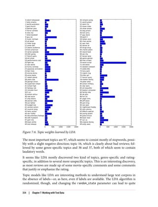
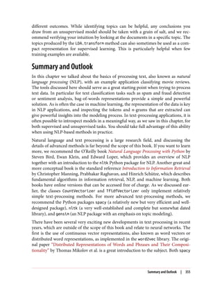
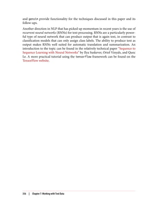
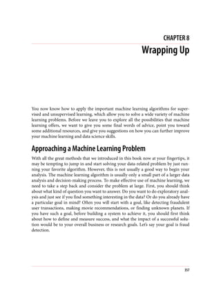
![In[1]:
from sklearn.base import BaseEstimator, TransformerMixin
class MyTransformer(BaseEstimator, TransformerMixin):
def __init__(self, first_parameter=1, second_parameter=2):
# All parameters must be specified in the __init__ function
self.first_parameter = 1
self.second_parameter = 2
def fit(self, X, y=None):
# fit should only take X and y as parameters
# Even if your model is unsupervised, you need to accept a y argument!
# Model fitting code goes here
print("fitting the model right here")
# fit returns self
return self
def transform(self, X):
# transform takes as parameter only X
# Apply some transformation to X
X_transformed = X + 1
return X_transformed
Implementing a classifier or regressor works similarly, only instead of Transformer
Mixin you need to inherit from ClassifierMixin or RegressorMixin. Also, instead
of implementing transform, you would implement predict.
As you can see from the example given here, implementing your own estimator
requires very little code, and most scikit-learn users build up a collection of cus‐
tom models over time.
Where to Go from Here
This book provides an introduction to machine learning and will make you an effec‐
tive practitioner. However, if you want to further your machine learning skills, here
are some suggestions of books and more specialized resources to investigate to dive
deeper.
Theory
In this book, we tried to provide an intuition of how the most common machine
learning algorithms work, without requiring a strong foundation in mathematics or
computer science. However, many of the models we discussed use principles from
probability theory, linear algebra, and optimization. While it is not necessary to
understand all the details of how these algorithms are implemented, we think that
Where to Go from Here | 361](https://image.slidesharecdn.com/introductiontomachinelearningwithpythonpdfdrive-230107170822-bfb01dbd/85/Introduction-to-Machine-Learning-with-Python-PDFDrive-com-pdf-375-320.jpg)