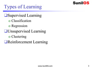
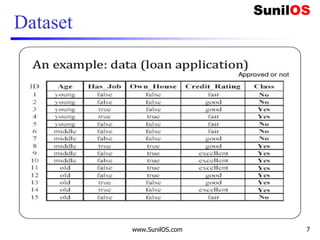
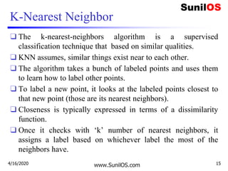
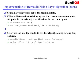
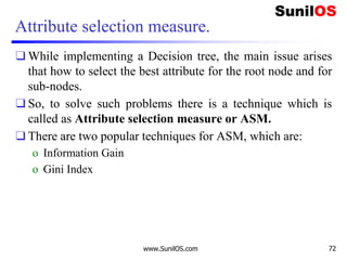
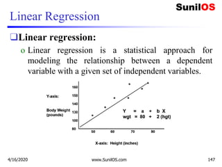
![Code implementation in scikit learn
❑ # Assigning features and label variables
❑ # First Feature
❑ weather=['Sunny','Sunny','Overcast','Rainy','Rainy',
'Rainy','Overcast','Sunny','Sunny',
❑ 'Rainy','Sunny','Overcast','Overcast','Rainy']
❑ # Second Feature
❑ temp=['Hot','Hot','Hot','Mild','Cool','Cool','Cool',
'Mild','Cool','Mild','Mild','Mild','Hot','Mild']
❑
❑ # Label or target variable
❑ play=['No','No','Yes','Yes','Yes','No','Yes','No','Y
es','Yes','Yes','Yes','Yes','No']
4/16/2020 www.SunilOS.com 21](https://image.slidesharecdn.com/machinelearningpart2-201121080138/85/Machine-learning-Part-2-21-320.jpg)
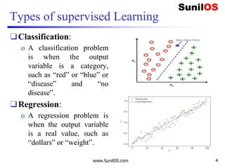
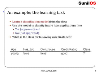
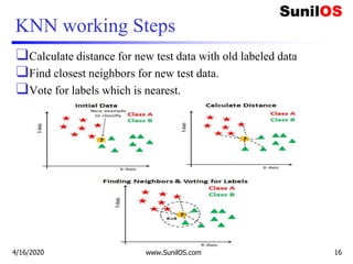
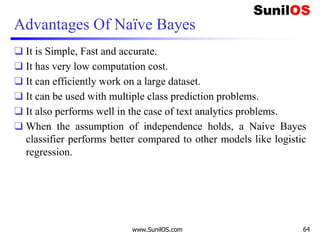
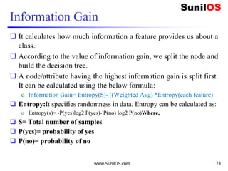
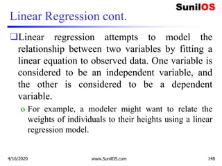
![Code implementation in scikit learn(cont.)
❑ #combining weather and temp into single list of tuples
❑ features=list(zip(weather_encoded,temp_encoded))
❑ print(features)
❑ #Prepare Model instance
❑ from sklearn.neighbors import KNeighborsClassifier
❑ model = KNeighborsClassifier(n_neighbors=3)
❑ # Train the model using the training sets
❑ model.fit(features,label)
❑ #Predict Output
❑ predicted= model.predict([[0,2]]) # 0:Overcast, 2:Mild
❑ print(predicted)
4/16/2020 www.SunilOS.com 23](https://image.slidesharecdn.com/machinelearningpart2-201121080138/85/Machine-learning-Part-2-23-320.jpg)
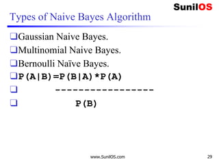

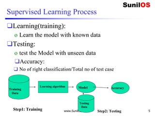
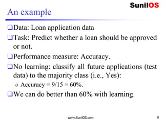
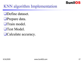
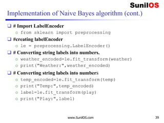
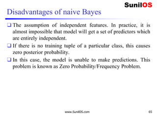
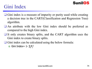
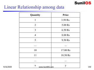
![Implementation of Naive Bayes algorithm:
❑ # Assigning features and label variables
❑ weather=['Sunny','Sunny','Overcast','Rainy','Ra
iny','Rainy','Overcast','Sunny','Sunny','Rainy'
,'Sunny','Overcast','Overcast','Rainy']
❑ temp=['Hot','Hot','Hot','Mild','Cool','Cool','C
ool','Mild','Cool','Mild','Mild','Mild','Hot','
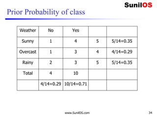
Mild']
❑ play=['No','No','Yes','Yes','Yes','No','Yes','N
o','Yes','Yes','Yes','Yes','Yes','No']
www.SunilOS.com 38](https://image.slidesharecdn.com/machinelearningpart2-201121080138/85/Machine-learning-Part-2-38-320.jpg)
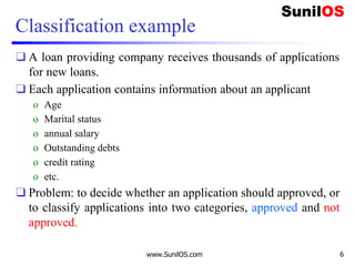
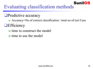
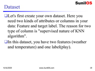
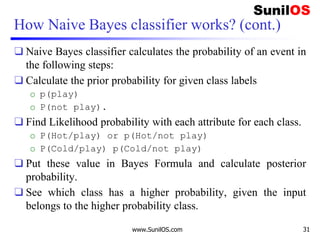
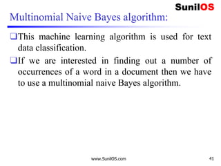
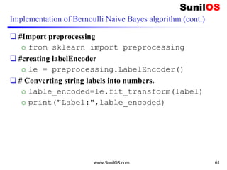
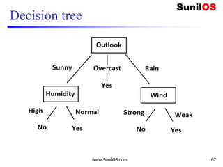
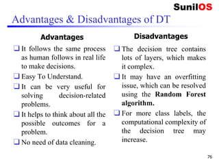
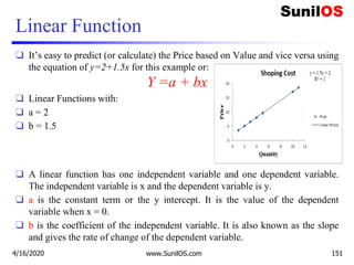
![Implementation of Naive Bayes algorithm (cont.)
❑ #Combining weather and temp into single list of tuples
o features=list(zip(weather_encoded,temp_encoded))
o print("Features:",features)
❑ #Import Gaussian Naive Bayes model
o from sklearn.naive_bayes import GaussianNB
❑ #Create a Gaussian Classifier
o model = GaussianNB()
❑ # Train the model using the training sets
o model.fit(features,label)
❑#Predict Output: 0:Overcast, 2:Mild
o predicted= model.predict([[0,2]])
o print ("Predicted Value:", predicted)
www.SunilOS.com 40](https://image.slidesharecdn.com/machinelearningpart2-201121080138/85/Machine-learning-Part-2-40-320.jpg)
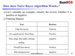


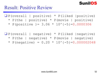
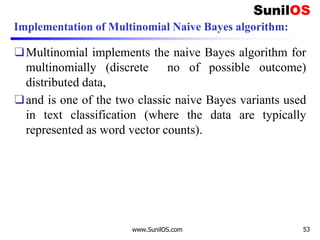
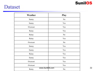
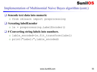
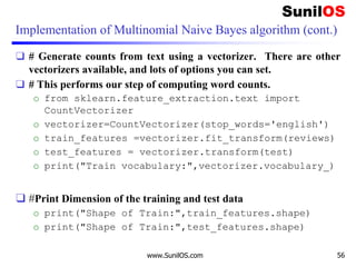
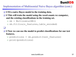
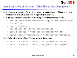
![Implementation of Multinomial Naive Bayes algorithm:
❑ # Assigning features and label variables
o import numpy as np
o reviews=np.array(['I like the movie',
o 'Its a good movie. Nice Story',
o 'Nice songs. But sadly a boring ending.',
o 'Overall nice movie',
o 'Sad, boring movie'])
o label=["positive","positive","negative","positive
","negative"]
o test=np.array(["Overall i like the movie"])
www.SunilOS.com 54](https://image.slidesharecdn.com/machinelearningpart2-201121080138/85/Machine-learning-Part-2-54-320.jpg)
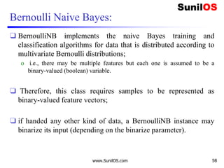

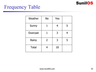
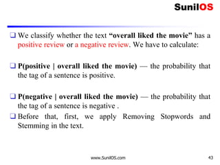
![Implementation of Bernoulli Naive Bayes algorithm (cont.)
❑ # Assigning features and label variables
o import numpy as np
o document=np.array(["Saturn Dealer’s Car",
o "Toyota Car Tercel",
o "Baseball Game Play",
o "Pulled Muscle Game",
o "Colored GIFs Root"])
o label=np.array(["Auto","Auto","Sports","Sports","
Computer"])
o test=np.array(["Home Runs Game","Car Engine
Noises"])
www.SunilOS.com 60](https://image.slidesharecdn.com/machinelearningpart2-201121080138/85/Machine-learning-Part-2-60-320.jpg)


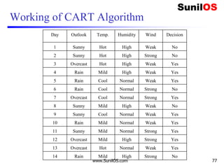


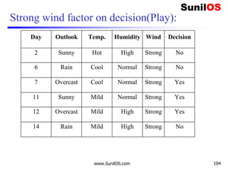
![Code Implementation of CART
❑ #Assigning features and label variables
❑ weather=['Sunny','Sunny','Overcast','Rainy','Rainy',
'Rainy','Overcast','Sunny','Sunny','Rainy','Sunny',
'Overcast', 'Overcast‘ , 'Rainy']
❑
❑ temp=['Hot','Hot','Hot','Mild','Cool','Cool','Cool',
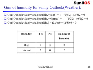
'Mild','Cool','Mild','Mild','Mild','Hot','Mild']
❑
❑ humidity=["High","High","High","High","Normal","Norm
al","Normal","High","Normal","Normal","Normal","High
","Normal","High"]
❑
❑ Windy=["Weak","Strong","Weak","Weak","Weak","Strong“
,"Strong","Weak","Weak","Weak","Strong","Strong","We
ak","Strong"]
www.SunilOS.com 95](https://image.slidesharecdn.com/machinelearningpart2-201121080138/85/Machine-learning-Part-2-95-320.jpg)
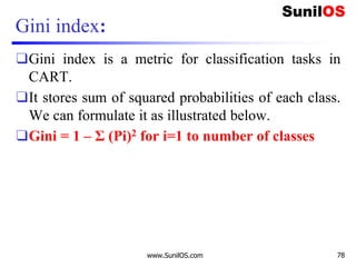
![Code Implementation of CART
❑ play=['No','No','Yes','Yes','Yes','No','Yes','N
o','Yes','Yes','Yes','Yes','Yes','No']
❑
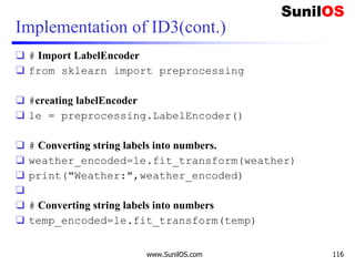
❑ # Import LabelEncoder
❑ from sklearn import preprocessing
❑
❑ #creating labelEncoder
❑ le = preprocessing.LabelEncoder()
❑
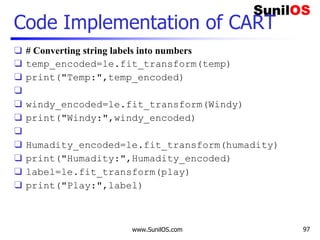
❑ # Converting string labels into numbers.
❑ weather_encoded=le.fit_transform(weather)
❑ print("Weather:",weather_encoded)
❑
www.SunilOS.com 96](https://image.slidesharecdn.com/machinelearningpart2-201121080138/85/Machine-learning-Part-2-96-320.jpg)
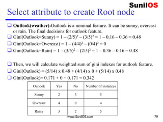
![Code Implementation of CART
❑ #Combinig weather,temp, Windy, humadity into single listof tuples
❑ features=list(zip(weather_encoded,temp_encoded,windy
_encoded,Humadity_encoded))
❑ print("Features:",features)
❑ #Import the DecisionTreeClassifier
❑ from sklearn.tree import DecisionTreeClassifier
❑ tree = DecisionTreeClassifier(criterion='gini')
❑ #Train the Model
❑ tree.fit(features,label)
❑ #Test Model 2:sunny, 2:Mild 0:Windy:Strong 0:Humadity:High
❑ prediction = tree.predict([[2,2,1,0]])
❑ print("Decision",prediction)
❑
www.SunilOS.com 98](https://image.slidesharecdn.com/machinelearningpart2-201121080138/85/Machine-learning-Part-2-98-320.jpg)
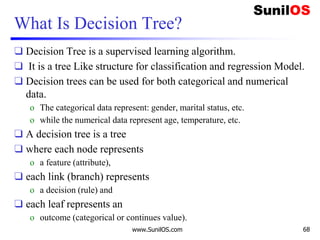
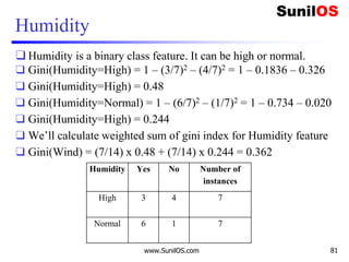
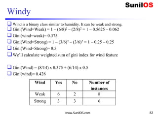
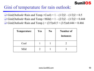
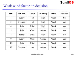
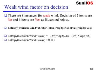
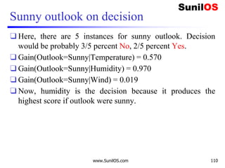
![Wind factor on decision
❑ Formula:
o Gain(Decision,Wind)=Entropy(Decision) – ∑ [ p(Decision|Wind).*
Entropy(Decision|Wind)]
❑ Wind attribute has two labels: Weak and Strong. We
would reflect it to the formula.
o Gain(Decision,Wind)=Entropy(Decision)–
[p(Decision|Wind=Weak)*Entropy(Decision|Wind=Weak)]-
[p(Decision|Wind=Strong)*Entropy(Decision|Wind=Strong) ]
❑ Now, we need to calculate (Decision|Wind=Weak)
and (Decision|Wind=Strong) respectively.
www.SunilOS.com 101](https://image.slidesharecdn.com/machinelearningpart2-201121080138/85/Machine-learning-Part-2-101-320.jpg)
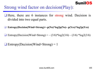
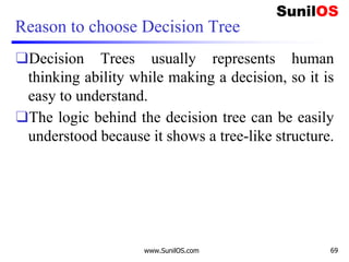
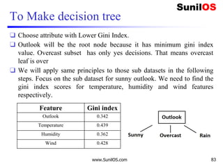
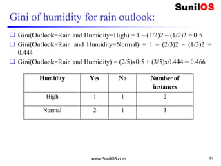
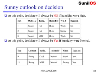
![Information Gain for Wind Attribute
❑ Formula:
o Gain(Decision,Wind) = Entropy(Decision)–
[p(Decision|Wind=Weak) * Entropy(Decision|Wind=Weak) ] –
[p(Decision|Wind=Strong)*Entropy(Decision|Wind=Strong) ]
❑ Gain(Decision,Wind) = 0.940 – [ (8/14) *0.811 ] – [ (6/14)*1]
❑ Gain(Decision,Wind) = 0.048
❑ We Have calculated Gain for Wind. Apply the same procedure to
Others to get Best attribute to make it root node.
www.SunilOS.com 106](https://image.slidesharecdn.com/machinelearningpart2-201121080138/85/Machine-learning-Part-2-106-320.jpg)

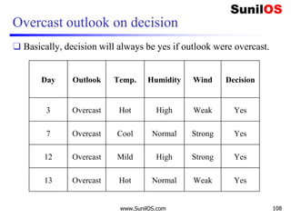


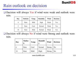
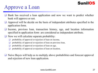
![Implementation of ID3
❑ #Import the DecisionTreeClassifier
❑ from sklearn.tree import DecisionTreeClassifier
❑ # Assigning features and label variables
❑ weather=['Sunny','Sunny','Overcast','Rainy','Ra
iny','Rainy','Overcast','Sunny','Sunny',
'Rainy','Sunny','Overcast','Overcast','Rainy']
❑ temp=['Hot','Hot','Hot','Mild','Cool','Cool','C
ool','Mild','Cool','Mild','Mild','Mild','Hot','
Mild']
❑
❑ play=['No','No','Yes','Yes','Yes','No','Yes','N
o','Yes','Yes','Yes','Yes','Yes','No']
www.SunilOS.com 115](https://image.slidesharecdn.com/machinelearningpart2-201121080138/85/Machine-learning-Part-2-115-320.jpg)
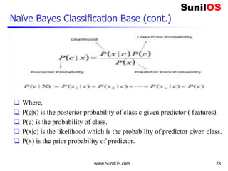
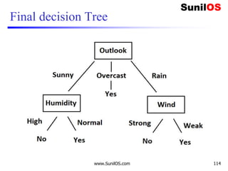
![Implementation of ID3(cont.)
❑ print("Temp:",temp_encoded)
❑ label=le.fit_transform(play)
❑ print("Play:",label)
❑ #Combinig weather and temp into single listof tuples
❑ features=list(zip(weather_encoded,temp_encoded))
❑ print("Features:",features)
❑ #Create Instance of Model, and train the model
❑ tree = DecisionTreeClassifier(criterion='entropy')
❑ tree.fit(features,label)
❑ #Predict result for 0:Overcast, 2:mild
❑ prediction = tree.predict([[0,2]])
❑ print("Decision",prediction)
www.SunilOS.com 117](https://image.slidesharecdn.com/machinelearningpart2-201121080138/85/Machine-learning-Part-2-117-320.jpg)

![Code implementation of random Forest
❑ #Assign features
❑ weather=['Sunny','Sunny','Overcast','Rainy'
,'Rainy','Rainy','Overcast','Sunny','Sunny'
,'Rainy','Sunny','Overcast','Overcast',
'Rainy']
❑ temp=['Hot','Hot','Hot','Mild','Cool','Cool
','Cool','Mild','Cool','Mild','Mild','Mild'
,'Hot','Mild']
❑ humadity=["High","High","High","High","Norm
al","Normal","Normal","High","Normal","Norm
al","Normal","High", "Normal","High"]
www.SunilOS.com 122](https://image.slidesharecdn.com/machinelearningpart2-201121080138/85/Machine-learning-Part-2-122-320.jpg)
![Code implementation of random Forest
❑ Windy=["Weak","Strong","Weak","Weak","Weak"
,"Strong","Strong","Weak","Weak","Weak",
"Strong","Strong","Weak","Strong"]
❑ play=['No','No','Yes','Yes','Yes','No','Yes
','No','Yes','Yes','Yes','Yes','Yes','No']
❑
❑ #Import LabelEncoder
❑ from sklearn import preprocessing
❑ #creating labelEncoder
❑ le = preprocessing.LabelEncoder()
www.SunilOS.com 123](https://image.slidesharecdn.com/machinelearningpart2-201121080138/85/Machine-learning-Part-2-123-320.jpg)
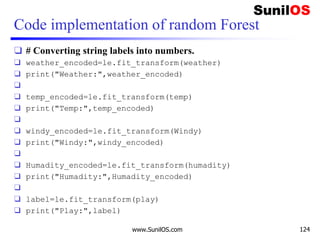
![Code implementation of random Forest
❑ #Combinig weather and temp into single listof tuples
❑ features=list(zip(weather_encoded,temp_encoded,
❑ windy_encoded,Humadity_encoded))
❑ #Import the RandomforestClassifier
❑ from sklearn.ensemble import RandomForestClassifi
er
❑ #create instance of the Random Forest Classifier
❑ tree= RandomForestClassifier(n_estimators=5)
❑ #train the Model
❑ tree.fit(features,label)
❑ #Test 2:sunny, 2:Mild 0:Windy:Strong 0:Humadity:High
❑ prediction = tree.predict([[2,2,1,0]])
❑ print("Decision",prediction)
www.SunilOS.com 125](https://image.slidesharecdn.com/machinelearningpart2-201121080138/85/Machine-learning-Part-2-125-320.jpg)

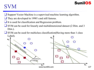


![Implementation of Linear SVM:
❑ #import liabraries
❑ import numpy as np
❑ import matplotlib.pyplot as plt
❑ from matplotlib import style
❑ style.use("ggplot")
❑ from sklearn import svm
❑ #Attributes
❑ x = [1, 5, 1.5, 8, 1, 9]
❑ y = [2, 8, 1.8, 8, 0.6,11]
❑ plt.scatter(x,y)
❑ plt.show()
www.SunilOS.com 131](https://image.slidesharecdn.com/machinelearningpart2-201121080138/85/Machine-learning-Part-2-131-320.jpg)
![Implementation of Linear SVM(cont.)
❑ #import preprocessing
❑ from sklearn import preprocessing
❑ X=list(zip(x,y))
❑ y = [0,1,0,1,0,1]
❑ #Train SVM Model
❑ clf = svm.SVC(kernel='linear', C = 1.0)
❑ clf.fit(X,y)
❑ # Test x=0.58, y=0.76
❑ print(clf.predict([[0.58,0.76]]))
❑ #x=10.58, y=10.76
❑ print(clf.predict([[10.58,10.76]]))
www.SunilOS.com 132](https://image.slidesharecdn.com/machinelearningpart2-201121080138/85/Machine-learning-Part-2-132-320.jpg)

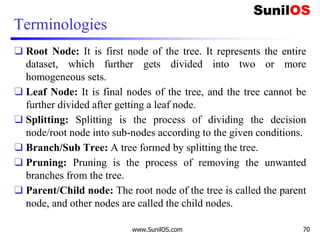
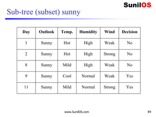
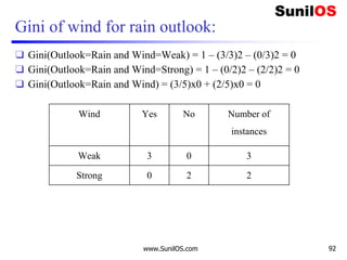
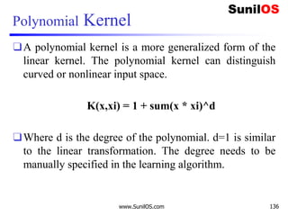
![Linear Kernel
❑A linear kernel can be used as normal dot product any two given
observations. The product between two vectors is the sum of the
multiplication of each pair of input values.
o K(x, xi) = sum(x * xi)
❑ For example, the inner product of the vectors [1, 2] and [3, 4] is 1*3 + 2*4 or
11.
❑ The equation for making a prediction for a new input using the dot product
between the input (x) and each support vector (xi) is calculated as follows:
f(x) = B0 + sum(ai * (x,xi))
❑ This is an equation that is used for calculating the inner products of a new
input vector (x) with all support vectors in training data. The coefficients B0
and ai (for each input) must be estimated from the training data by the learning
algorithm.
www.SunilOS.com 135](https://image.slidesharecdn.com/machinelearningpart2-201121080138/85/Machine-learning-Part-2-135-320.jpg)
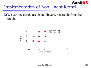
![Implementation of Non Linear Kernel
❑ # Assigning features and label variables
❑ weather=['Sunny','Sunny','Overcast','Rainy','Ra
iny','Rainy','Overcast','Sunny','Sunny','Rainy'
,'Sunny','Overcast','Overcast','Rainy']
❑
❑ temp=['Hot','Hot','Hot','Mild','Cool','Cool','C
ool','Mild','Cool','Mild','Mild','Mild','Hot','
Mild']
❑
❑ humadity=["High","High","High","High","Normal",
"Normal","Normal","High","Normal","Normal","Nor
mal","High","Normal","High"]
❑
www.SunilOS.com 139](https://image.slidesharecdn.com/machinelearningpart2-201121080138/85/Machine-learning-Part-2-139-320.jpg)
![Implementation of Non Linear Kernel
❑ Windy=["Weak","Strong","Weak","Weak","Weak","St
rong","Strong","Weak","Weak","Weak","Strong","S
trong","Weak","Strong"]
❑
❑ play=['No','No','Yes','Yes','Yes','No','Yes','N
o','Yes','Yes','Yes','Yes','Yes','No']
❑ # Import LabelEncoder
❑ from sklearn import preprocessing
❑ #creating labelEncoder
❑ le = preprocessing.LabelEncoder()
❑ # Converting string labels into numbers.
❑ weather_encoded=le.fit_transform(weather)
❑ print("Weather:",weather_encoded)
www.SunilOS.com 140](https://image.slidesharecdn.com/machinelearningpart2-201121080138/85/Machine-learning-Part-2-140-320.jpg)
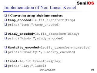
![Implementation of Non Linear Kernel
❑ #Combinig weather and temp into single list of tuples
❑ features=list(zip(weather_encoded,temp_encoded,windy
_encoded,Humadity_encoded))
❑ print("Features:",features)
❑ #import svm
❑ from sklearn import svm
❑ #Create a svm Classifier
❑ clf = svm.SVC(kernel='rbf') # Linear Kernel
❑ #Train SVM Model
❑ clf.fit(features,label)
❑ # Test 2:sunny, 2:Mild 0:Windy:Strong 0:Humadity:High
❑ prediction = clf.predict([[2,2,1,0]])
❑ print("Decision",prediction)
www.SunilOS.com 142](https://image.slidesharecdn.com/machinelearningpart2-201121080138/85/Machine-learning-Part-2-142-320.jpg)

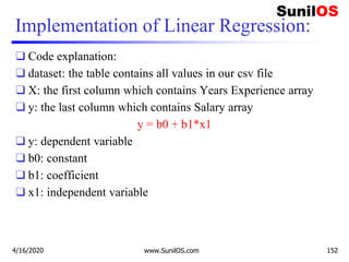
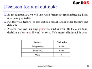
![Code Implementation of Linear Regression
❑ import numpy as np
❑ import matplotlib.pyplot as plt
❑ import pandas as pd
❑ # Importing the dataset
❑ dataset=pd.read_csv('E:/MLImplementation/r
egression.csv')
❑ #get a copy of dataset exclude last column
❑ X = dataset.iloc[:, :-1].values
❑ #get array of dataset in column 1st
❑ y = dataset.iloc[:, 1].values
4/16/2020 www.SunilOS.com 155](https://image.slidesharecdn.com/machinelearningpart2-201121080138/85/Machine-learning-Part-2-155-320.jpg)

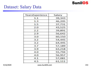
![Code Implementation of Linear Regression (cont.)
❑ # Predicting the Test set results
❑ y_pred = regressor.predict(X_test)
❑ #predicting the salary for 5 year Experienced Employee
❑ y_pred = regressor.predict([[5]])
❑ print(y_pred)
4/16/2020 www.SunilOS.com 157](https://image.slidesharecdn.com/machinelearningpart2-201121080138/85/Machine-learning-Part-2-157-320.jpg)
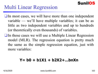
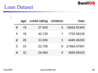
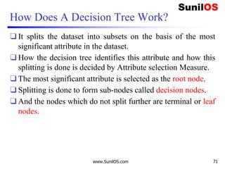
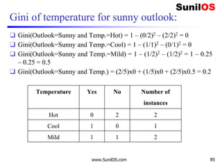
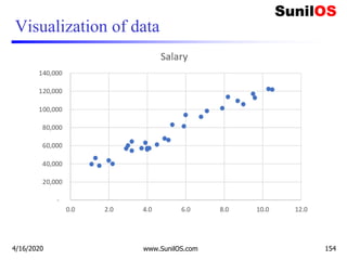
![Code Implementation of MLR
❑ #Features age, credit-rating and no of children
❑ age=[19,18,28,33,32,31,46,37,37,60,25,62,23,56]
❑ credit_rating=[27.9,42.13,33,22.705,28.88,25.74,
❑ 33.44,27.74,29.83,25.84,26.22,26.29,34.4,39.82]
❑ children=[0,1,3,0,0,0,1,3,2,0,0,0,0,0]
❑ #Label data
❑ loan=[16884.924,1725.5523,4449.462,21984.47061,3866.
8552,
❑ 3756.6216,8240.5896,7281.5056,6406.4107,28923.13692,
❑ 2721.3208,27808.7251,1826.843,11090.7178,]
4/16/2020 www.SunilOS.com 167](https://image.slidesharecdn.com/machinelearningpart2-201121080138/85/Machine-learning-Part-2-167-320.jpg)
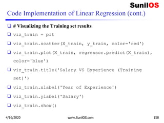
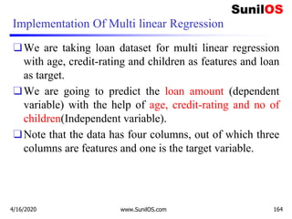
![Code Implementation of MLR (cont.)
❑ #Combining age, credit-rating and children into single list of tuples
❑ features=list(zip(age,credit_rating,children))
❑ print(features)
❑ #define the multiple Linear regression model
❑ linear_regress = LinearRegression()
❑ #Fit the multiple Linear regression model
❑ linear_regress.fit(features,loan)
❑ print("coefficient:",linear_regress.coef_)
❑ print("intercept:",linear_regress.intercept_)
❑ # predict with test data
❑ #age:20,credit-rating:32,children:0
❑ y_pred=linear_regress.predict([[20,32,0]])
❑ print(y_pred)
4/16/2020 www.SunilOS.com 168](https://image.slidesharecdn.com/machinelearningpart2-201121080138/85/Machine-learning-Part-2-168-320.jpg)


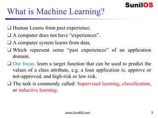
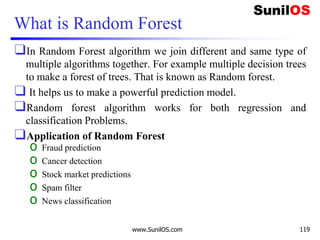
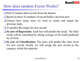
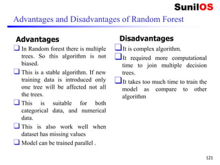
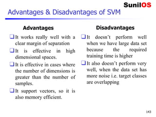
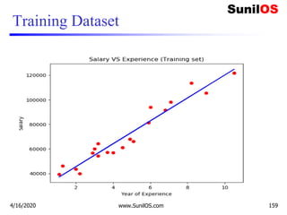
Supervised learning involves using a training dataset to learn a target function that can be used to predict class labels or attribute values. The document discusses supervised learning and classification, including types of supervised learning problems like classification and regression. It provides examples of classification algorithms like K-nearest neighbors, decision trees, naive Bayes, and support vector machines. It also gives examples of how to implement classification algorithms using scikit-learn and discusses evaluating classification model performance based on accuracy.