Downloaded 150 times
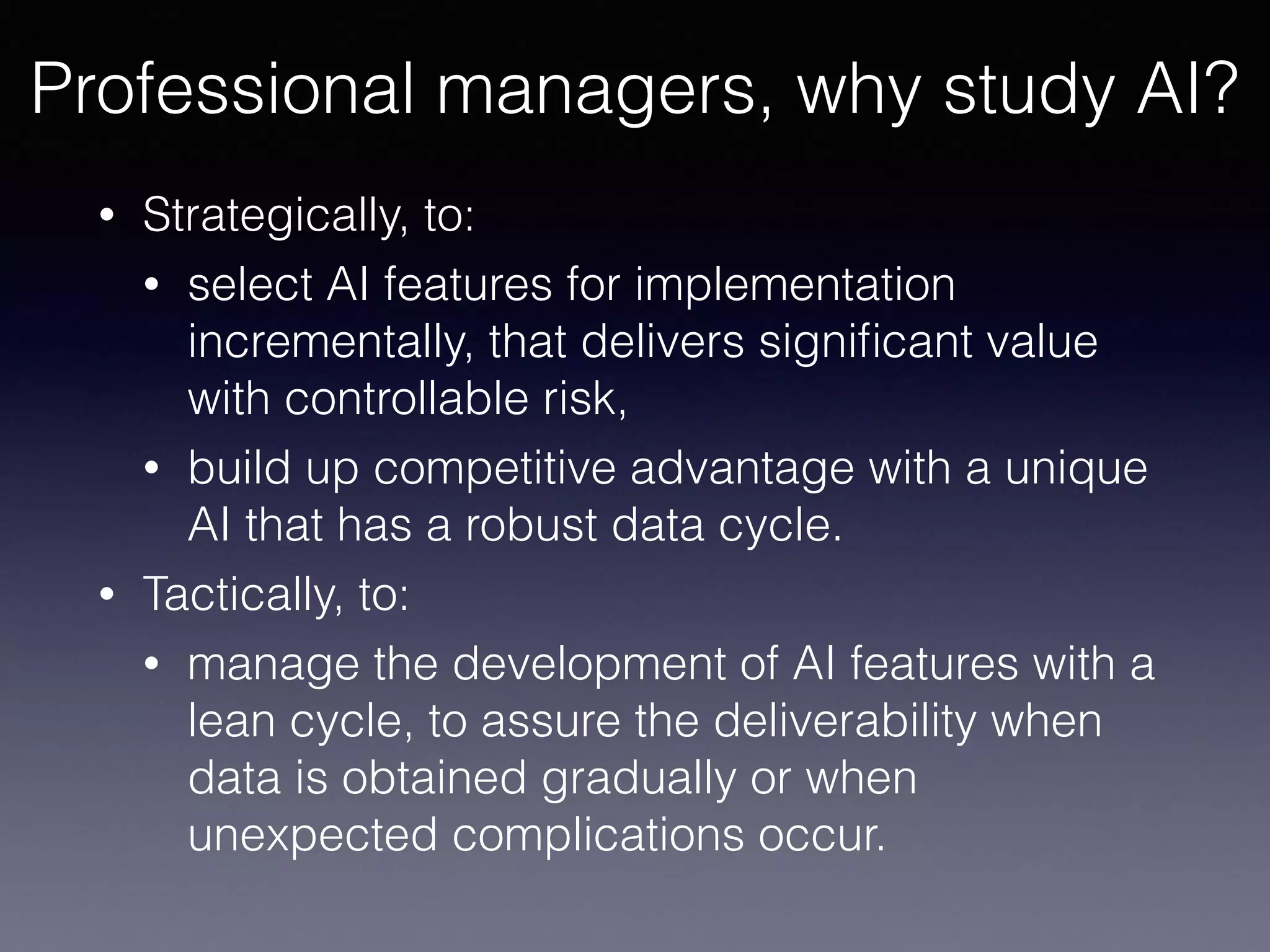
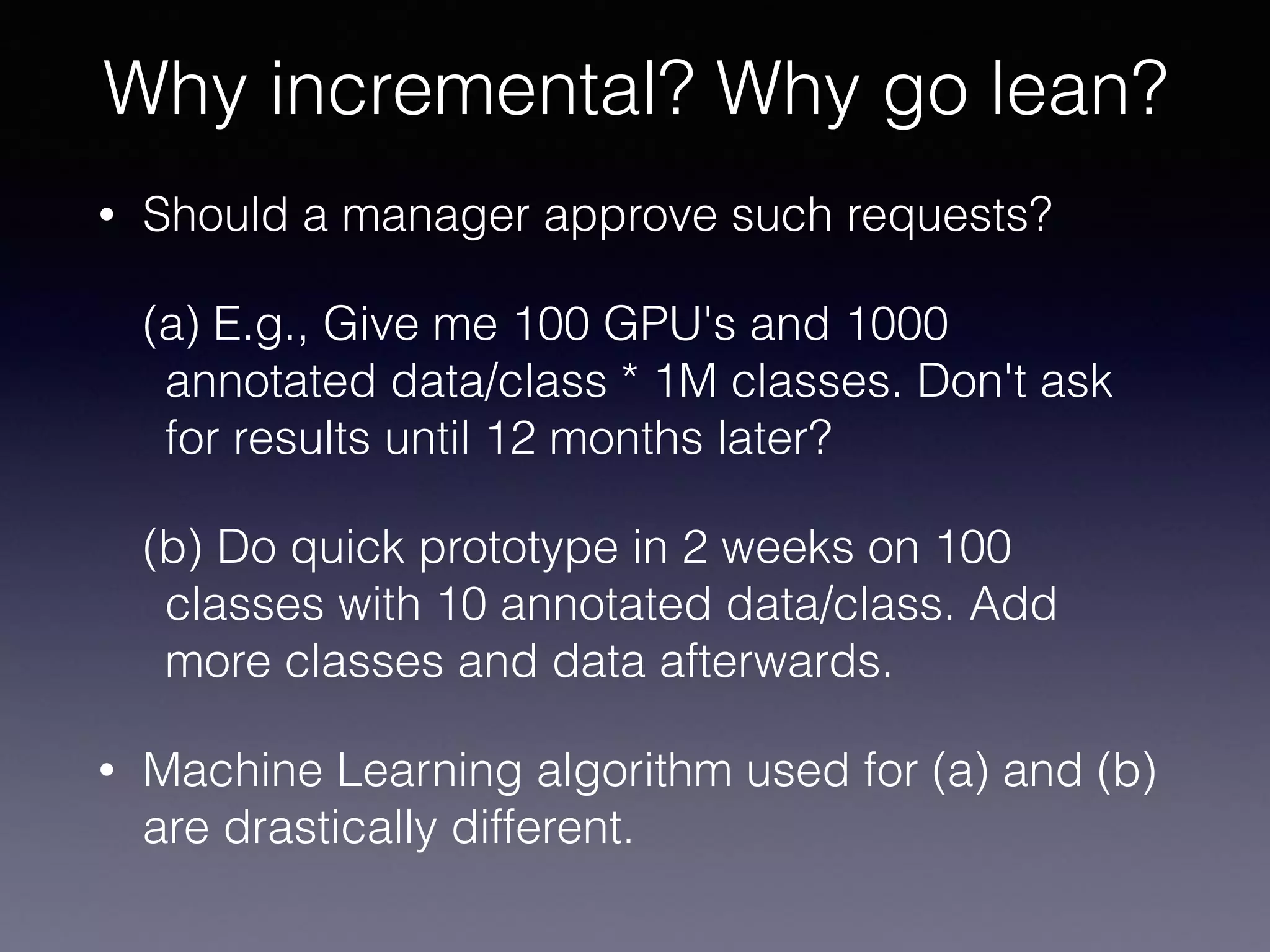
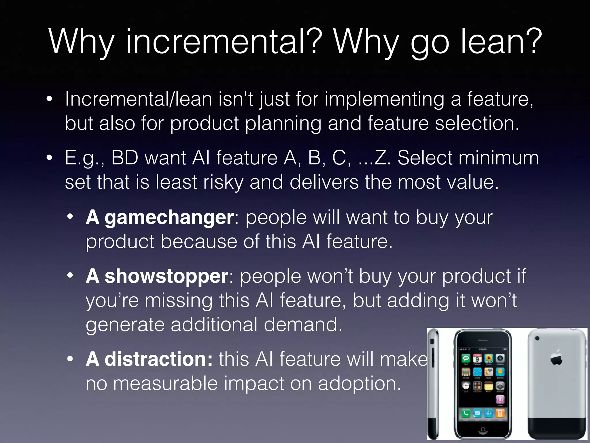
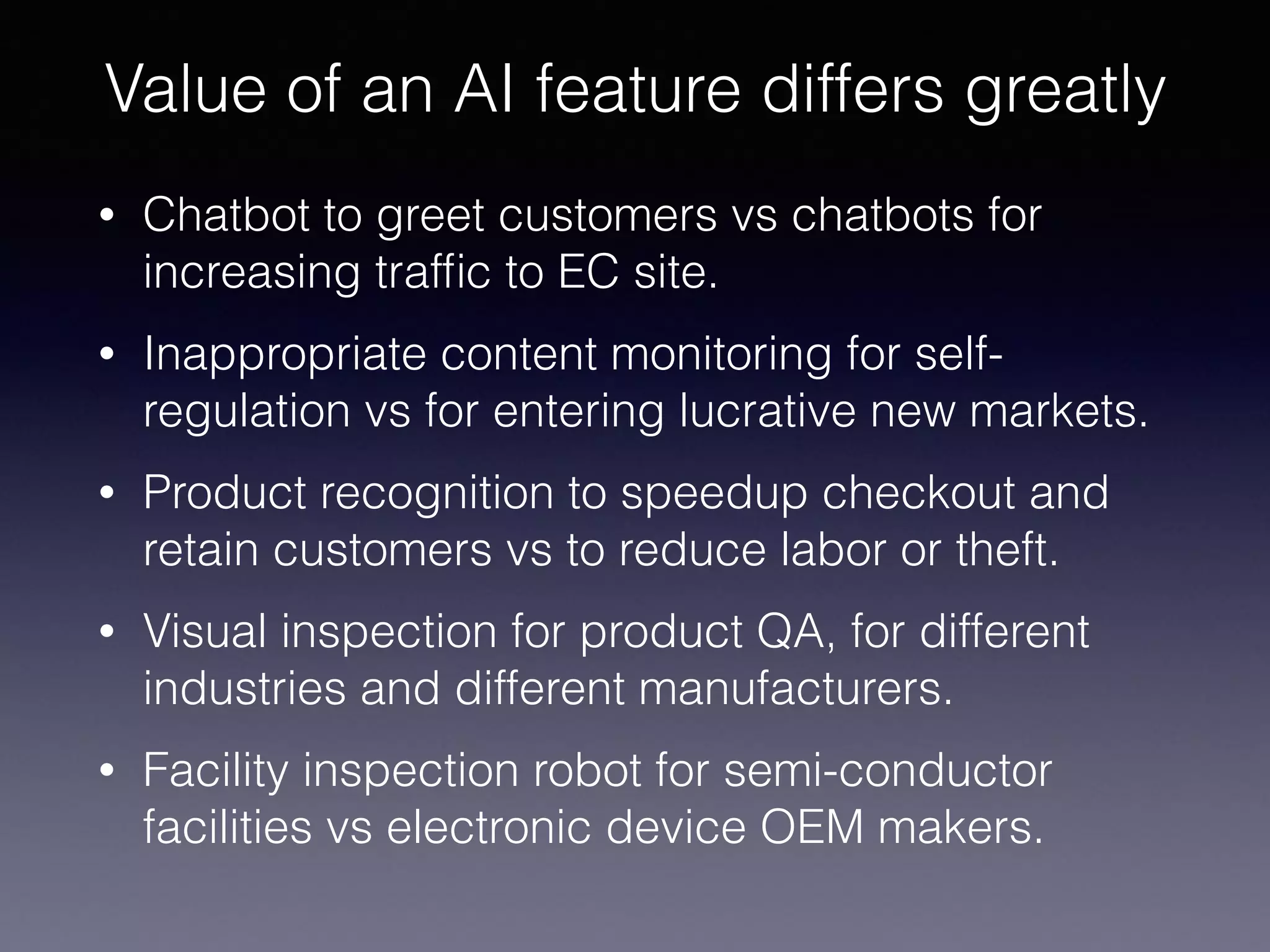
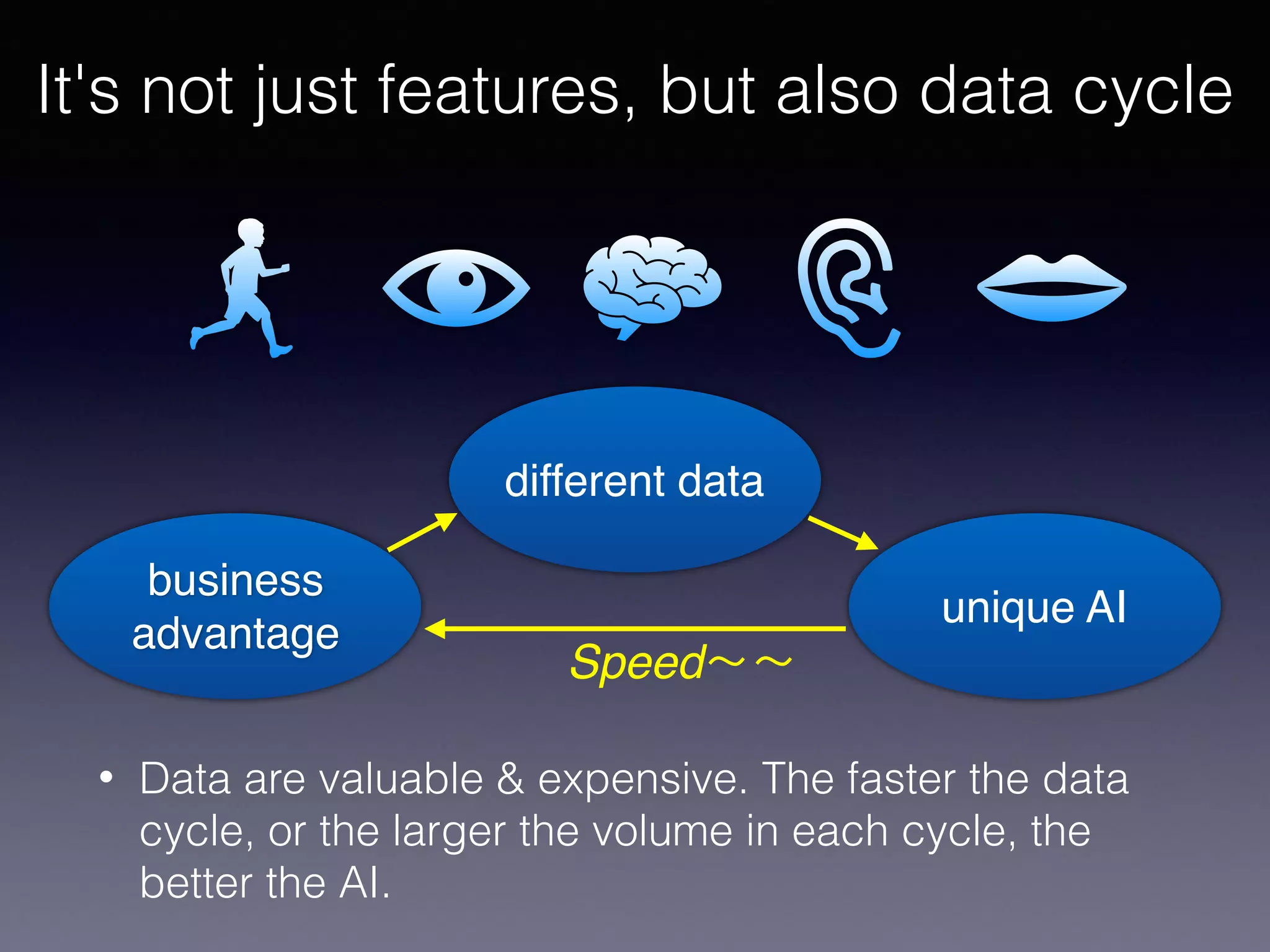
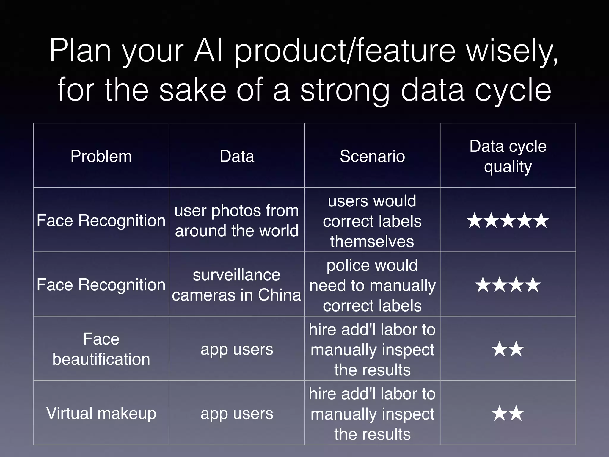
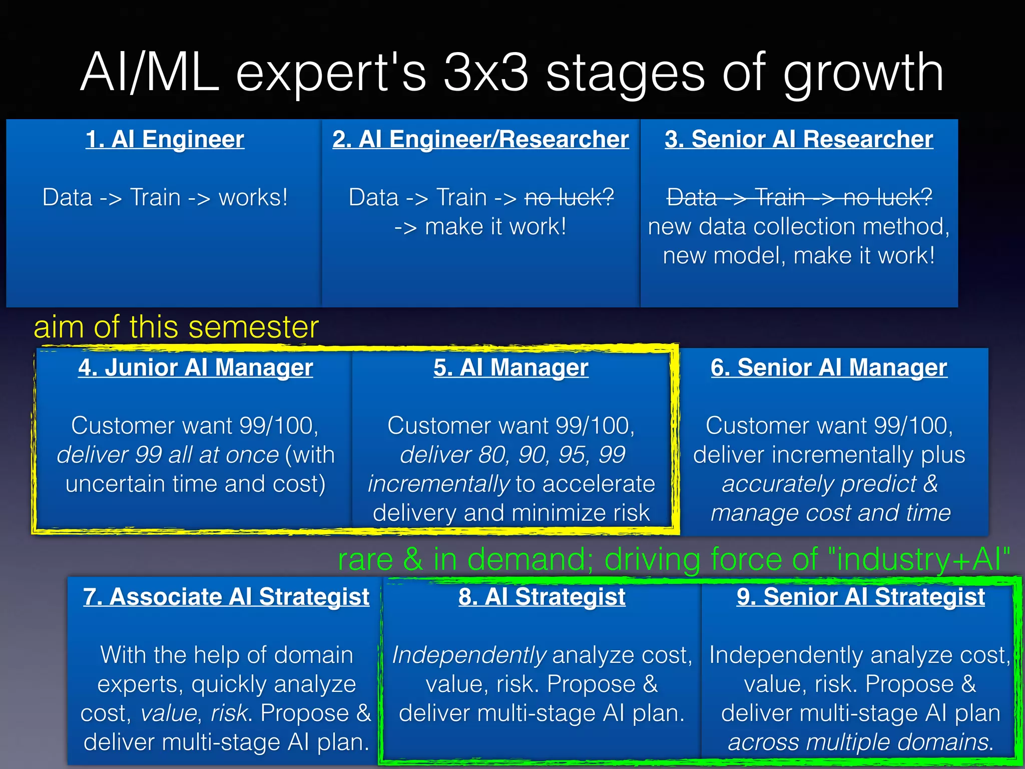
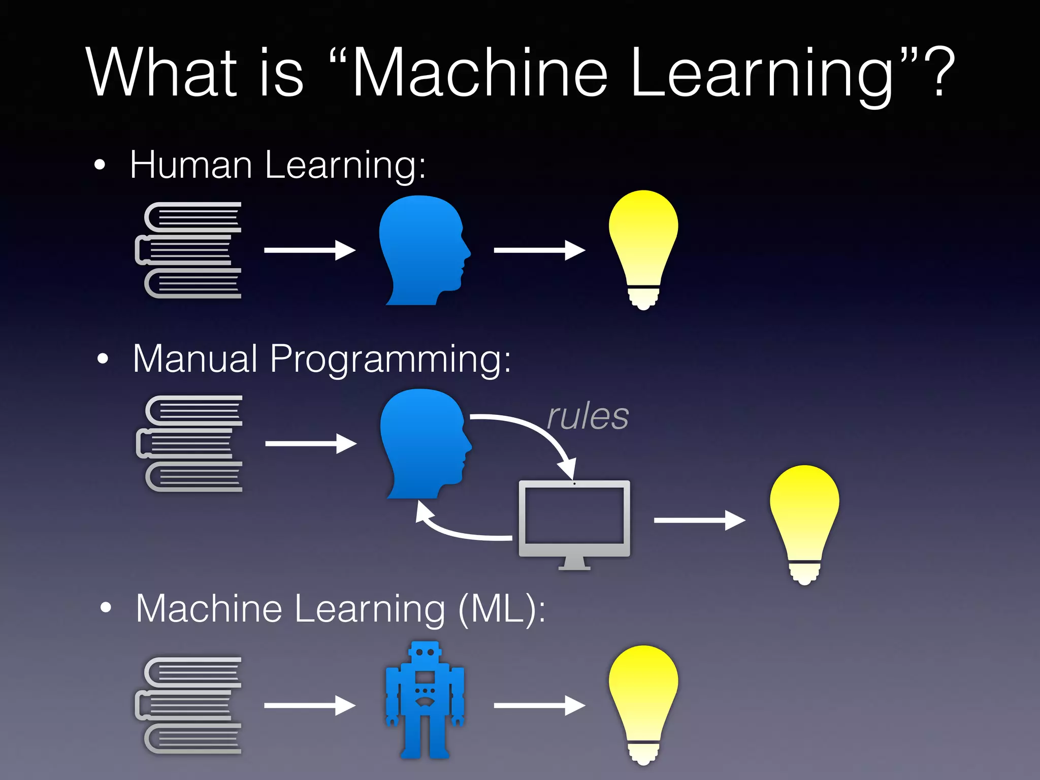
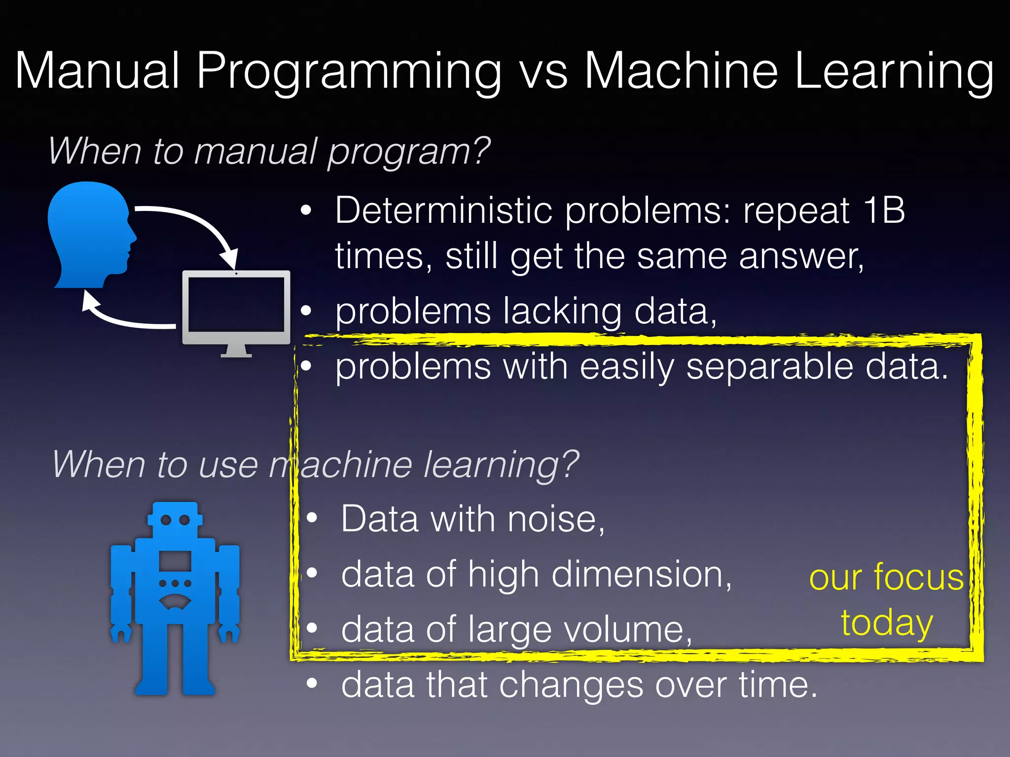
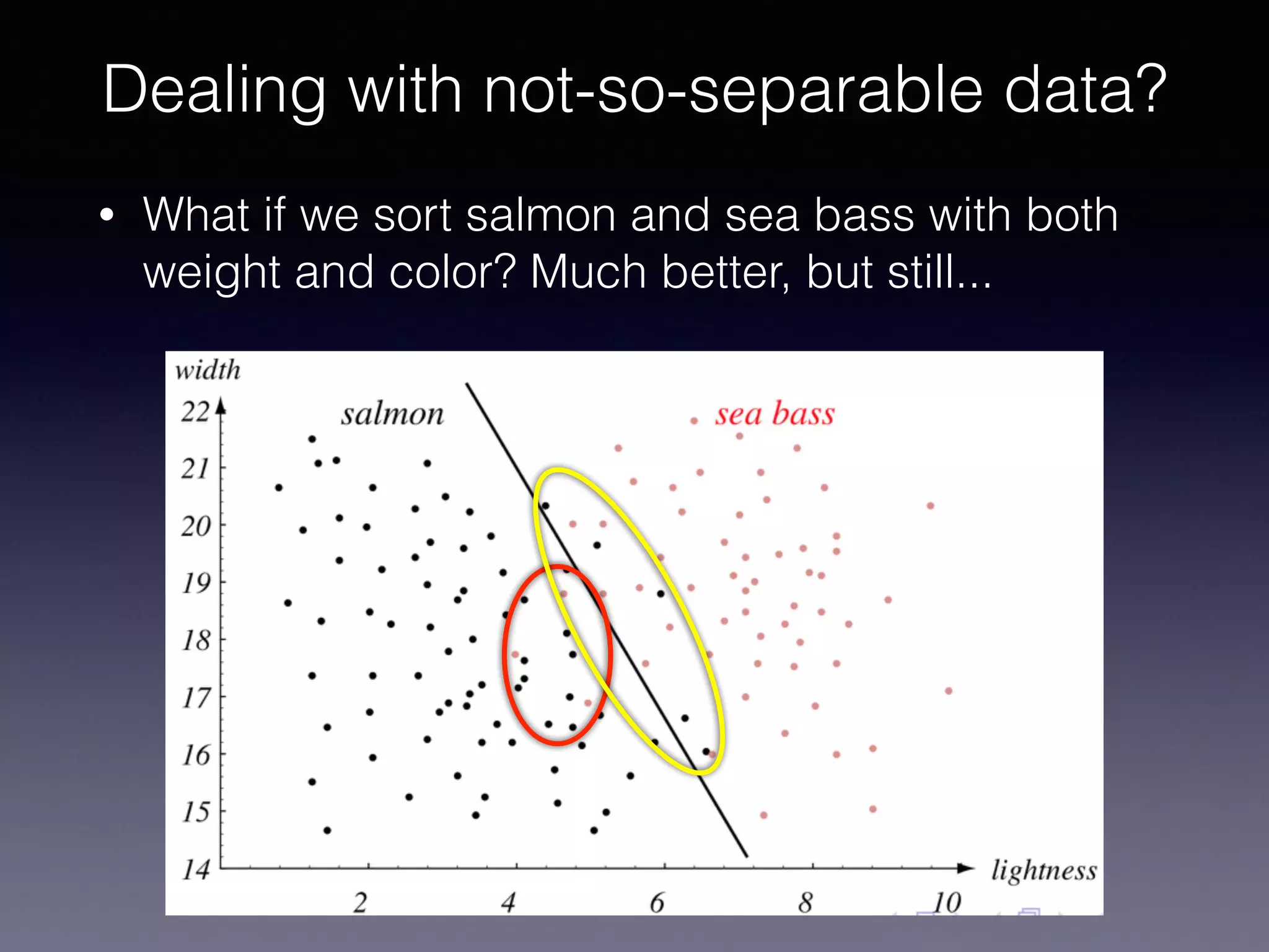
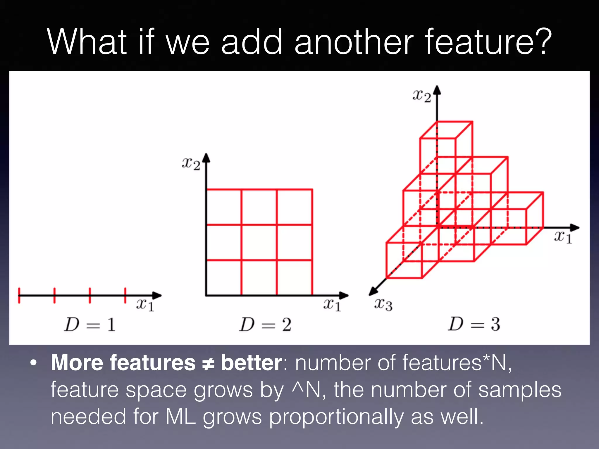

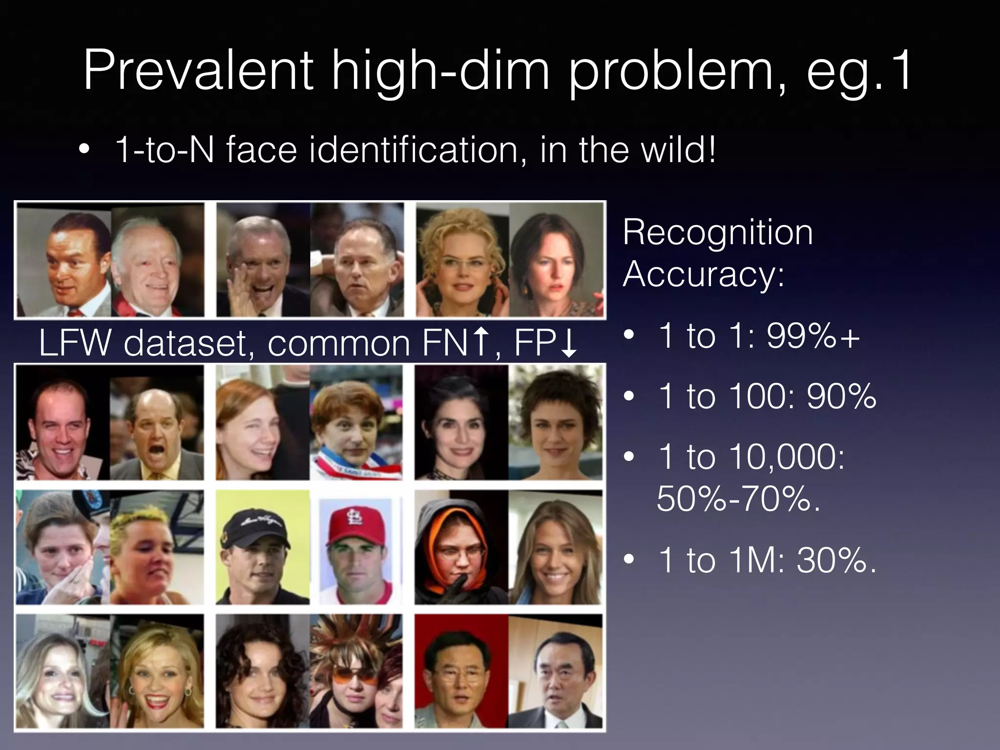
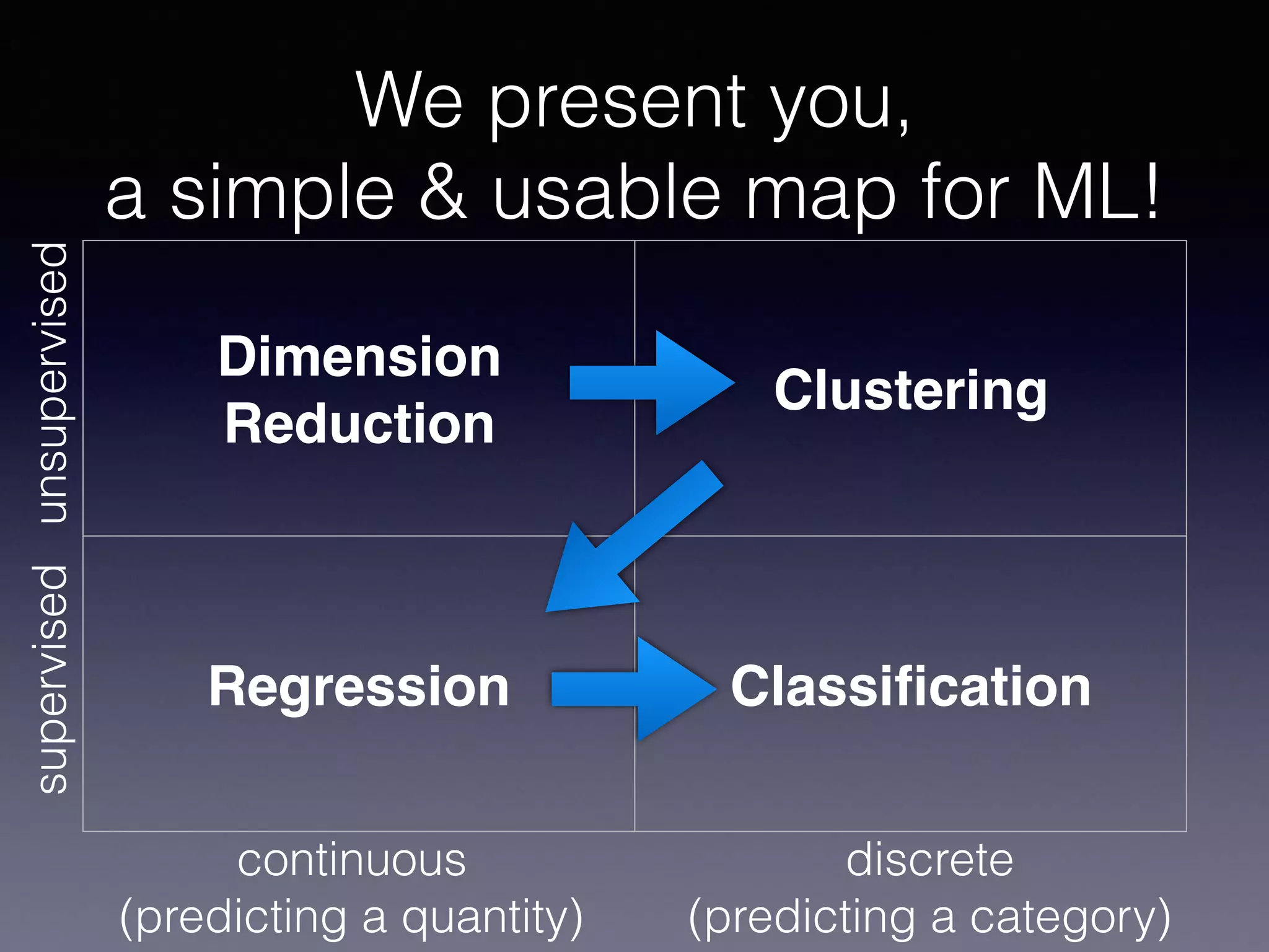
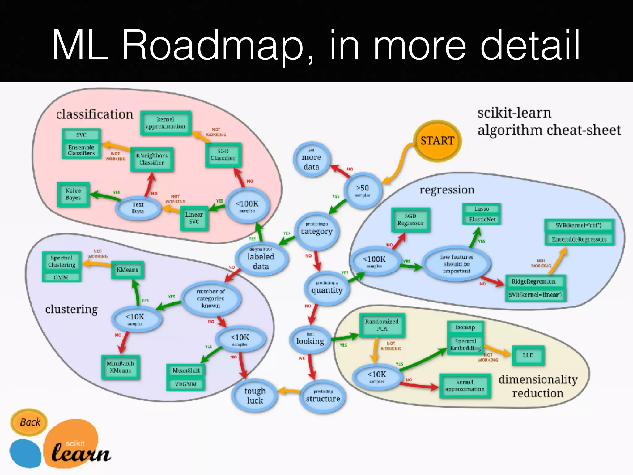
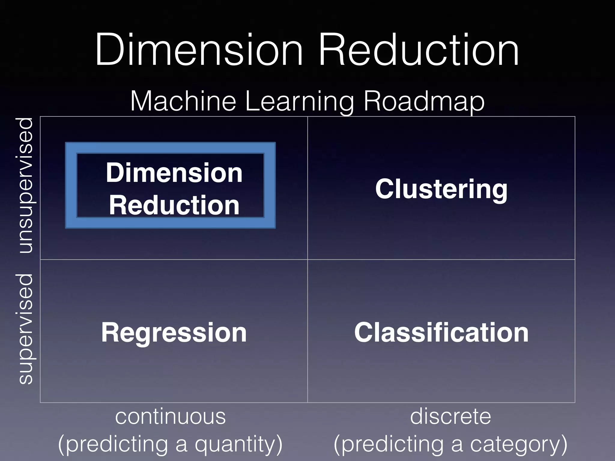
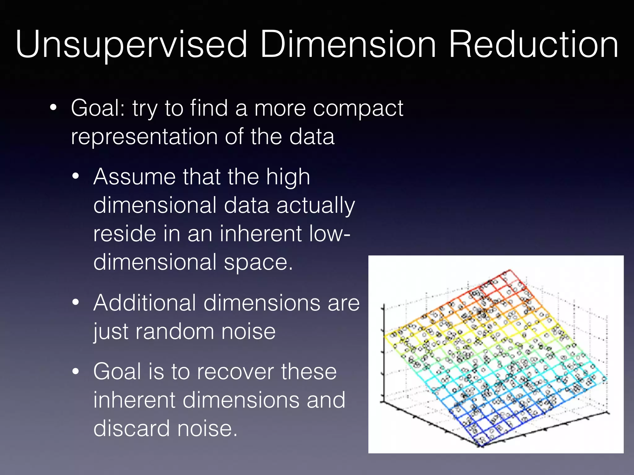
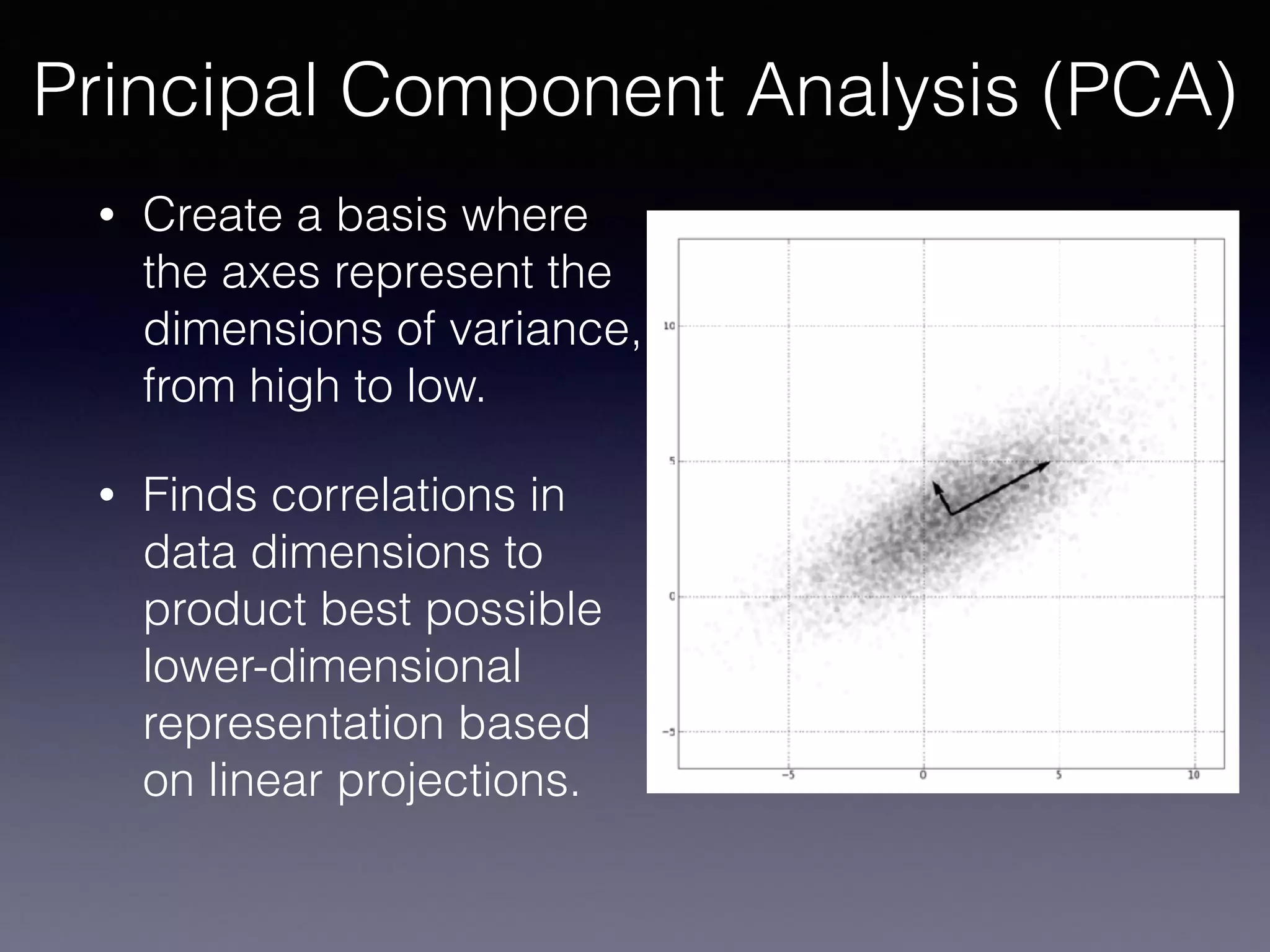
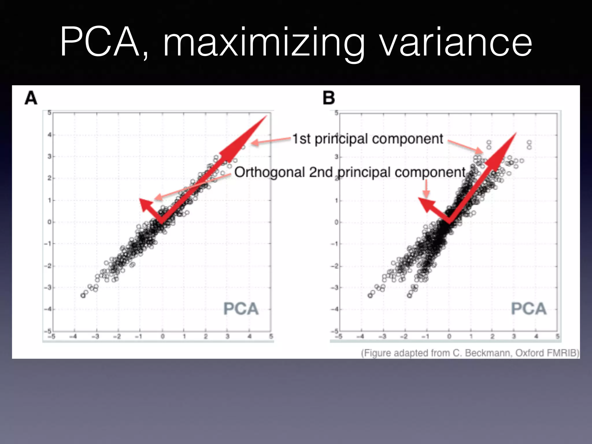
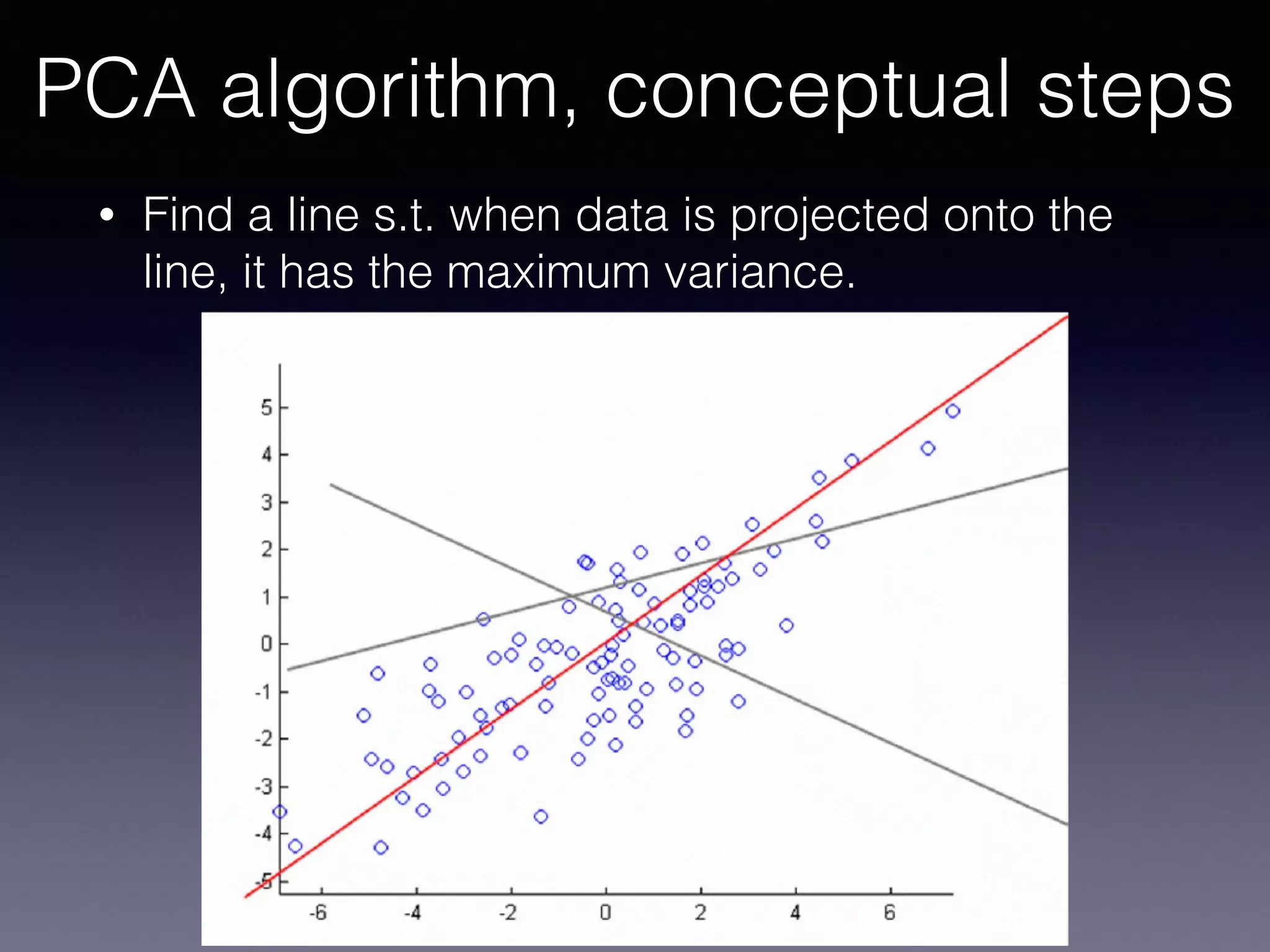
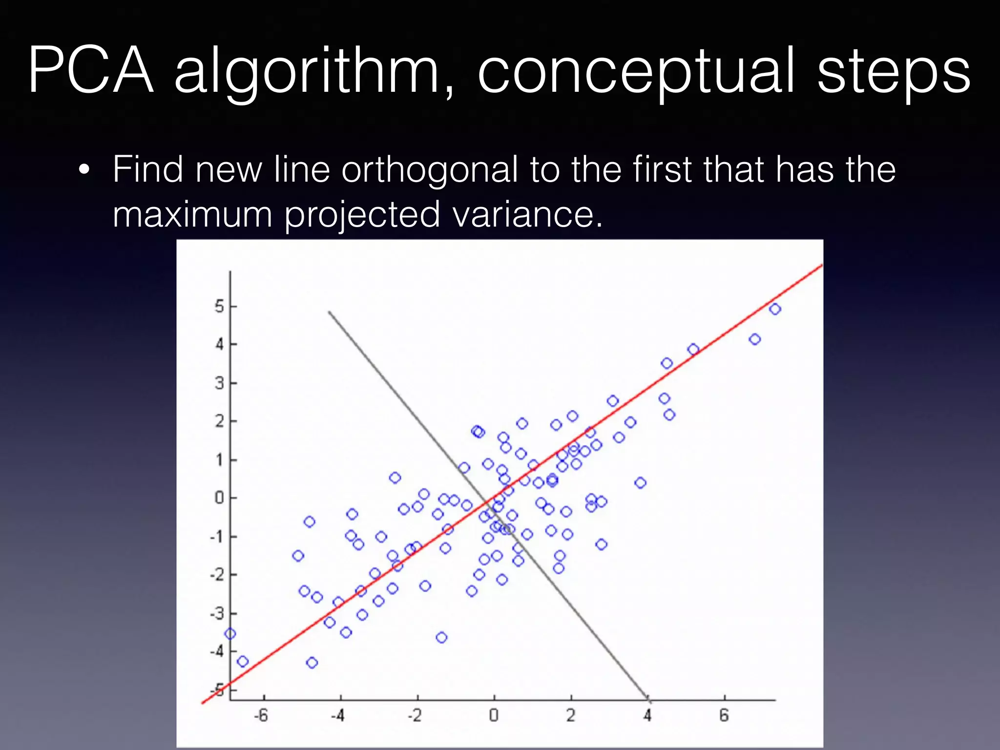

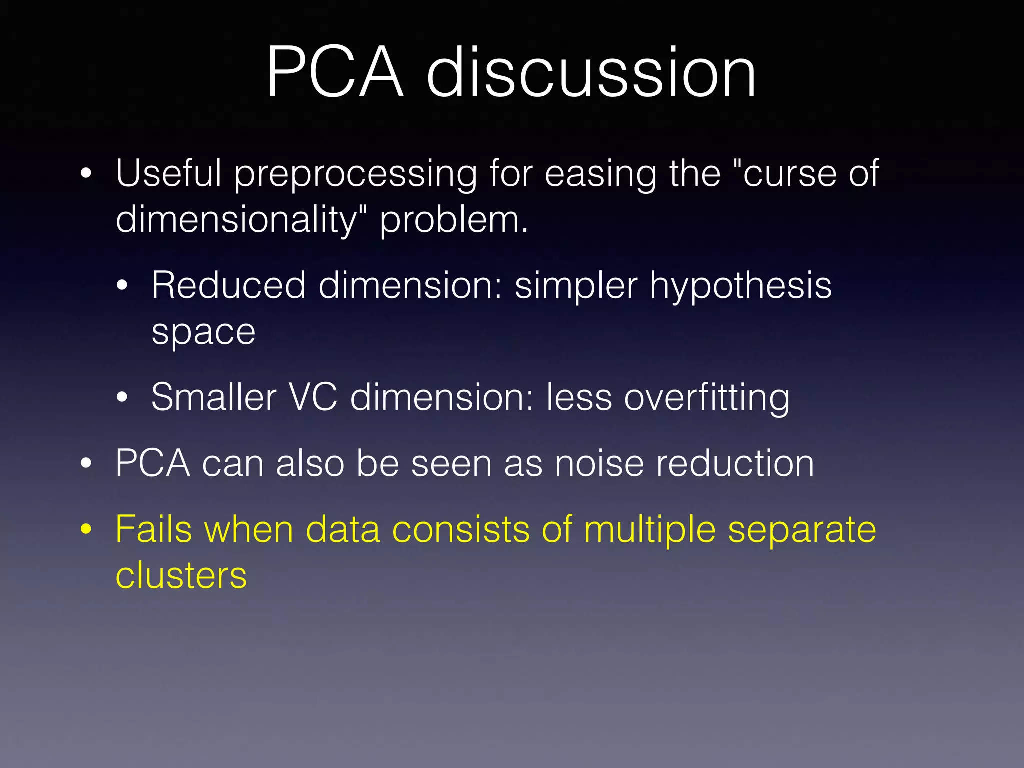
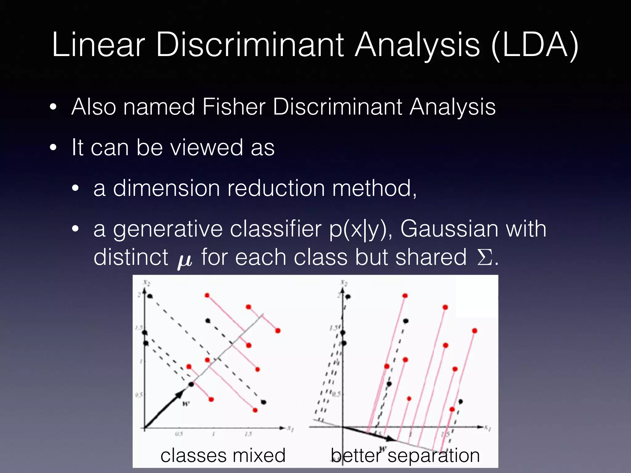
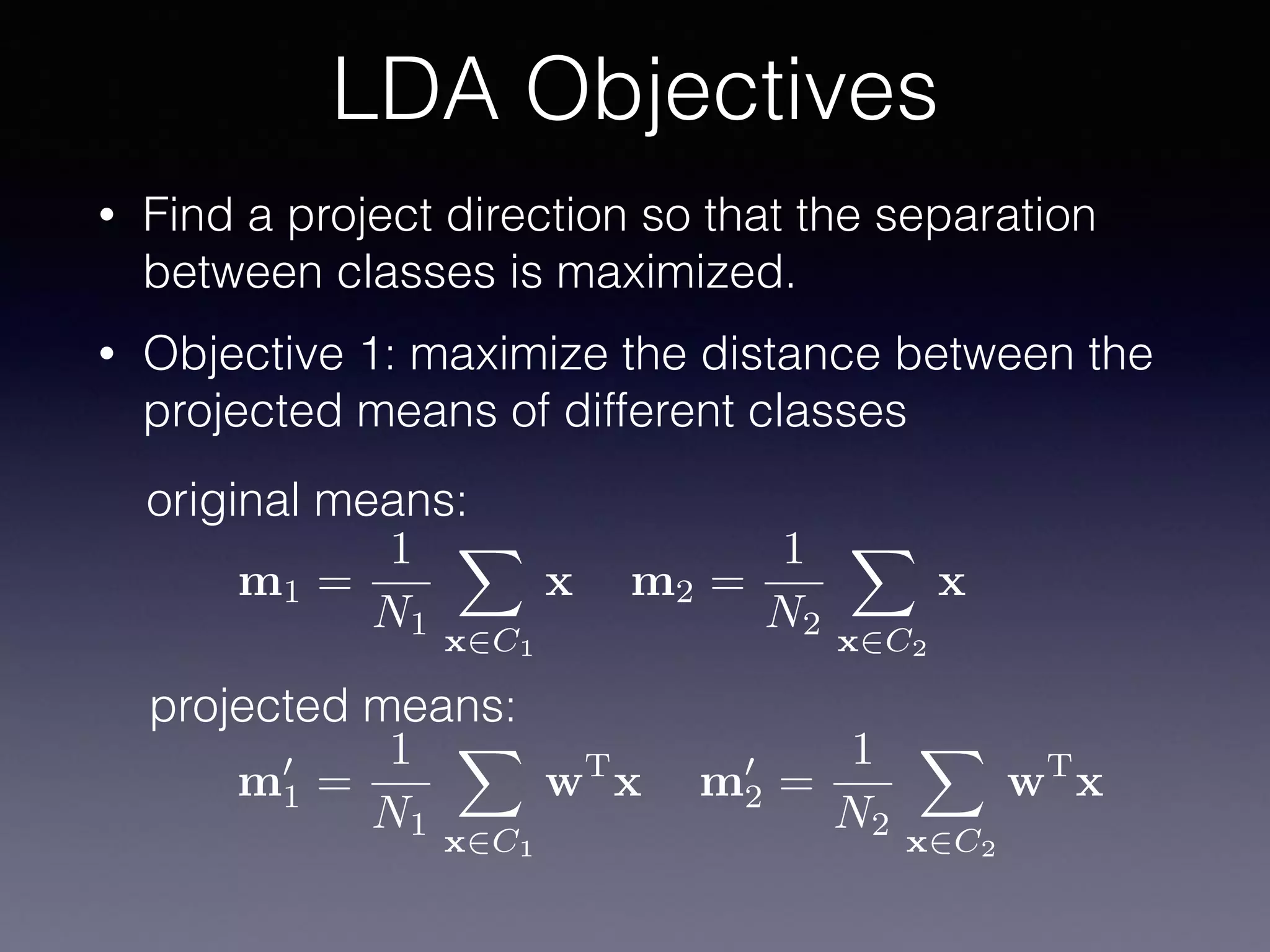
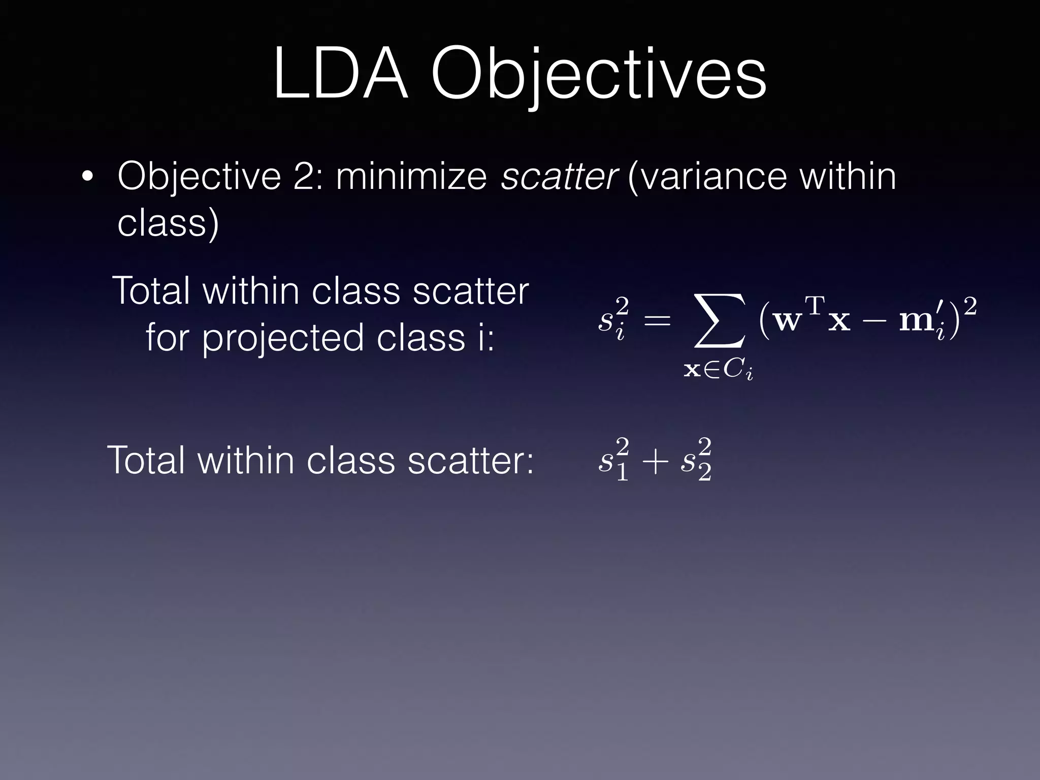
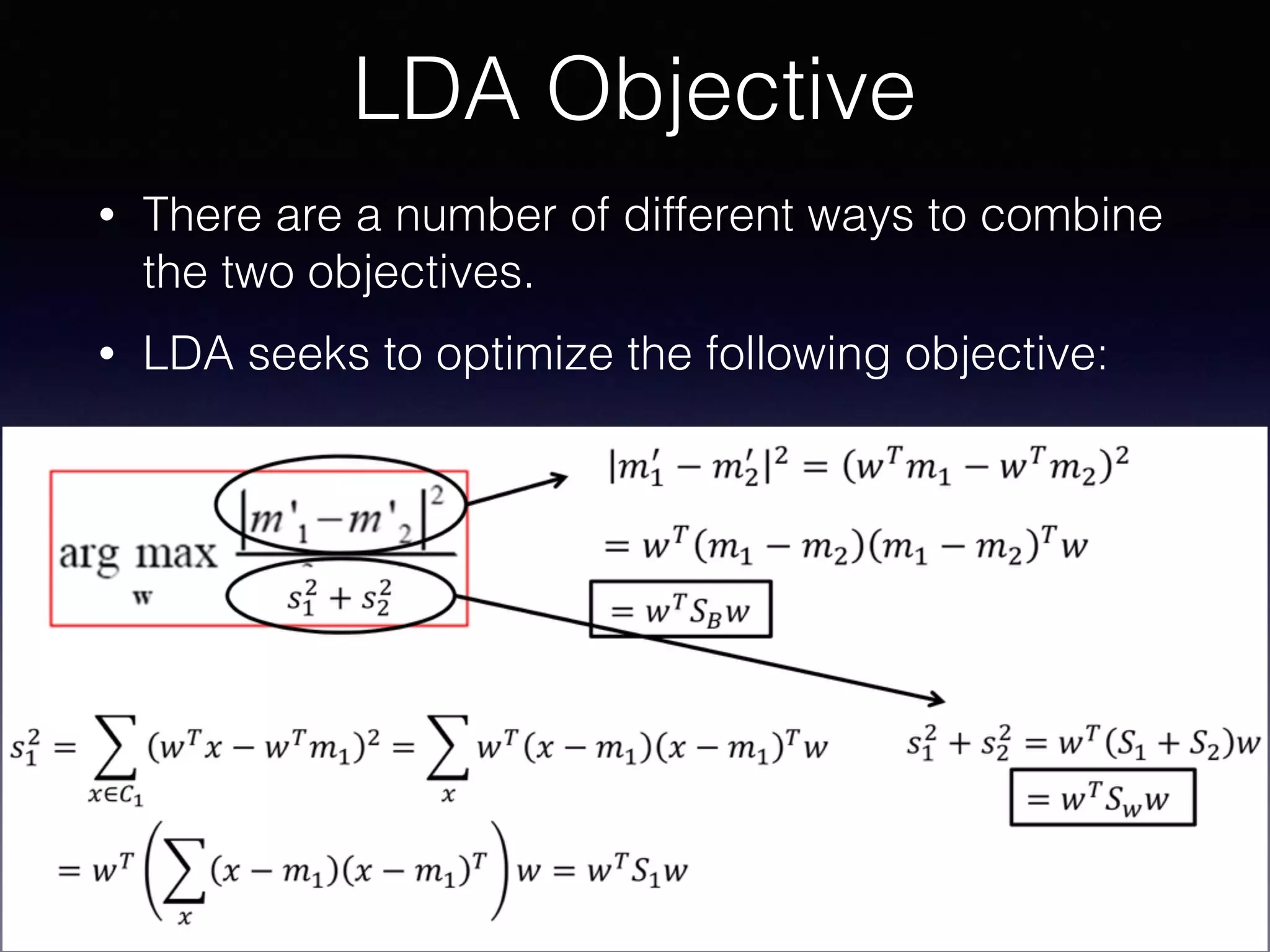
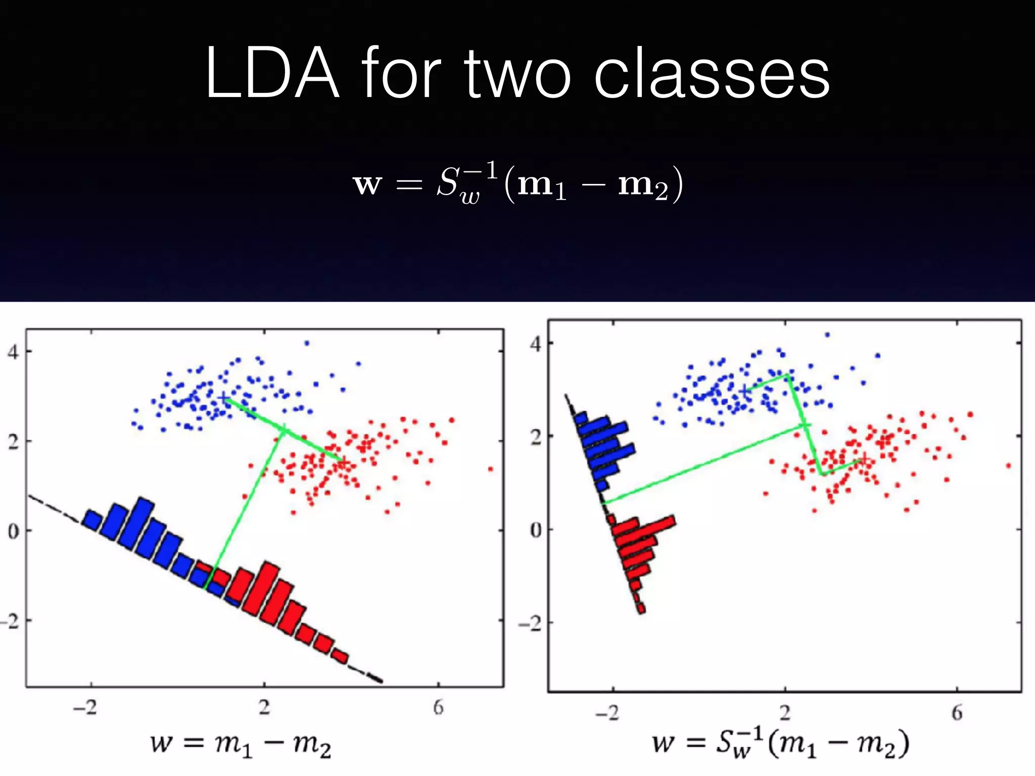
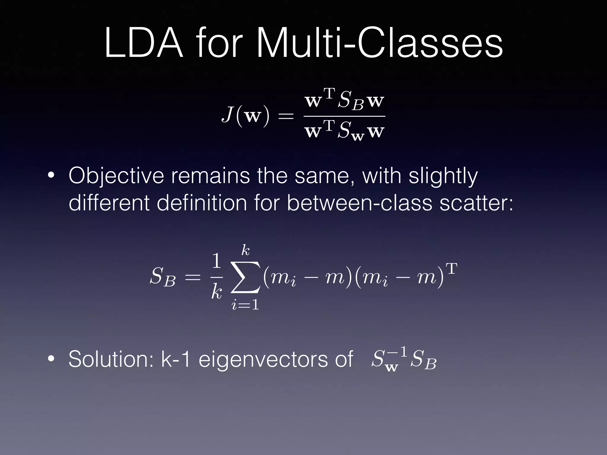
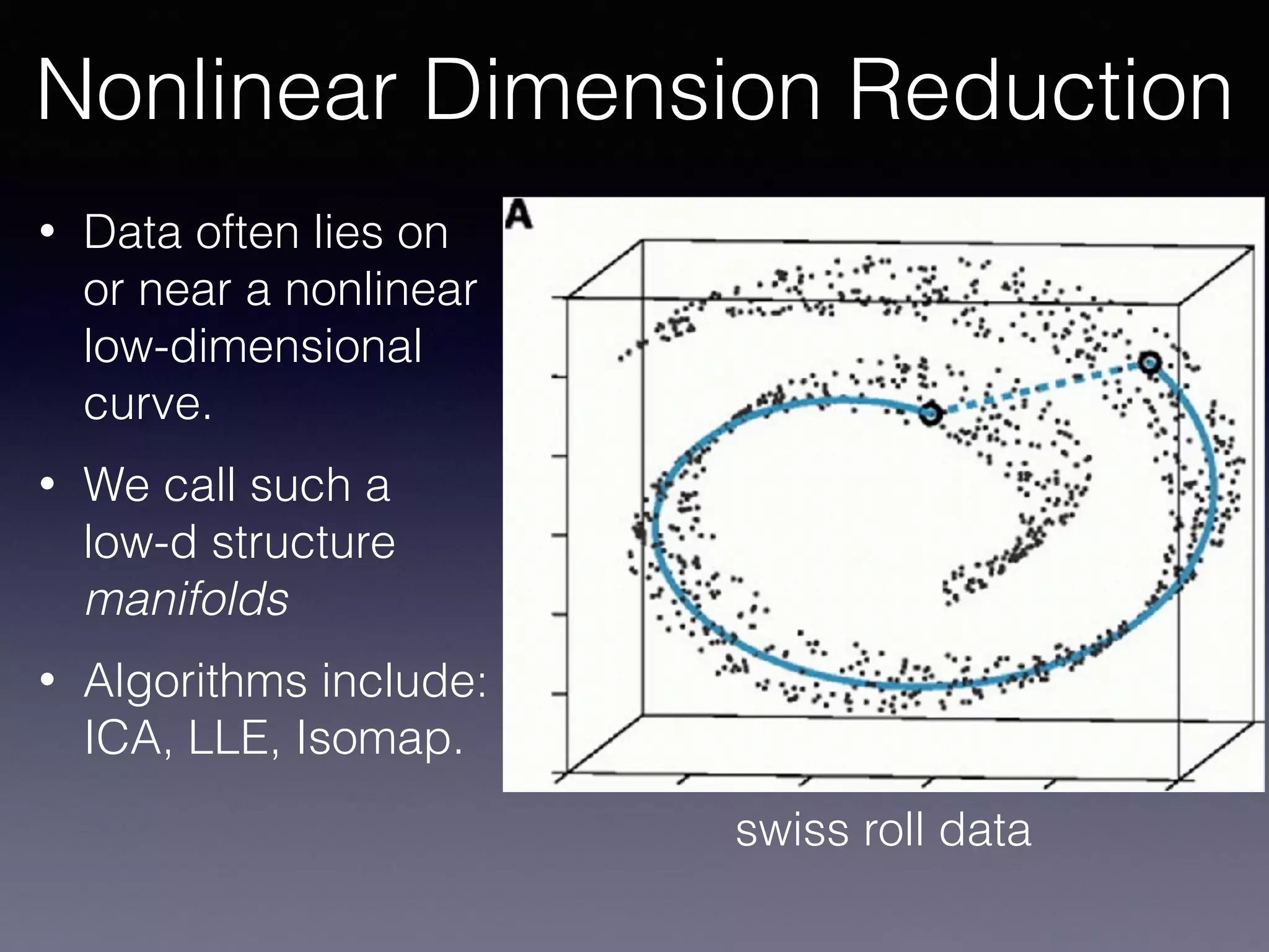


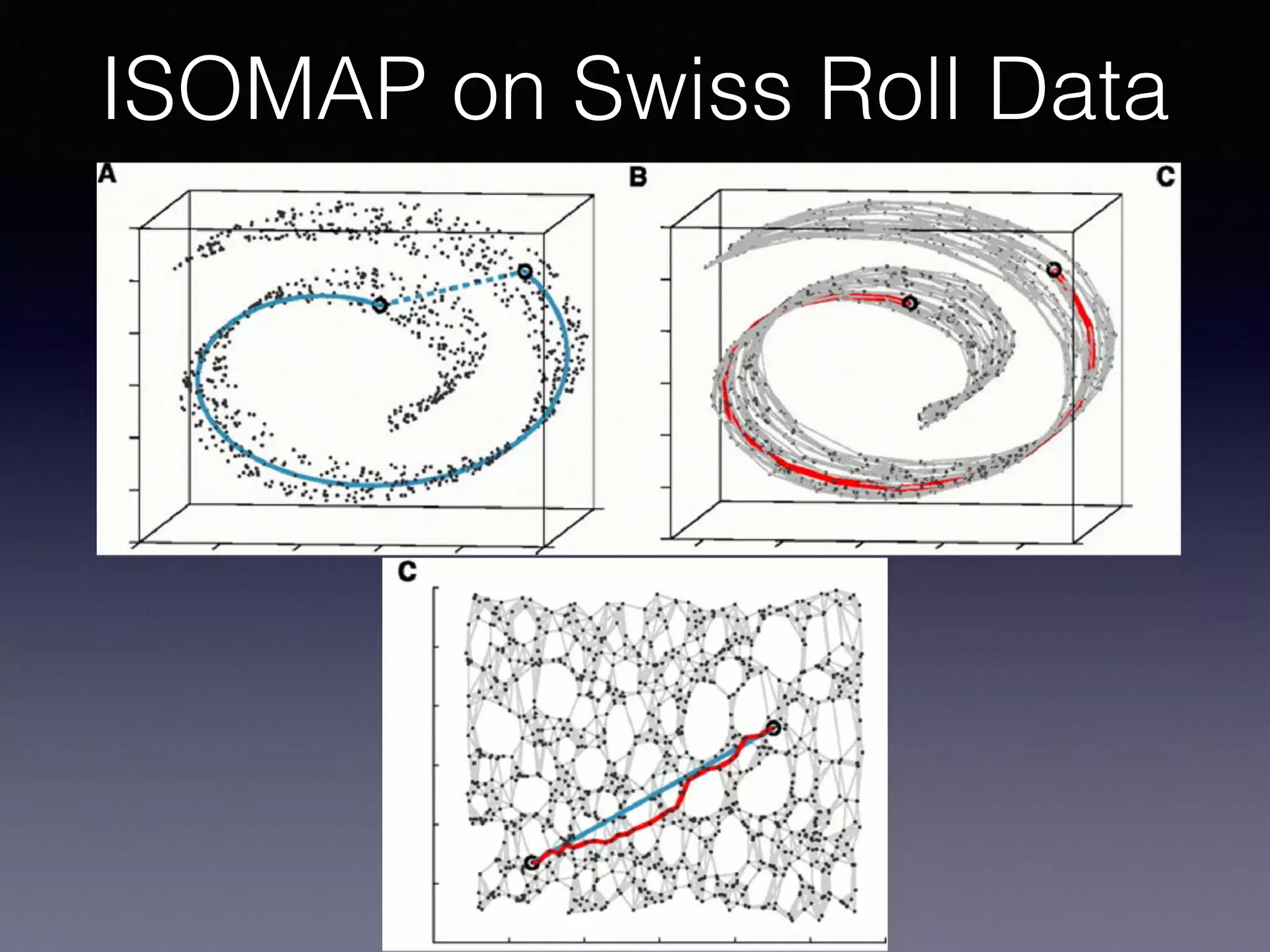
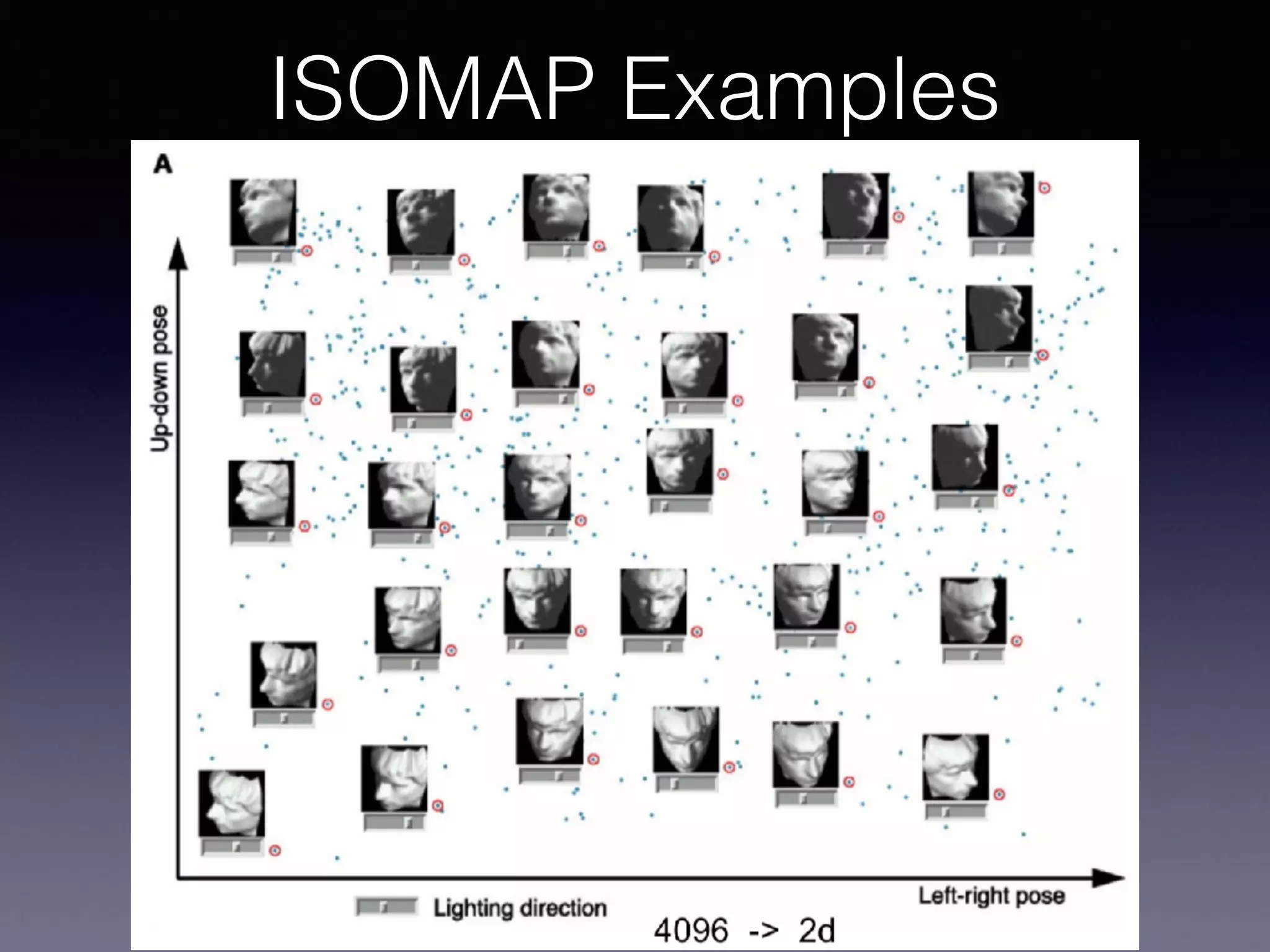
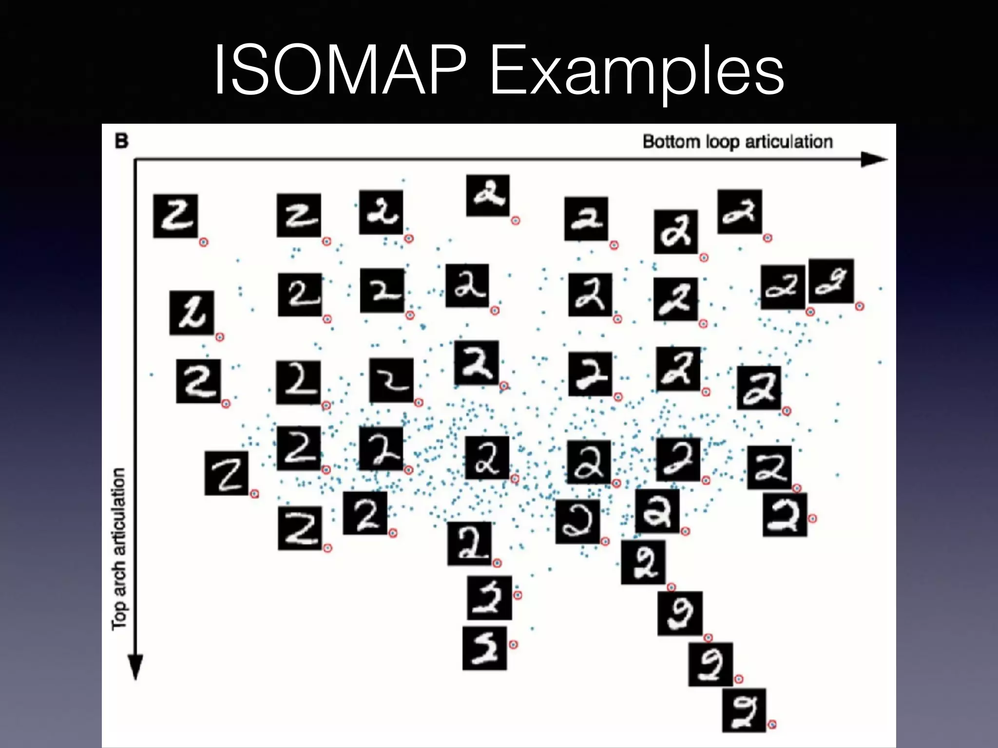
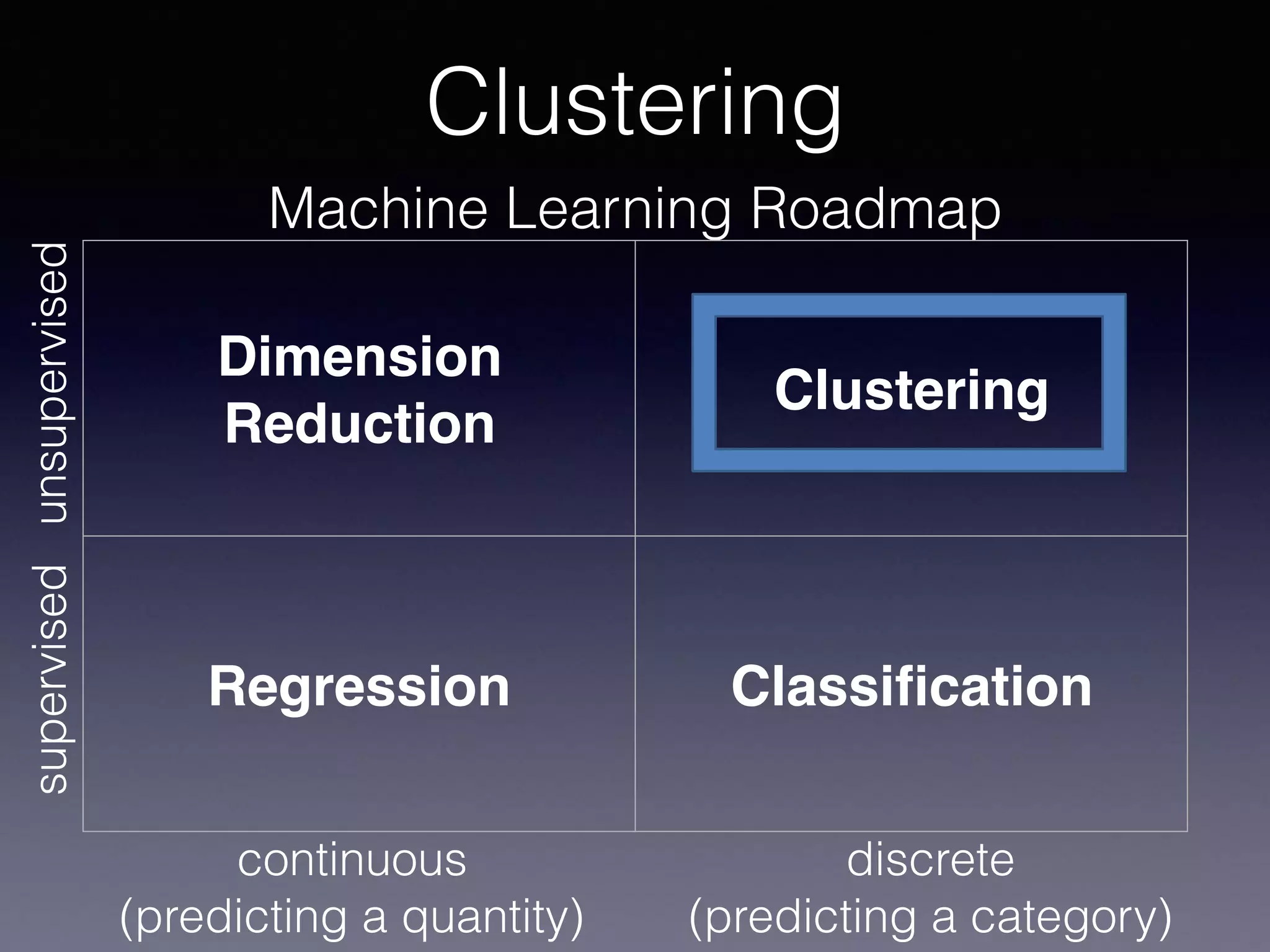
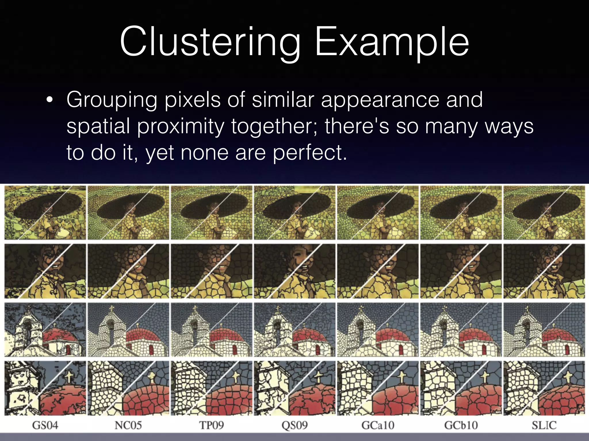

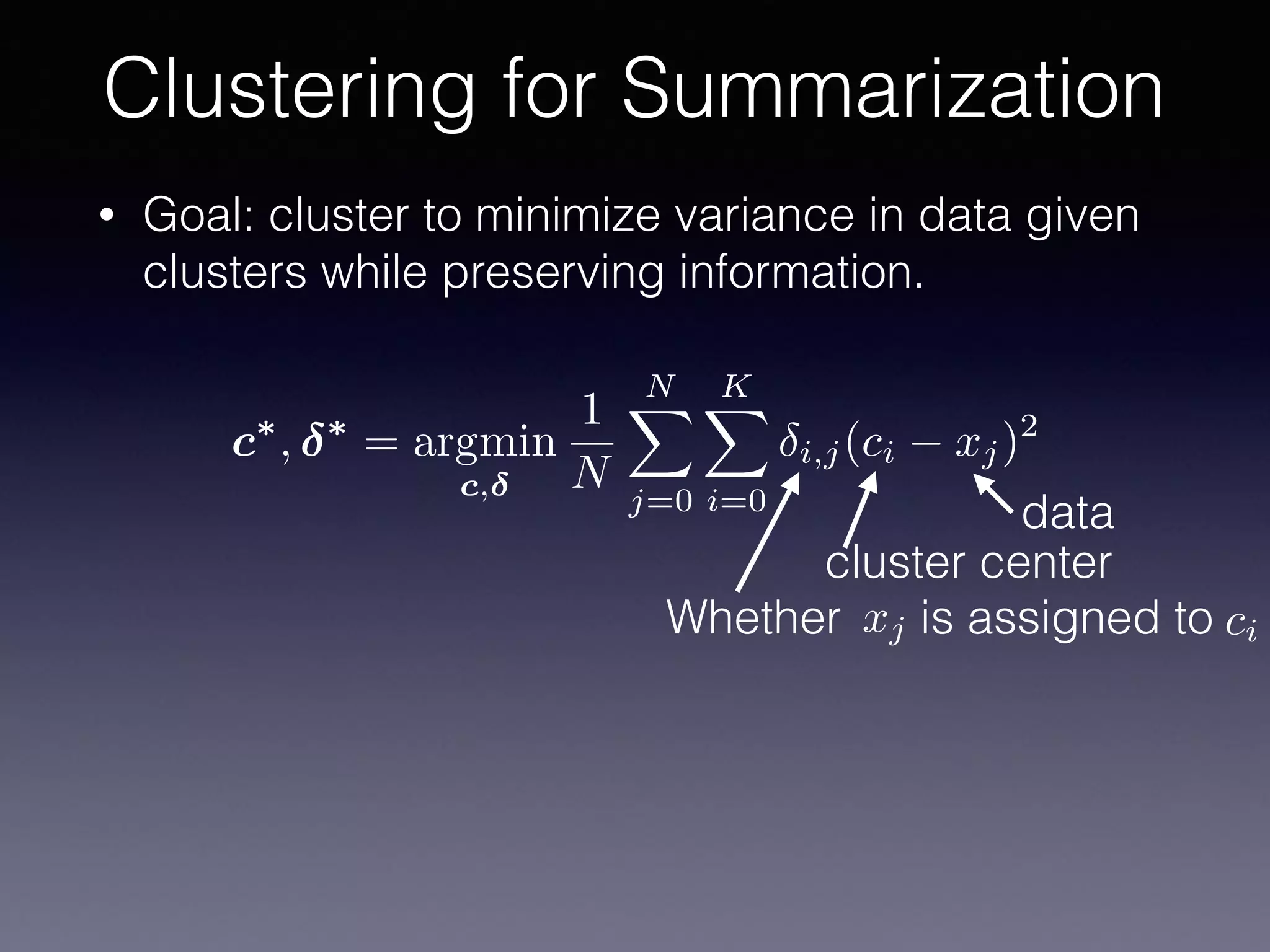
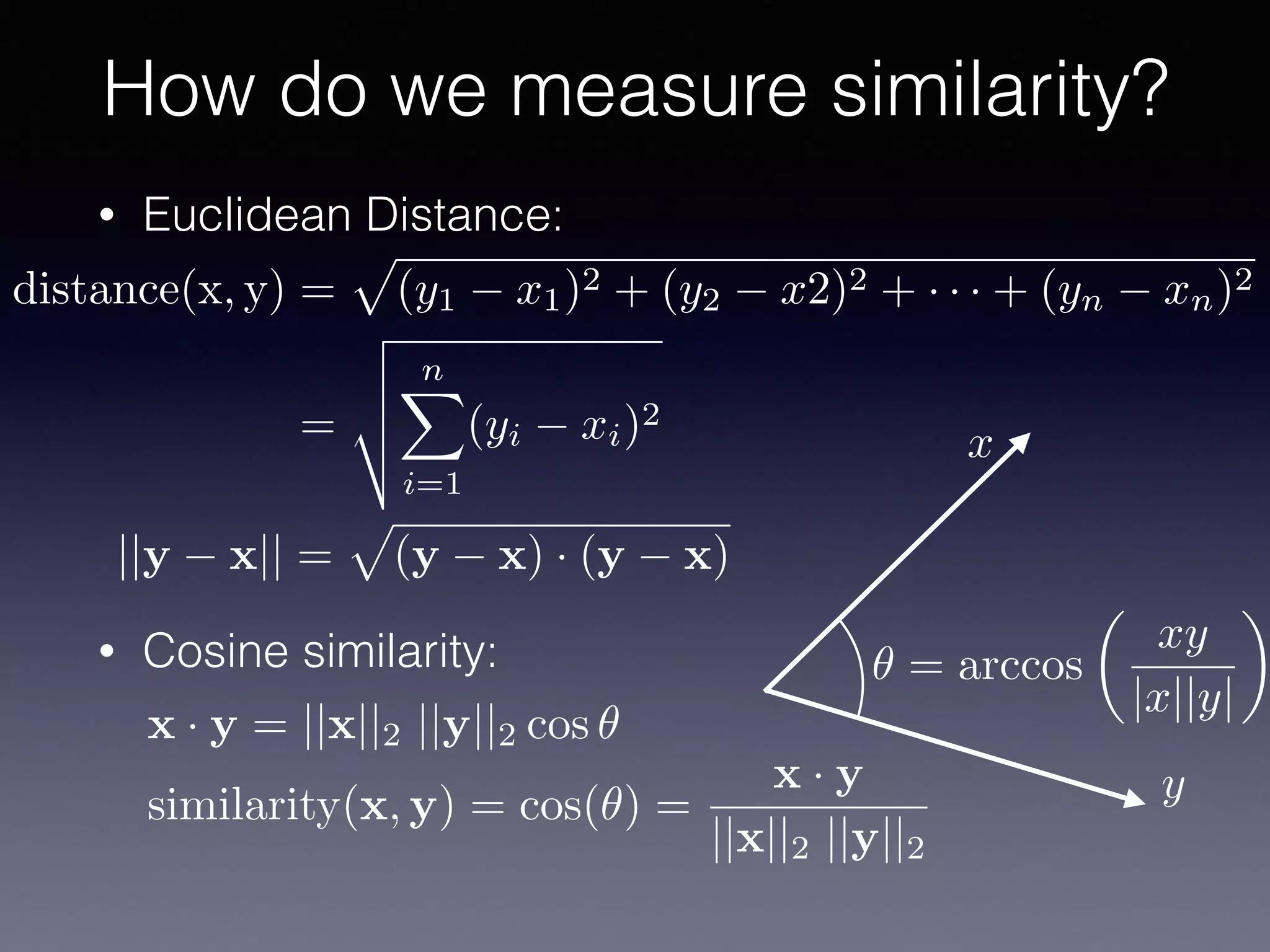
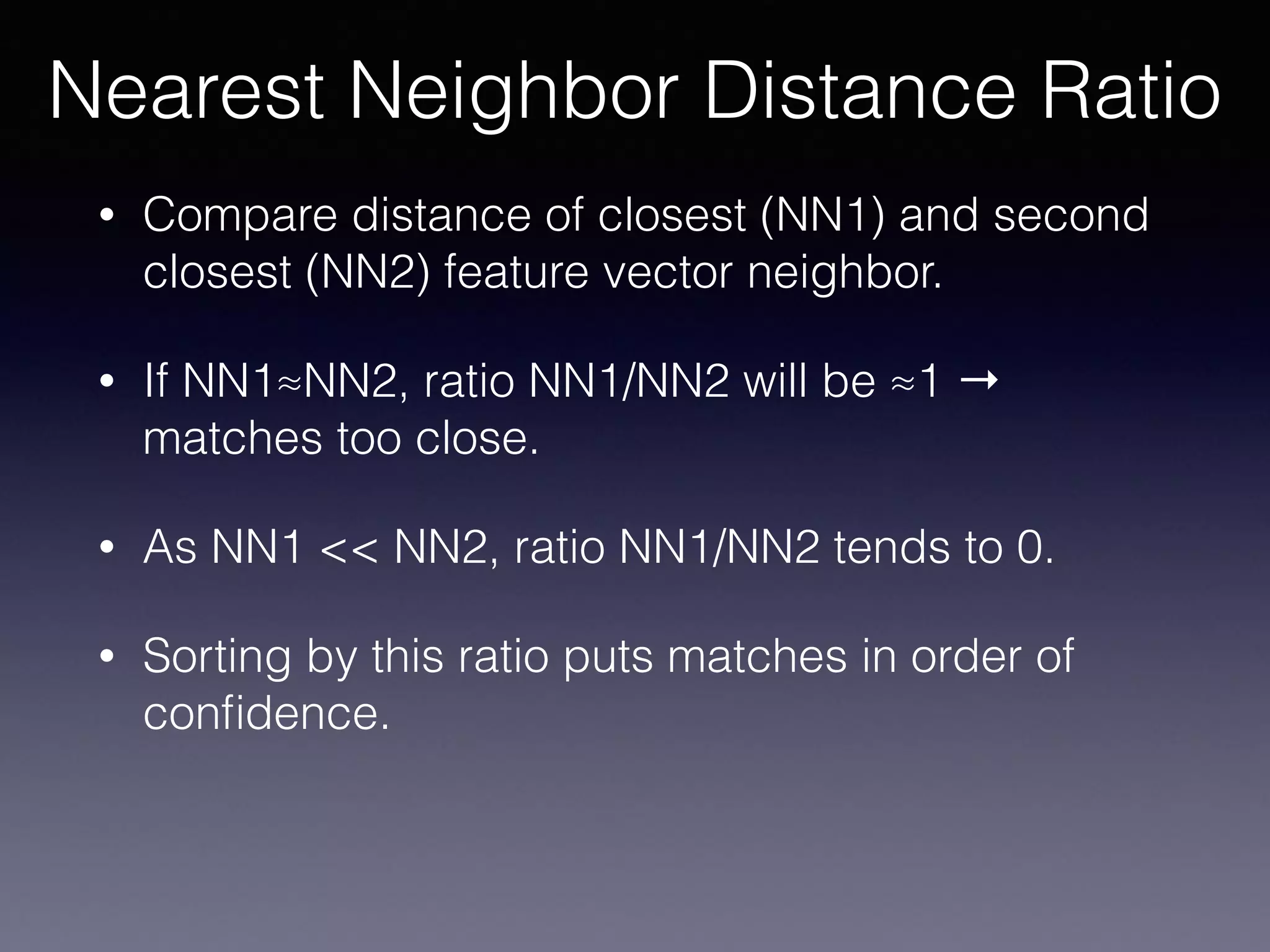
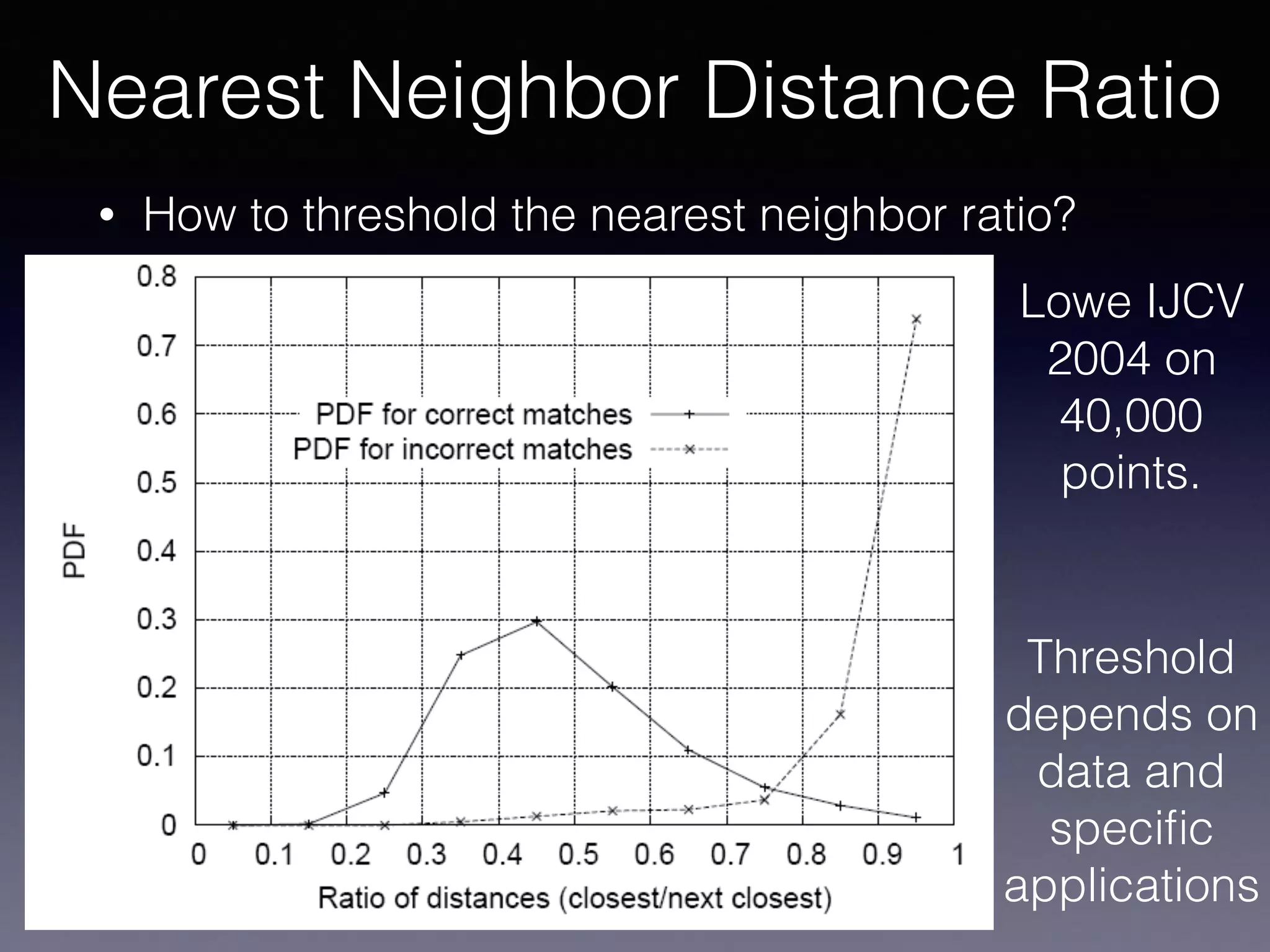
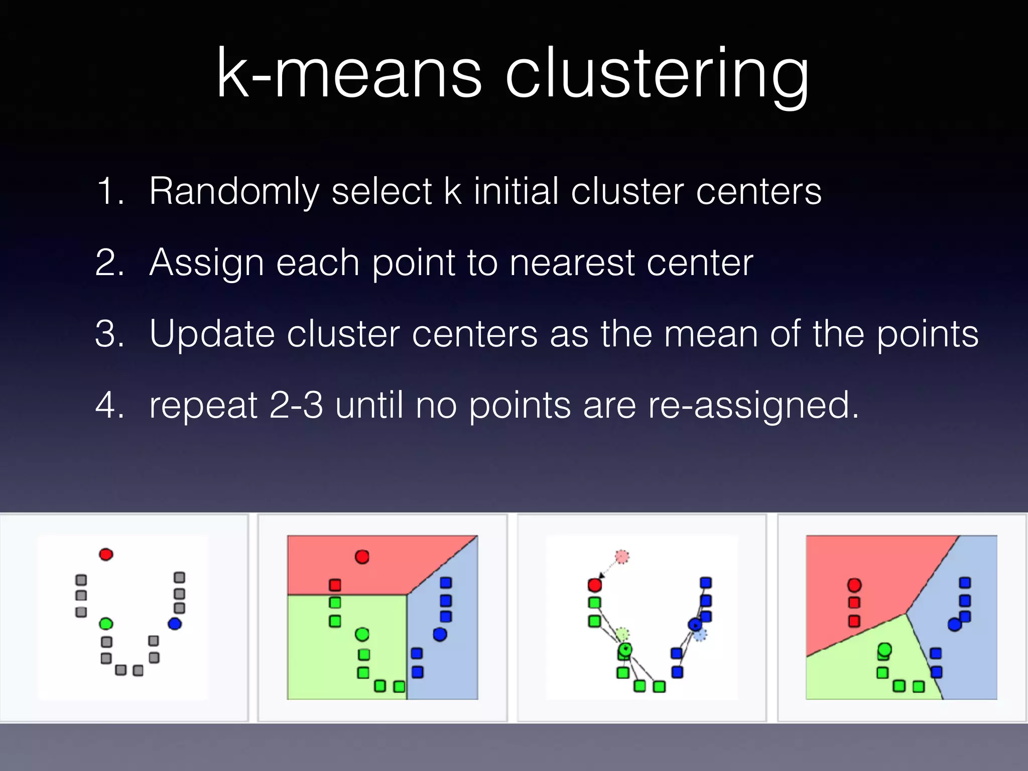
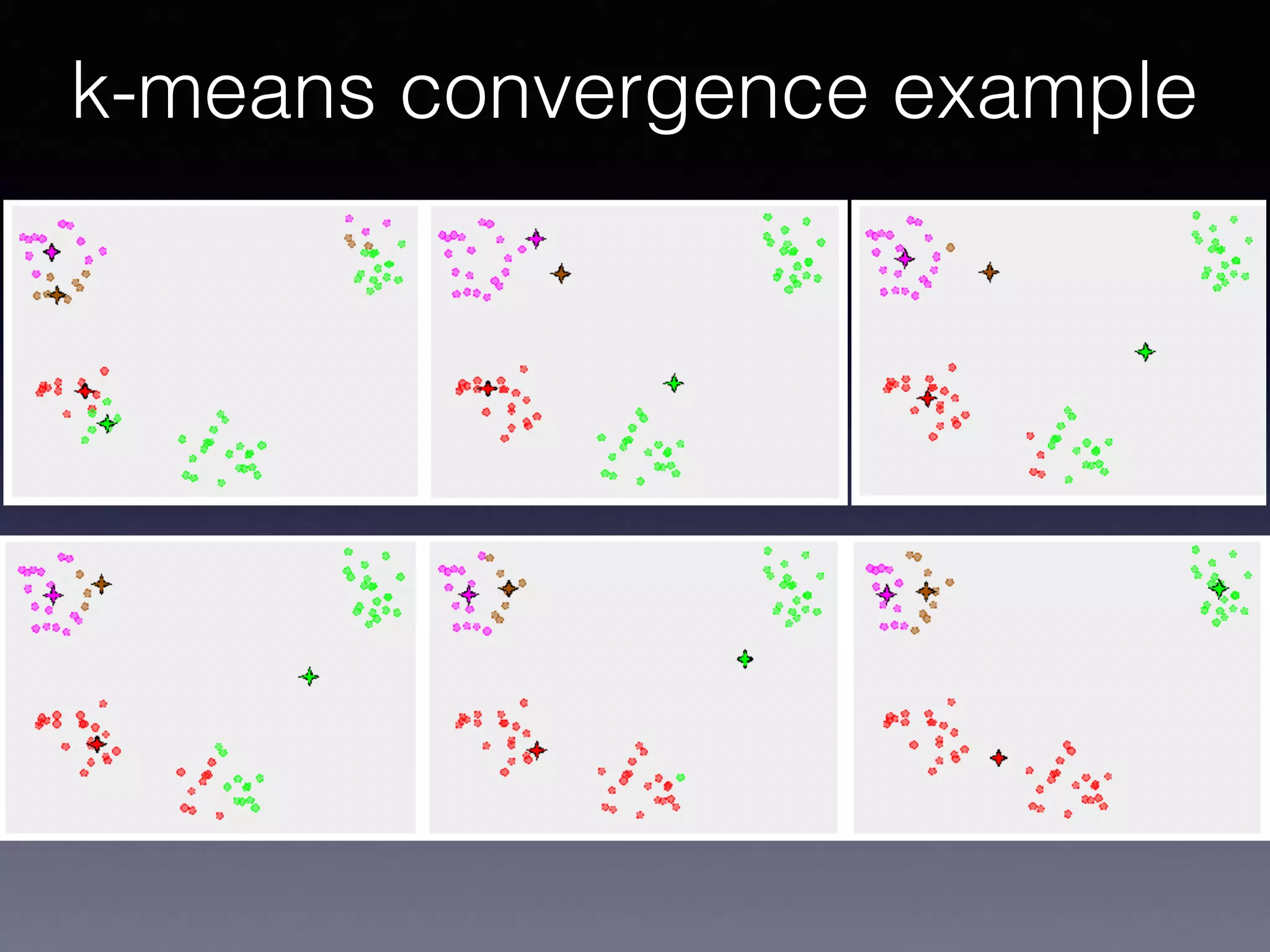
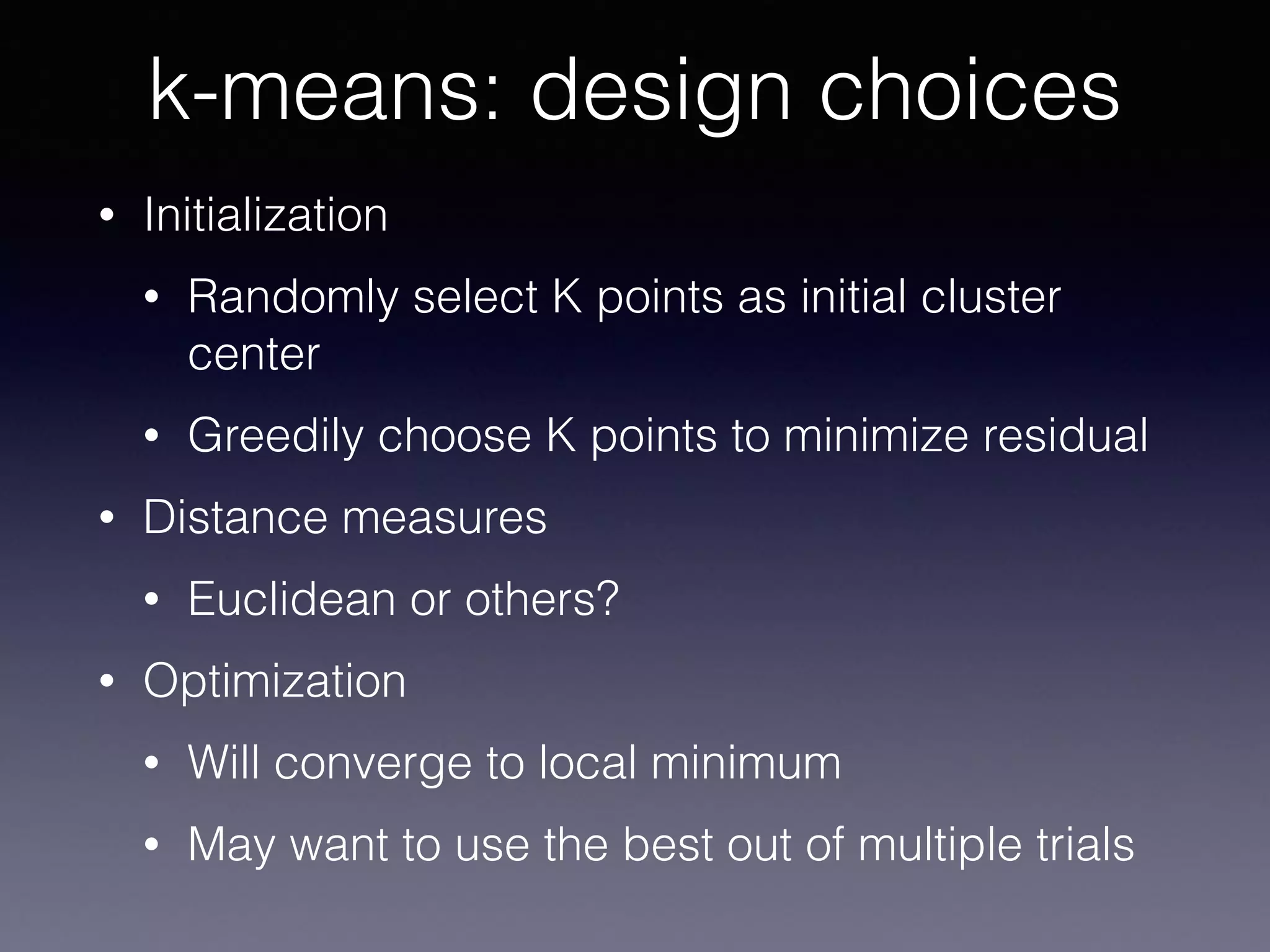
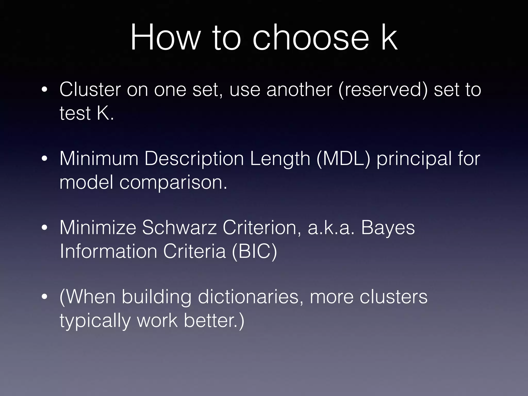
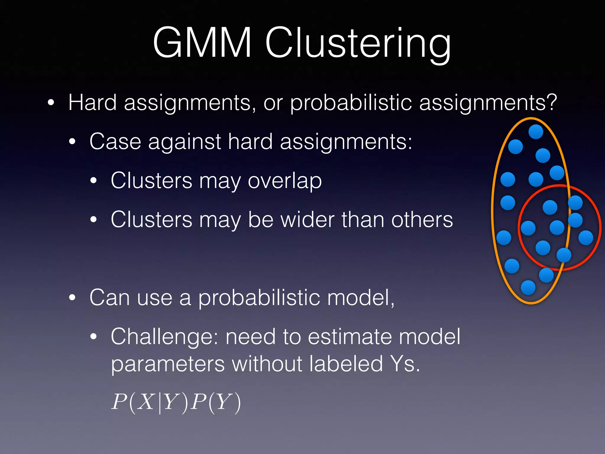
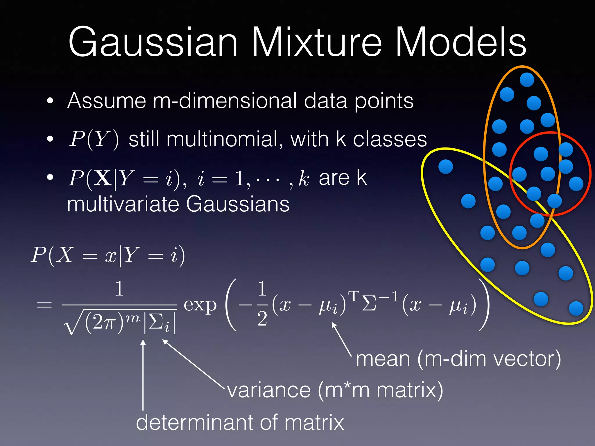
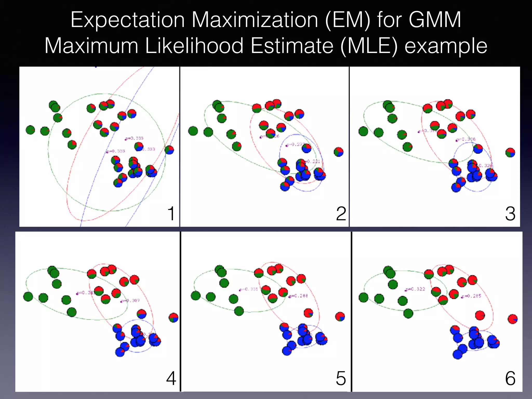
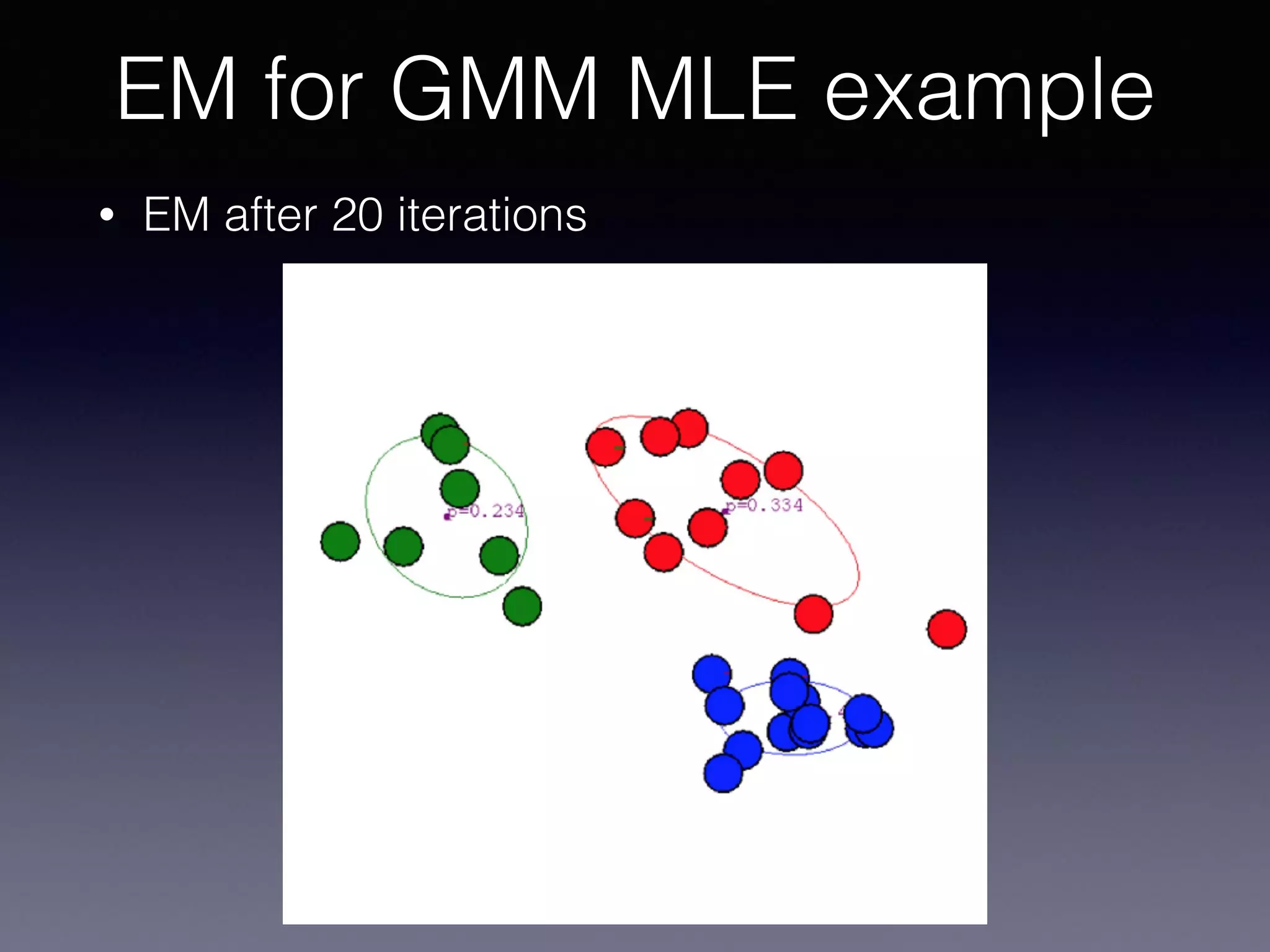
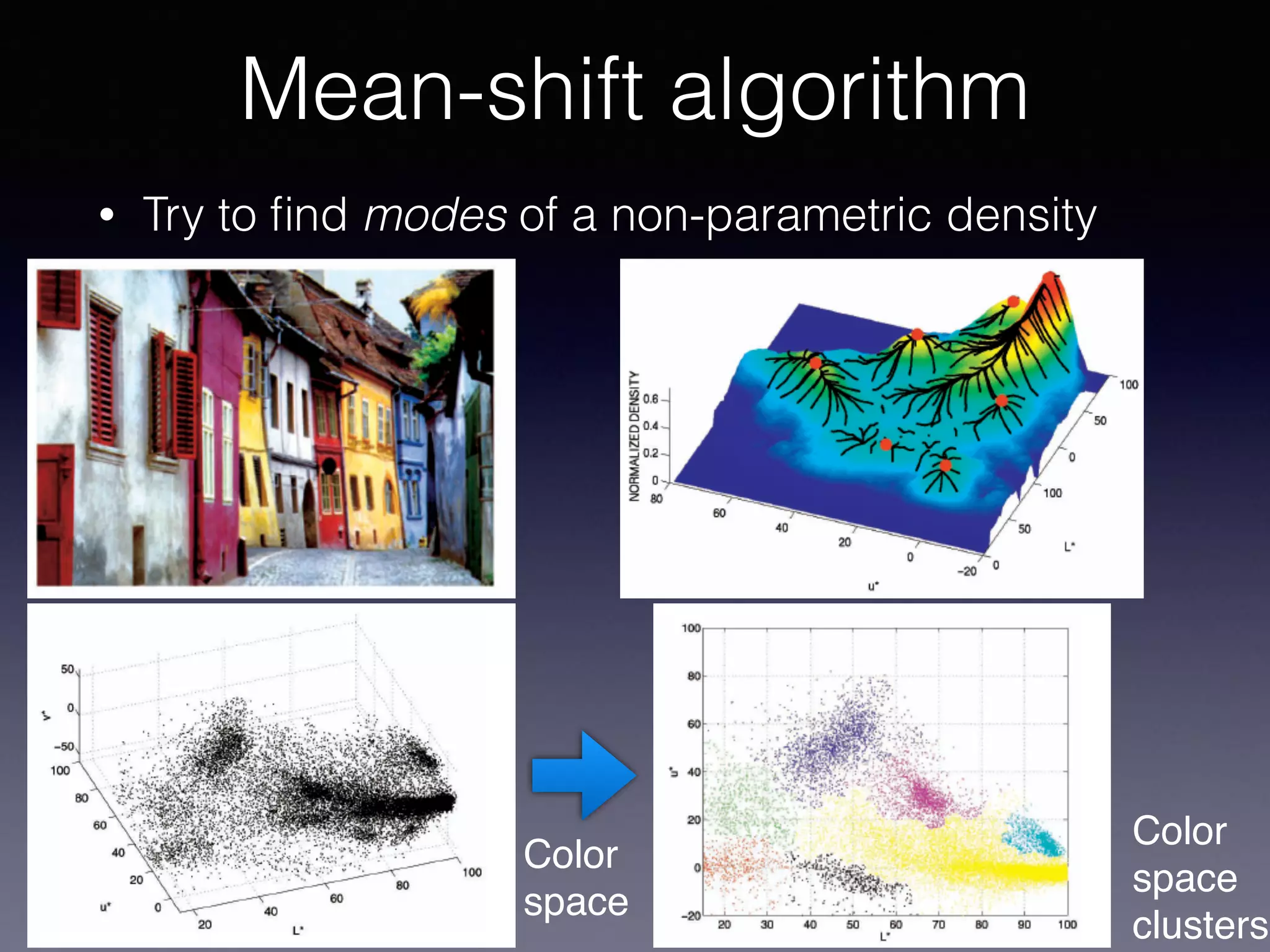
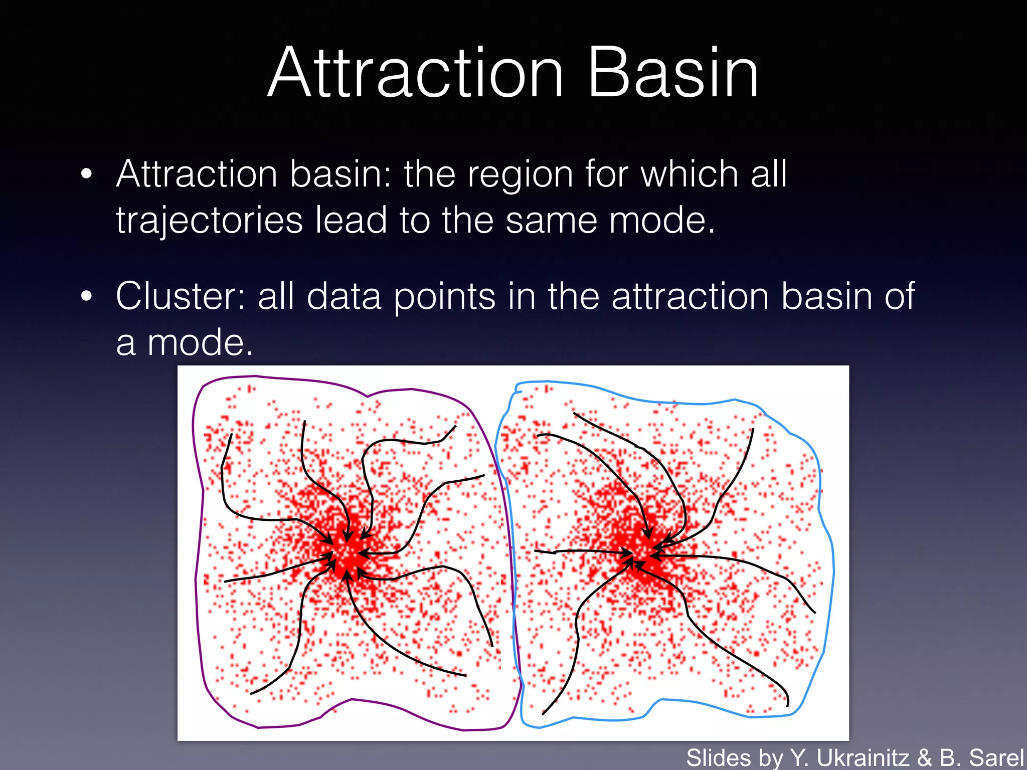
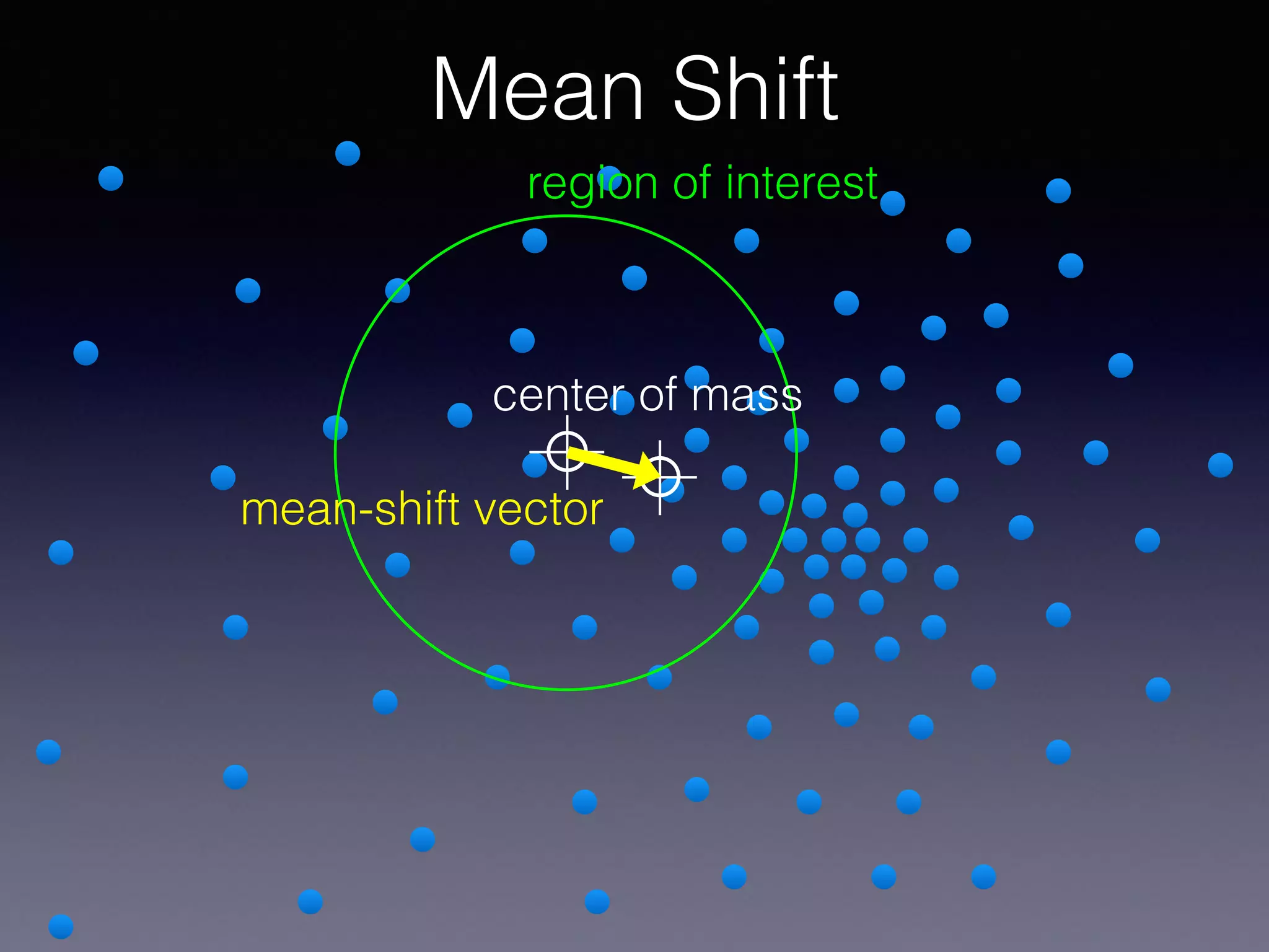


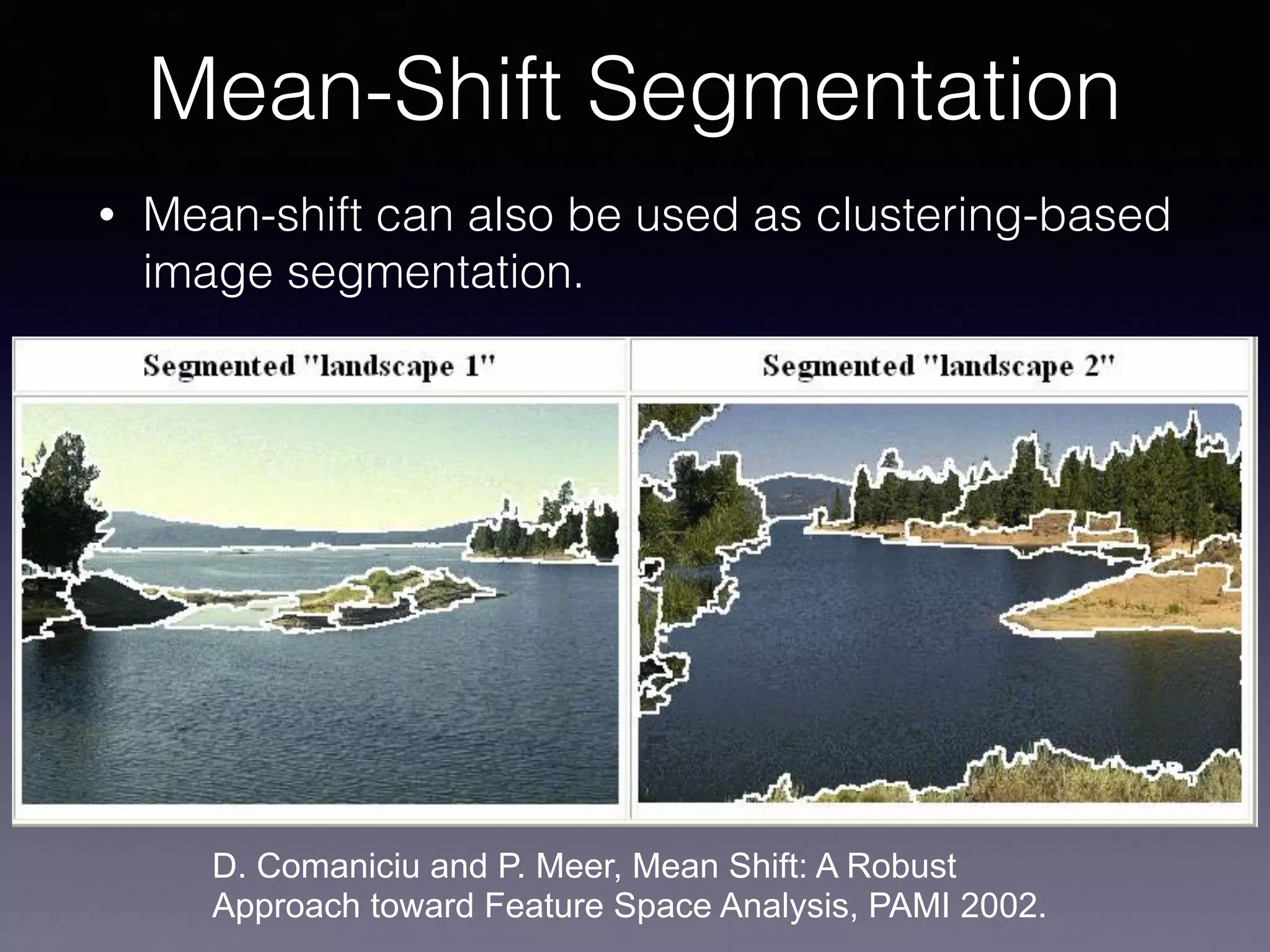
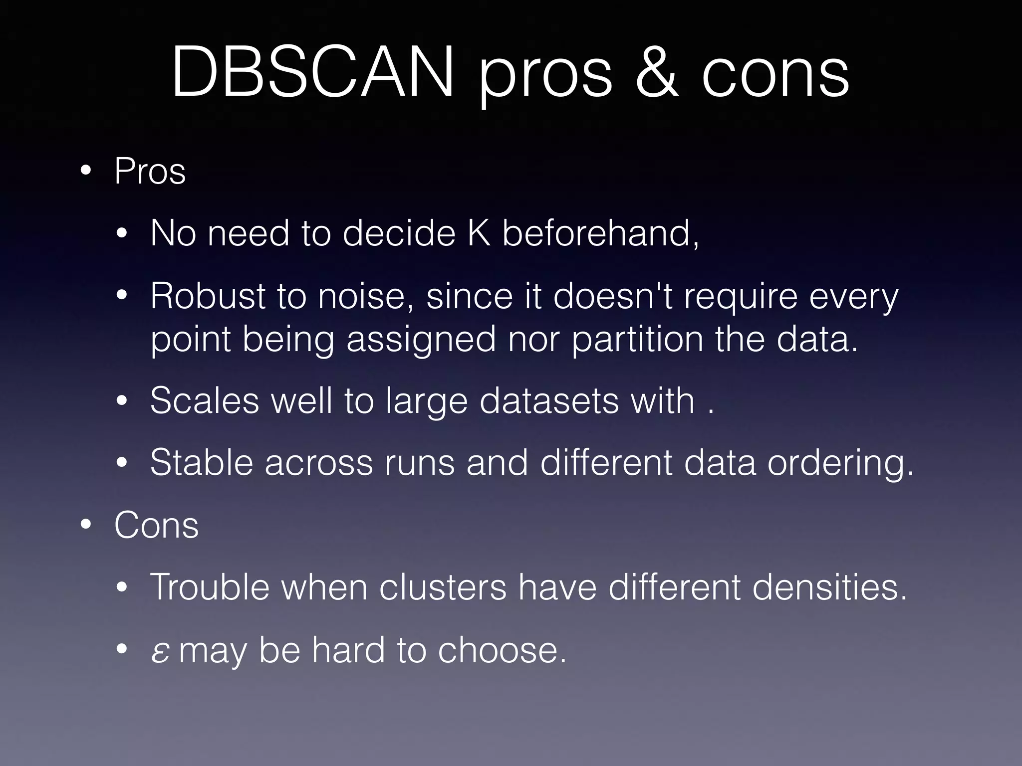
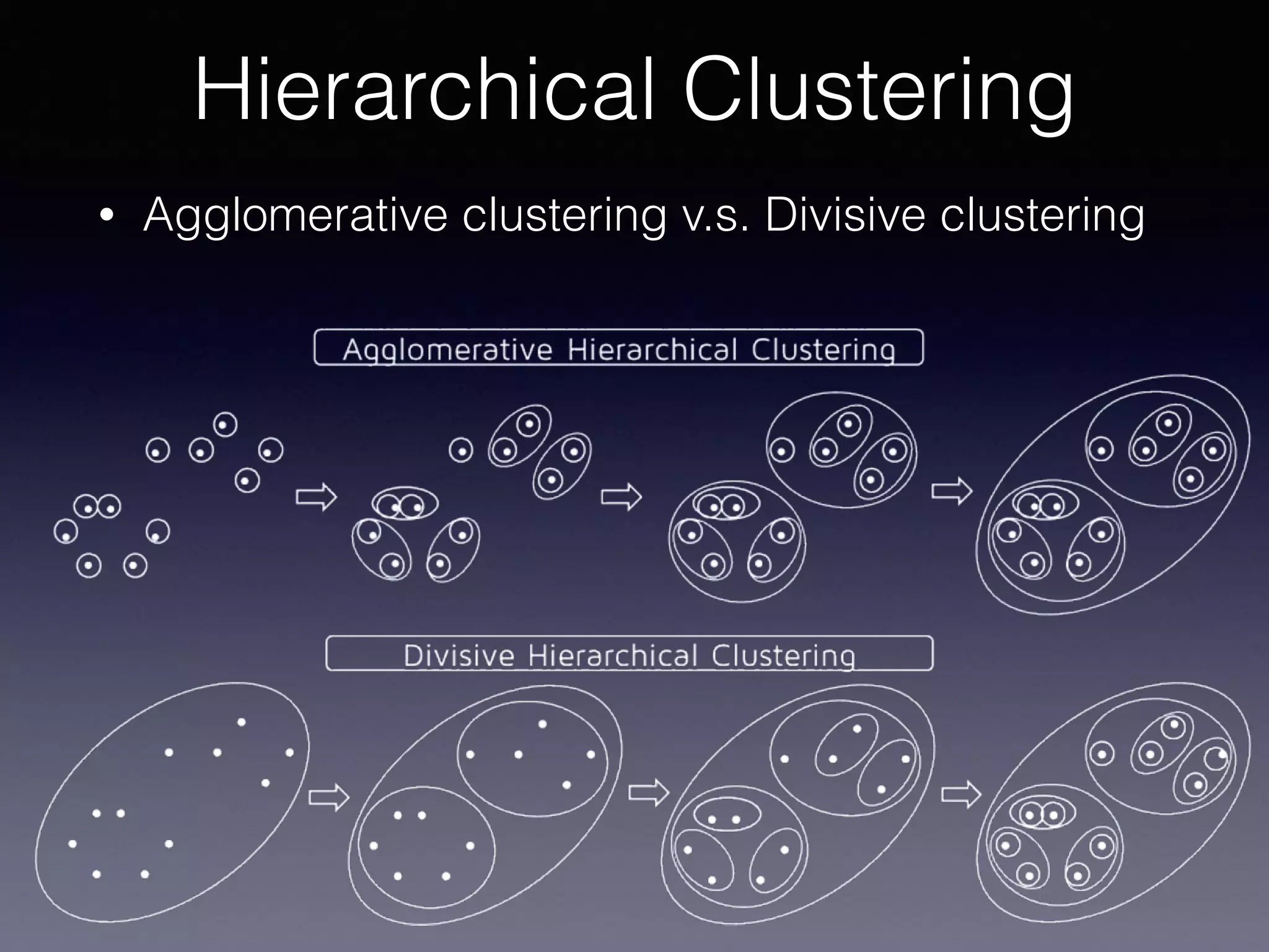
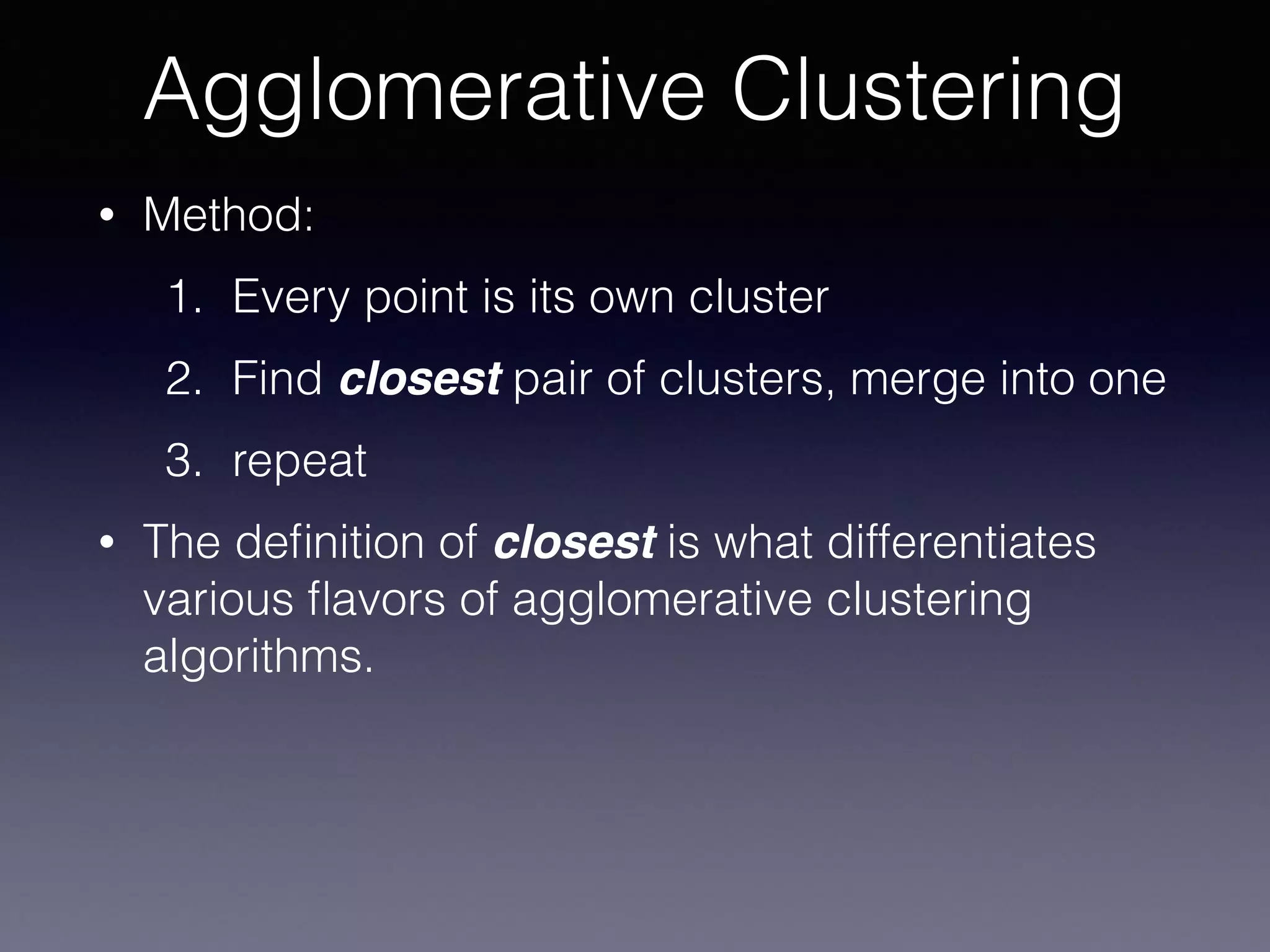
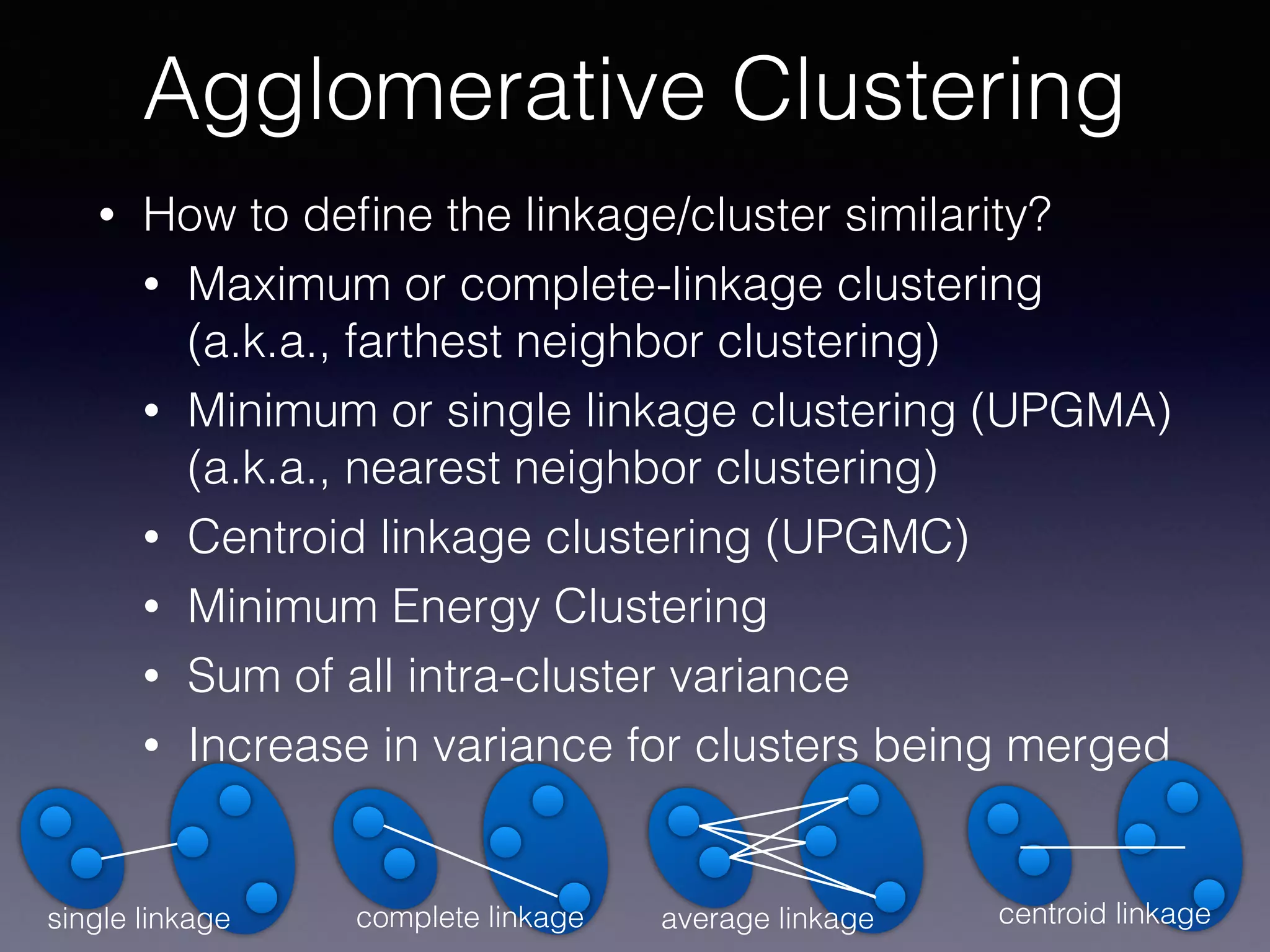
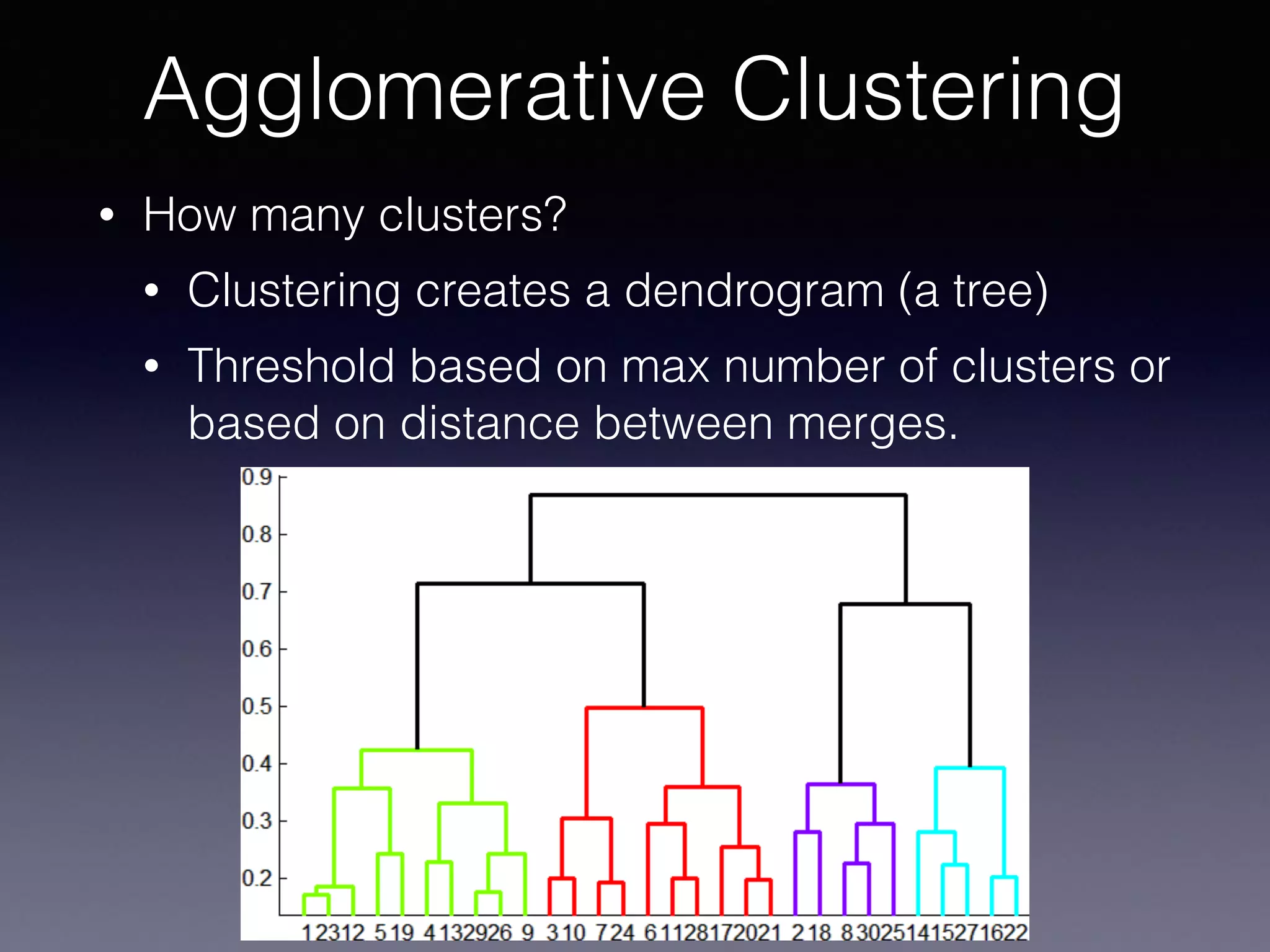
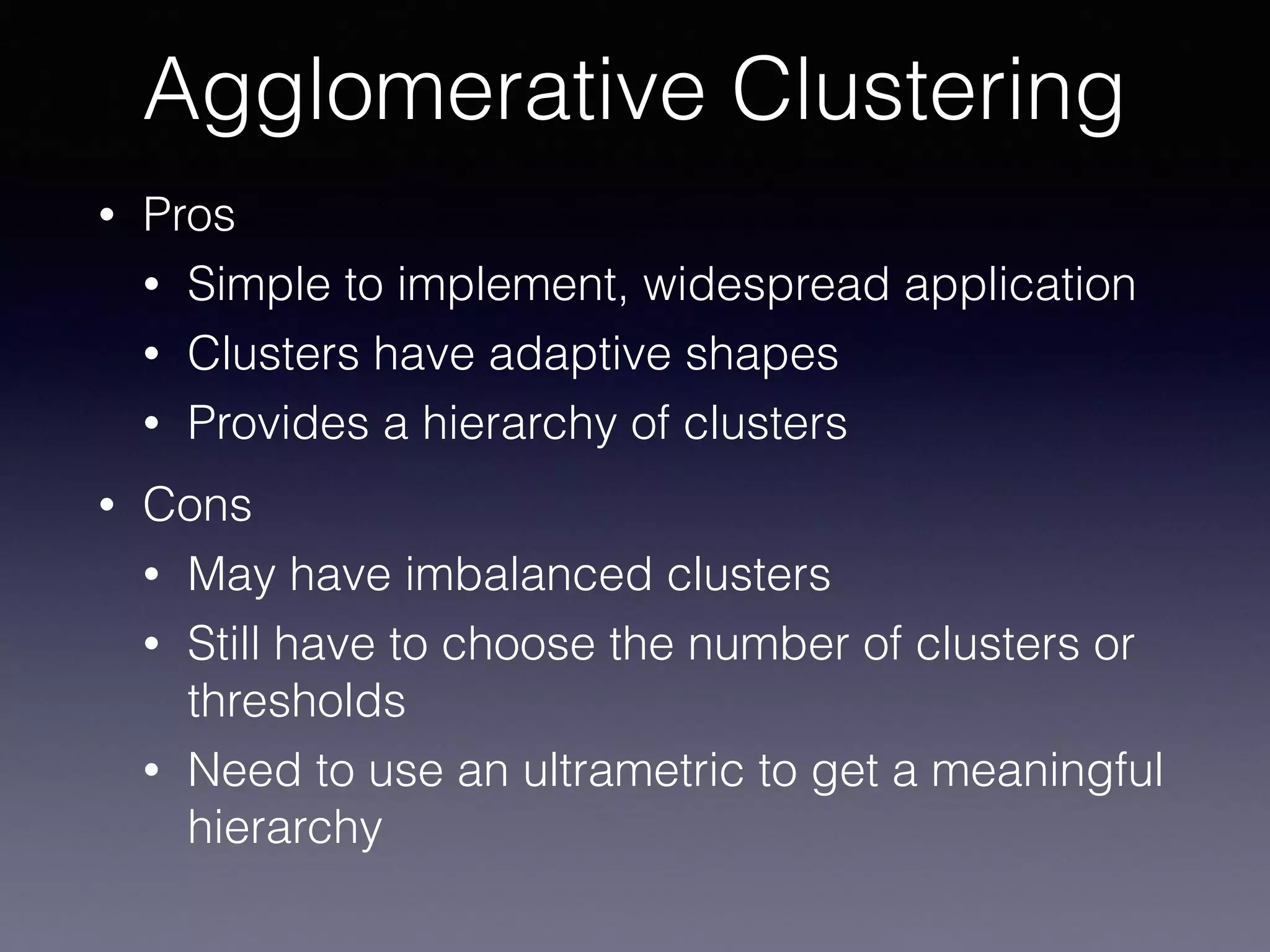
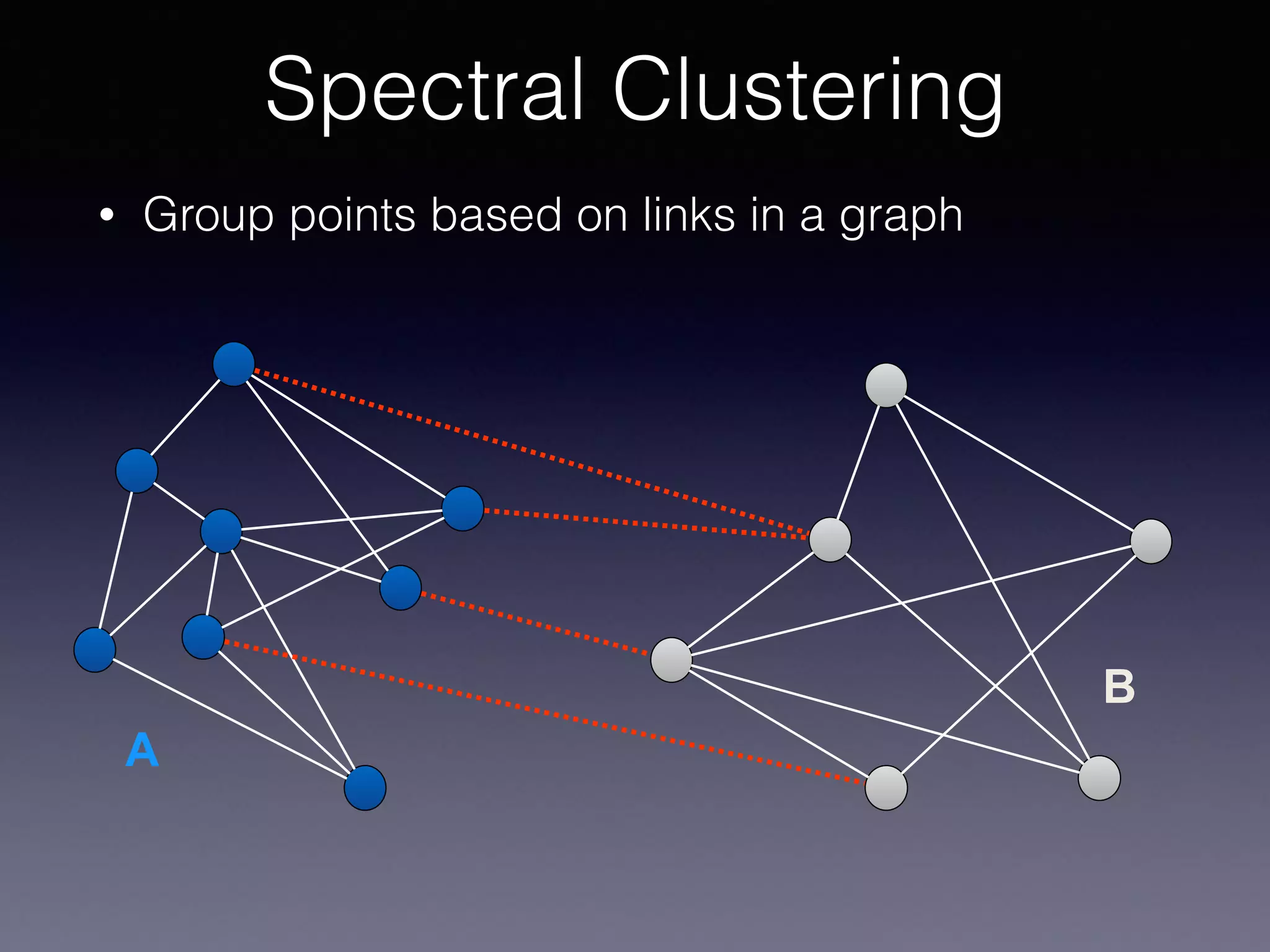
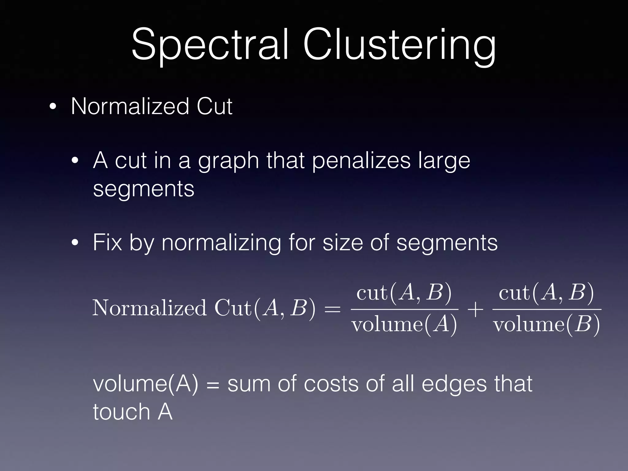
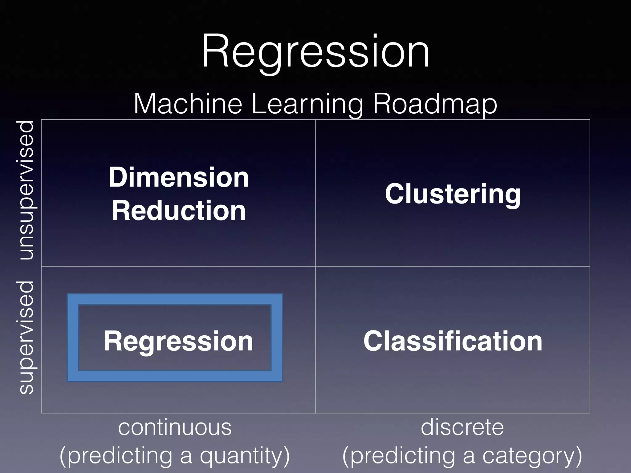
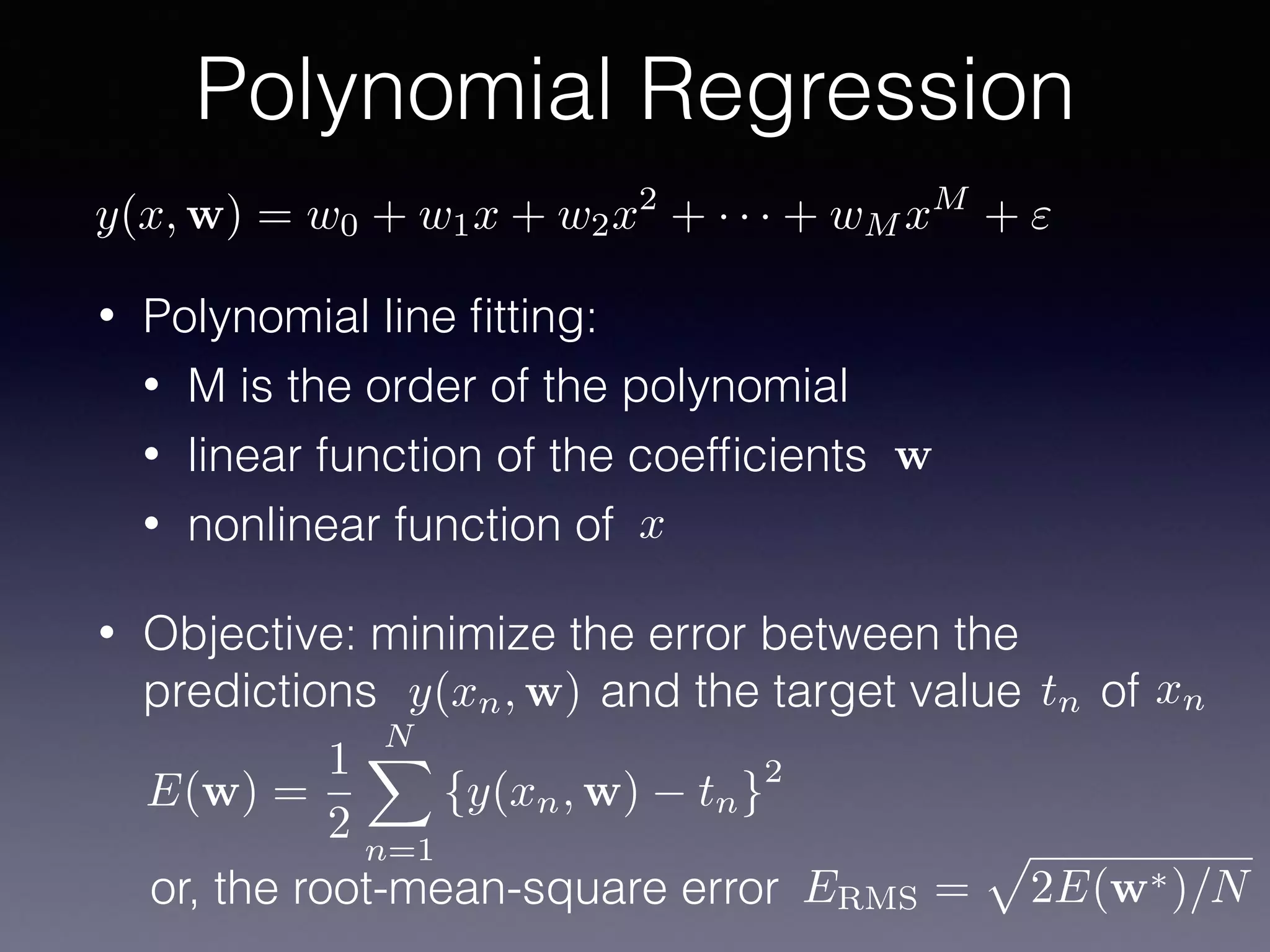
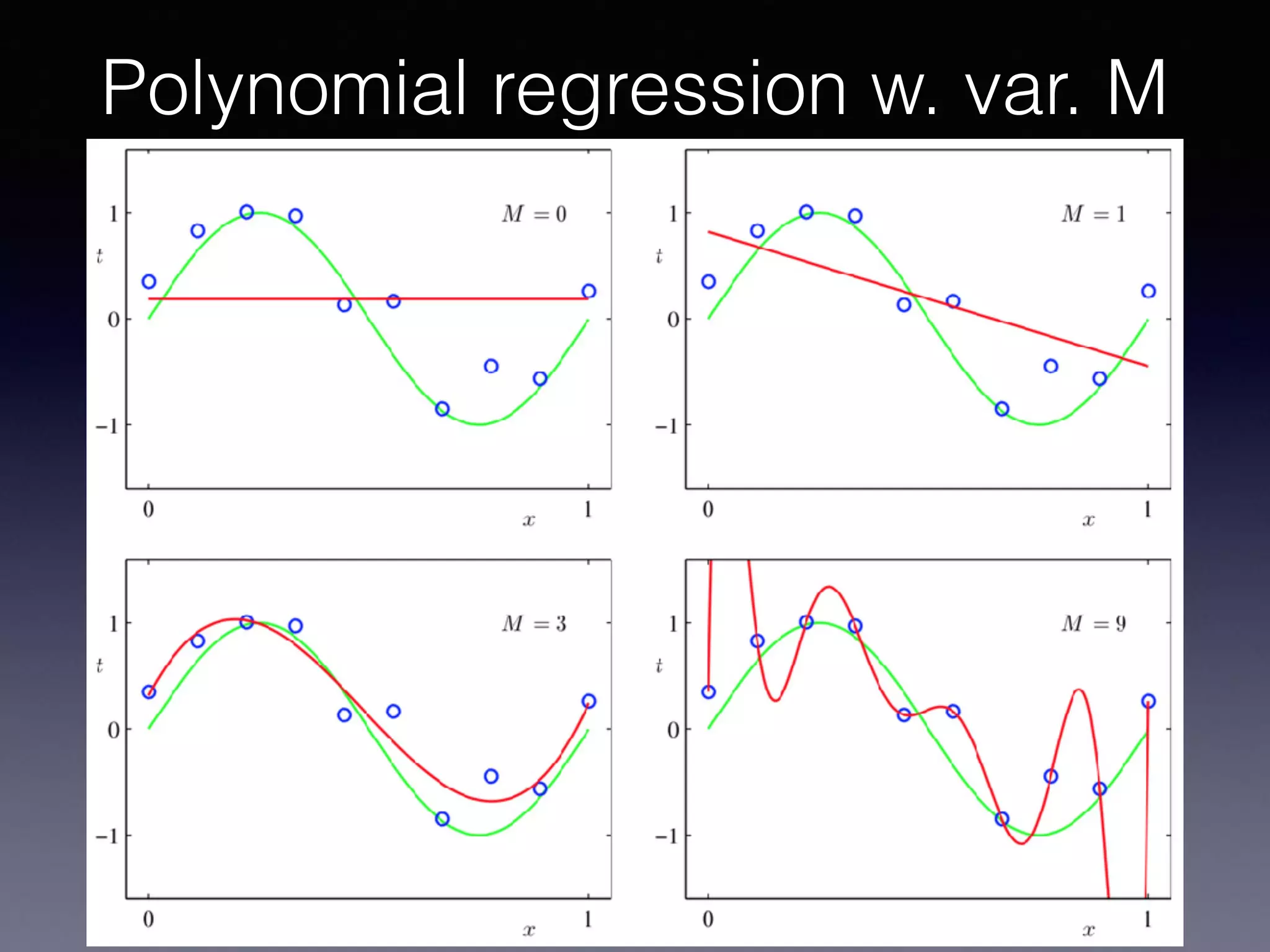
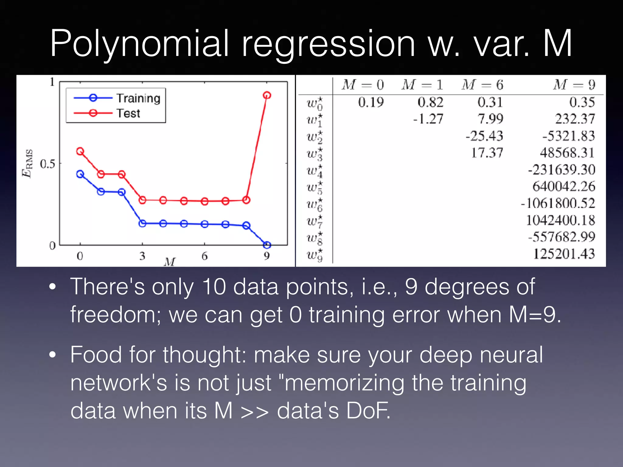
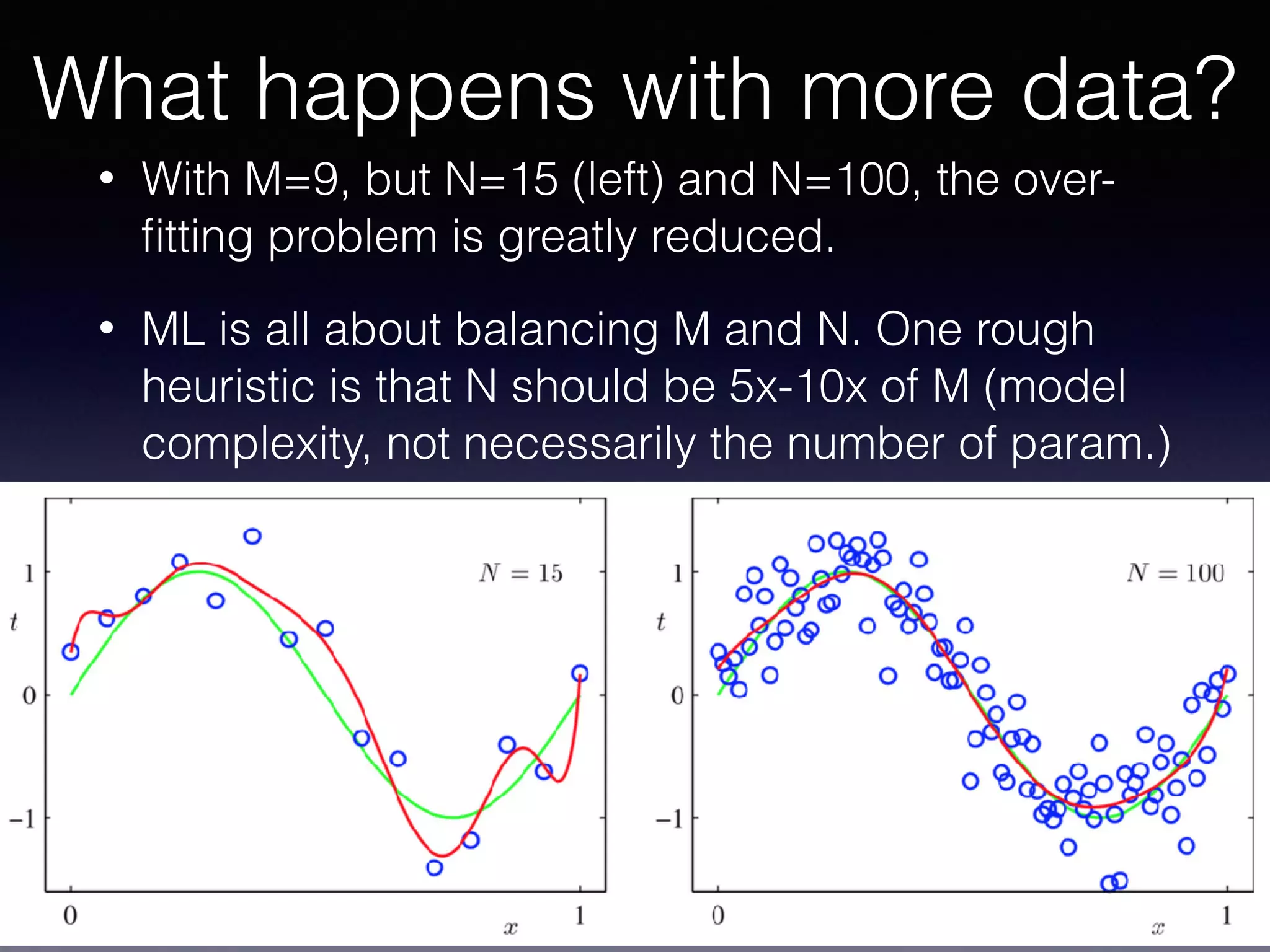

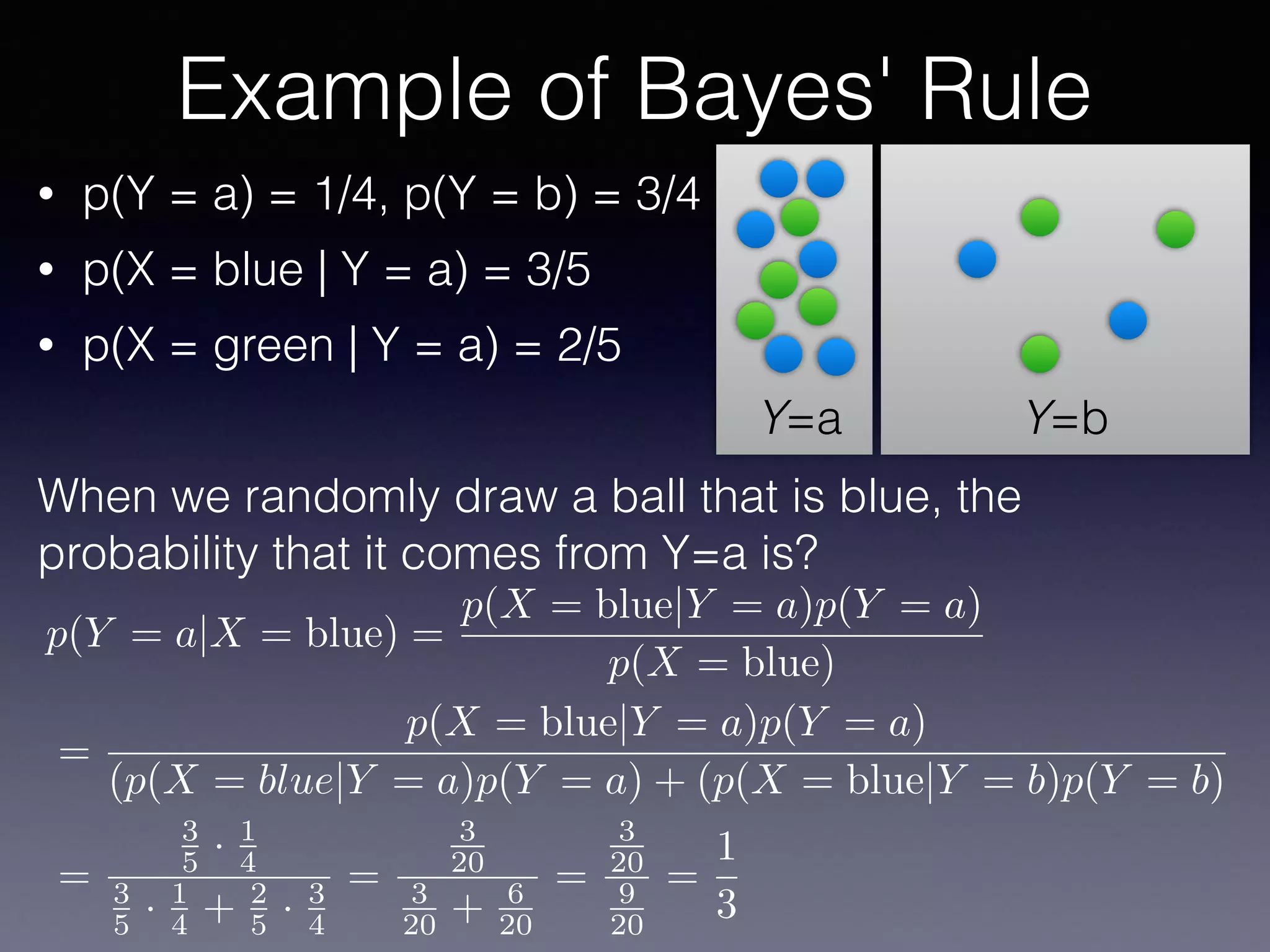
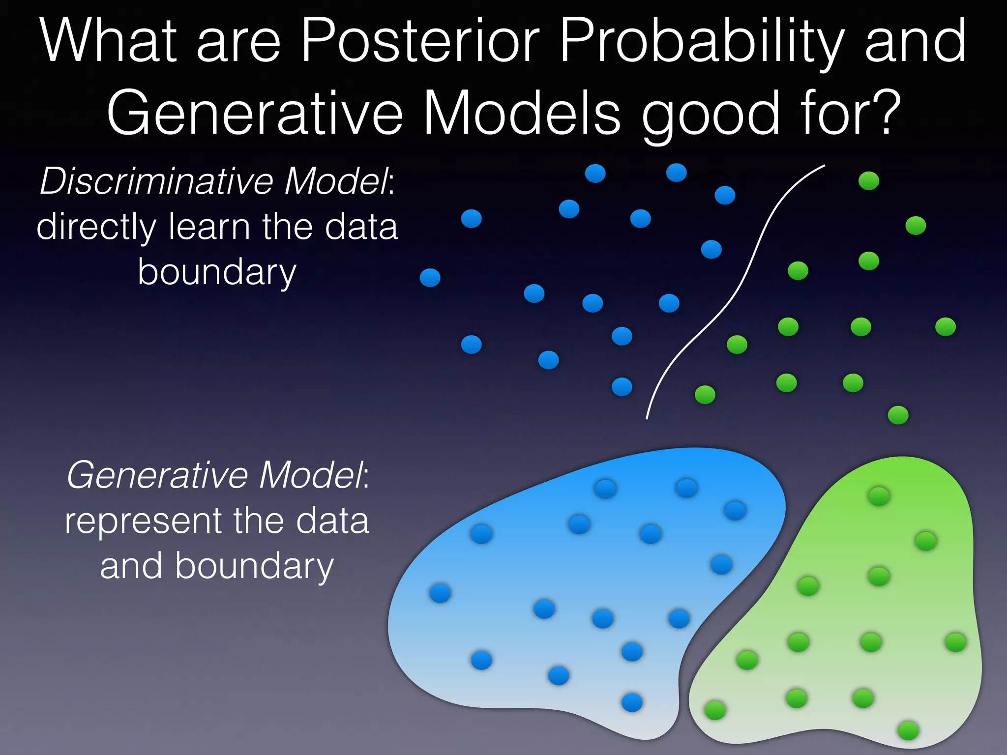
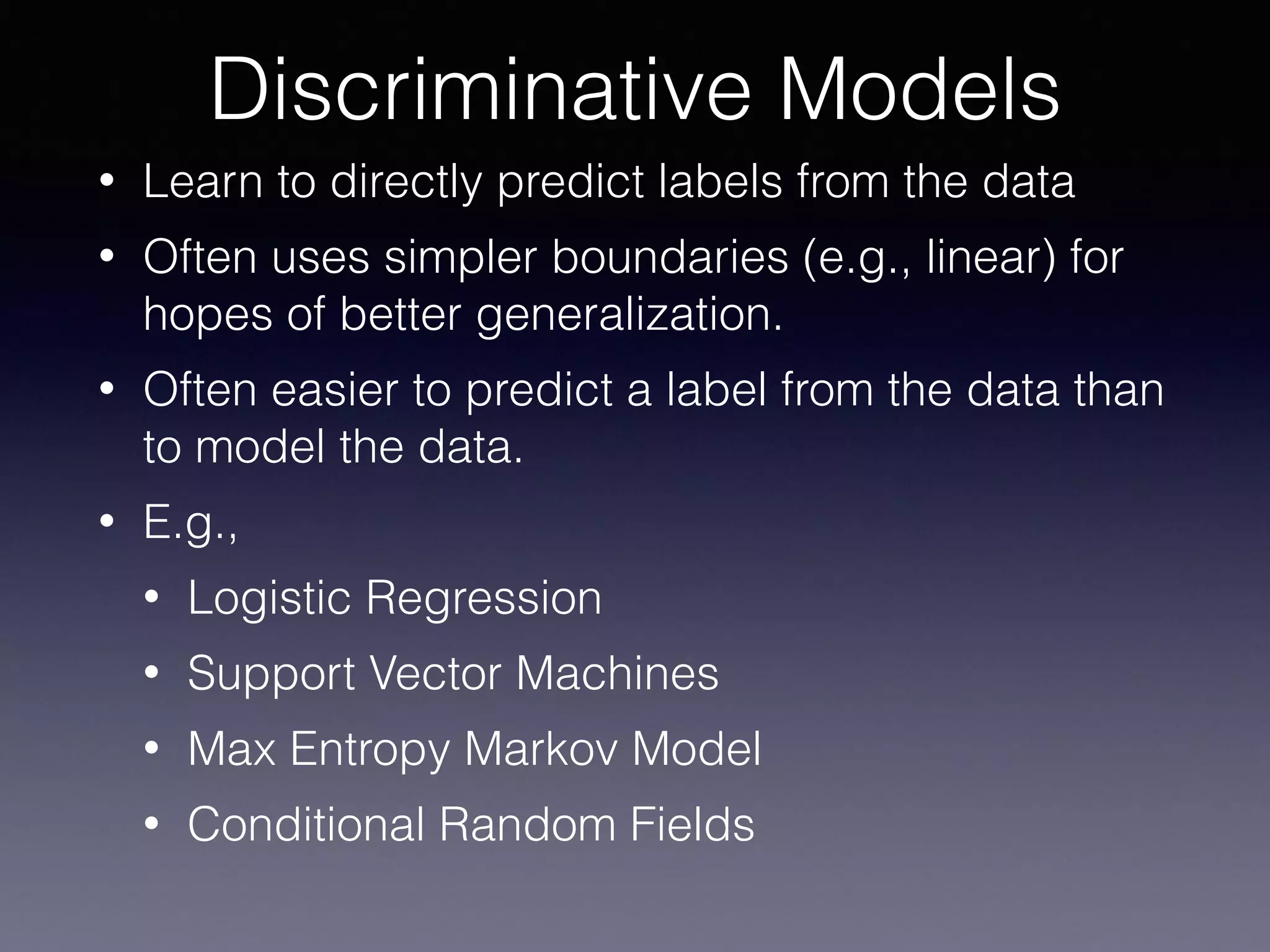
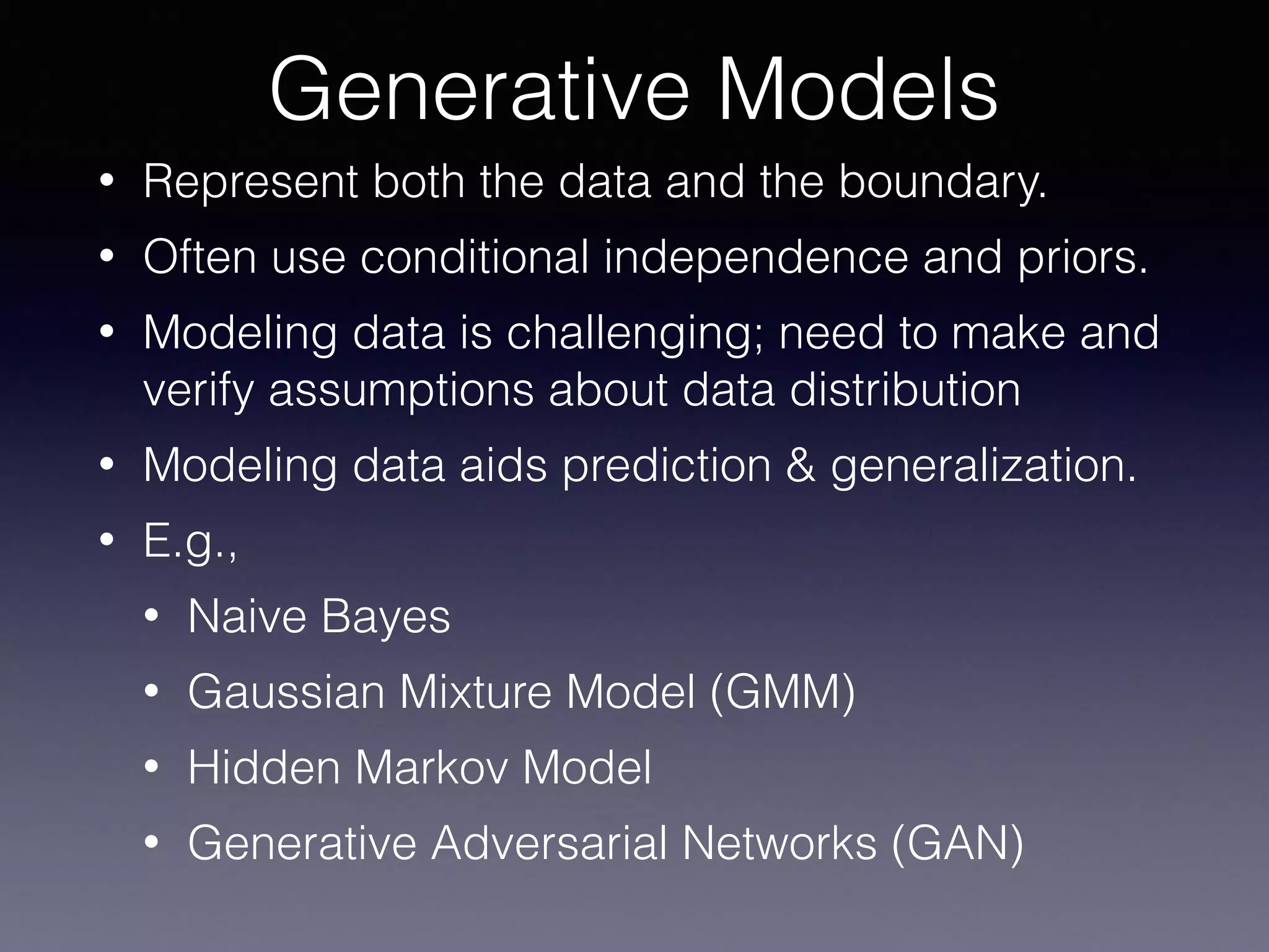


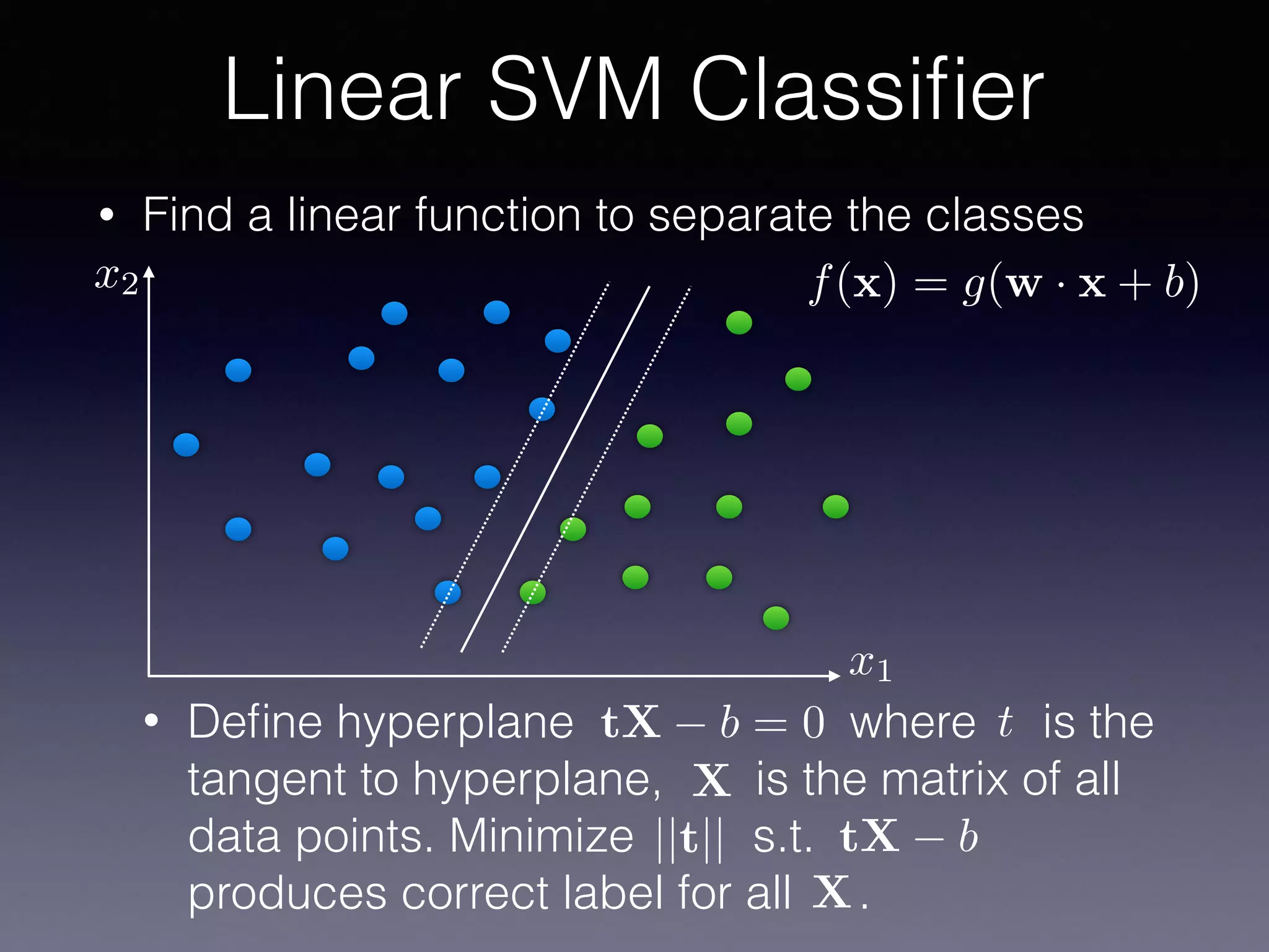
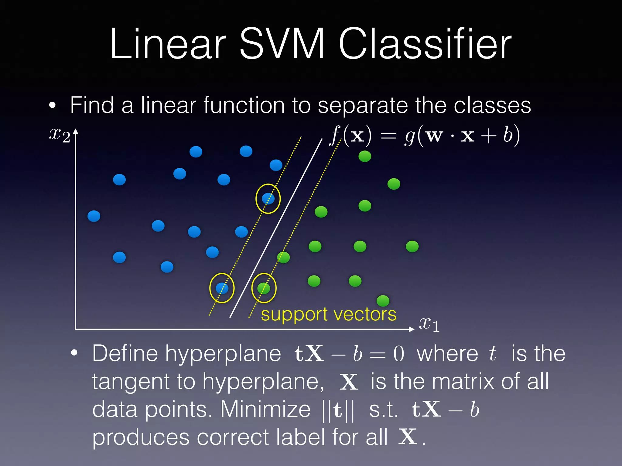
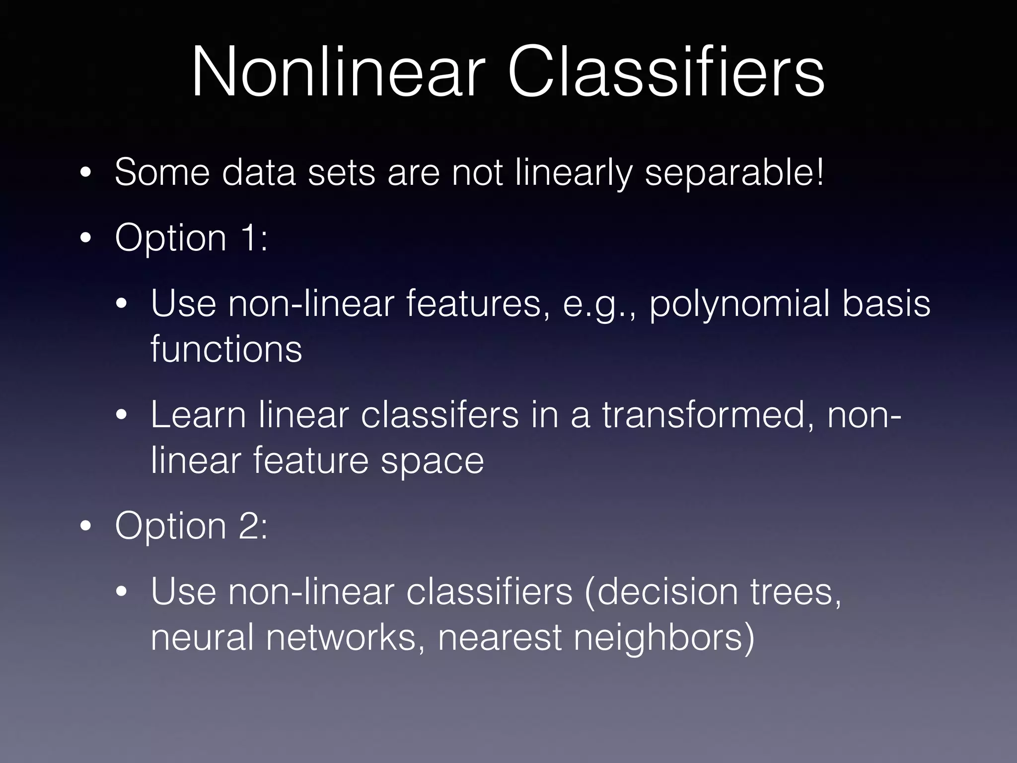
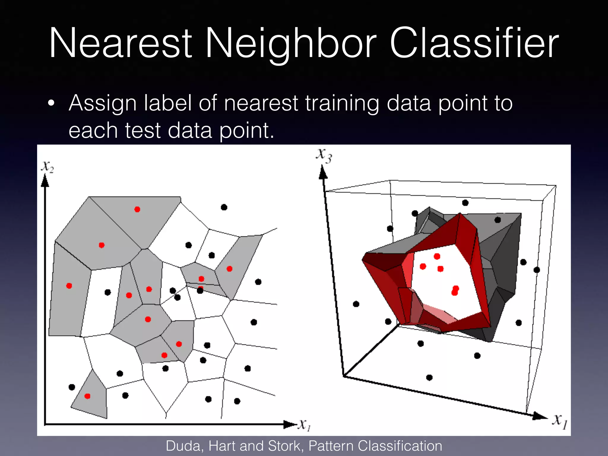


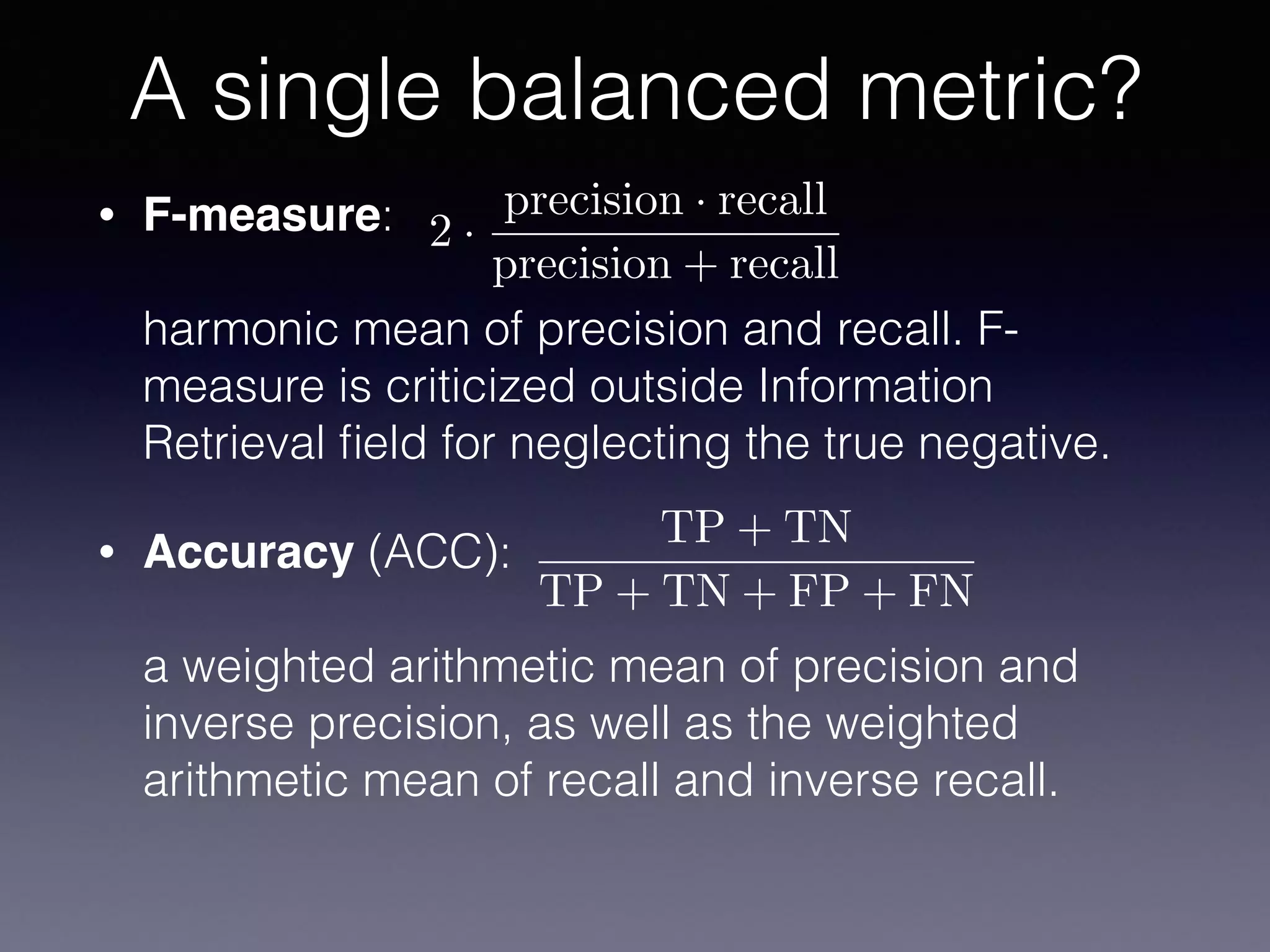
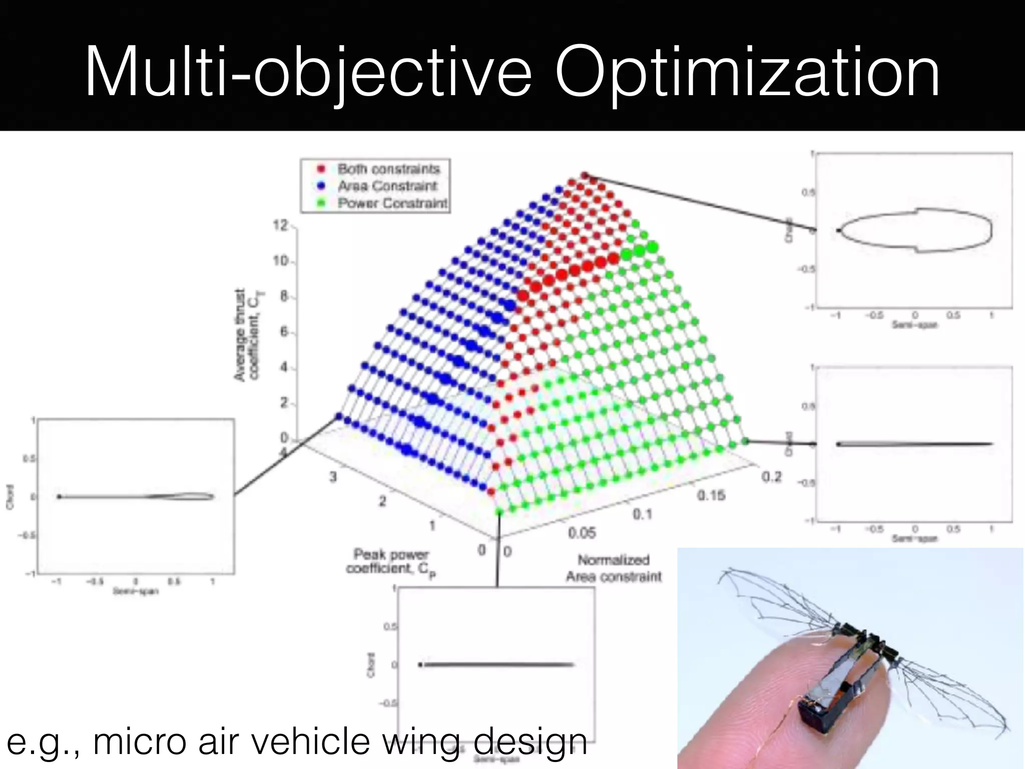
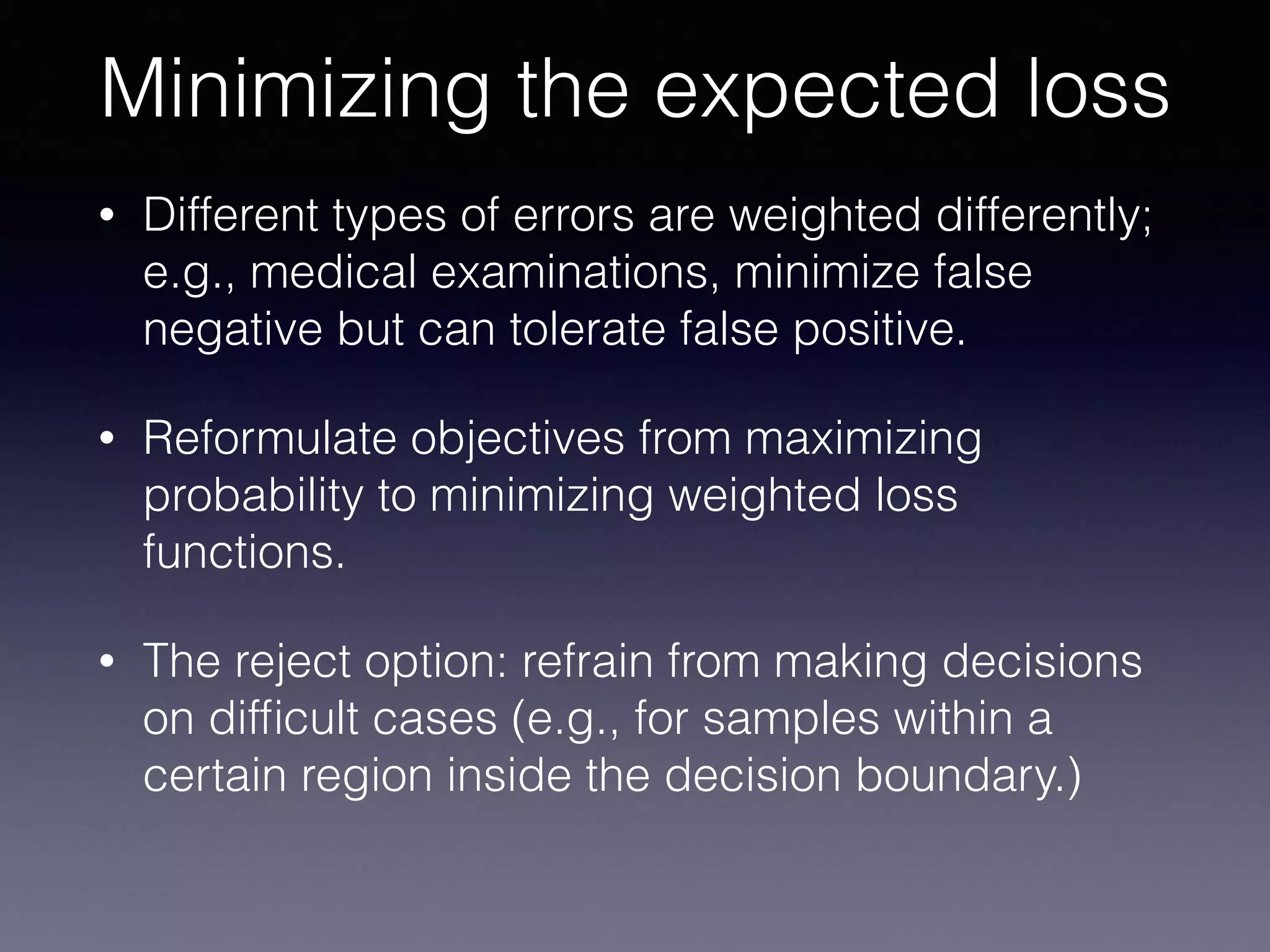
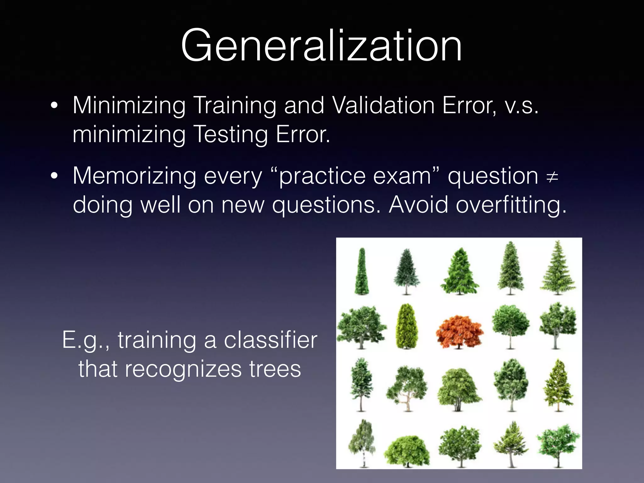


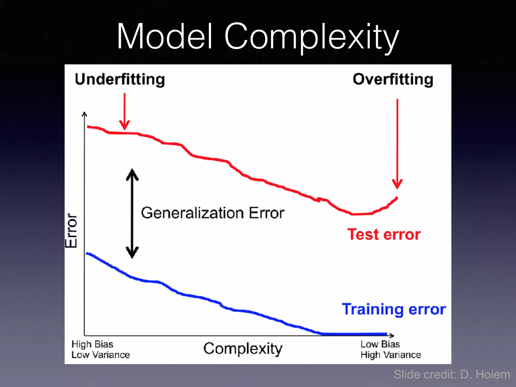
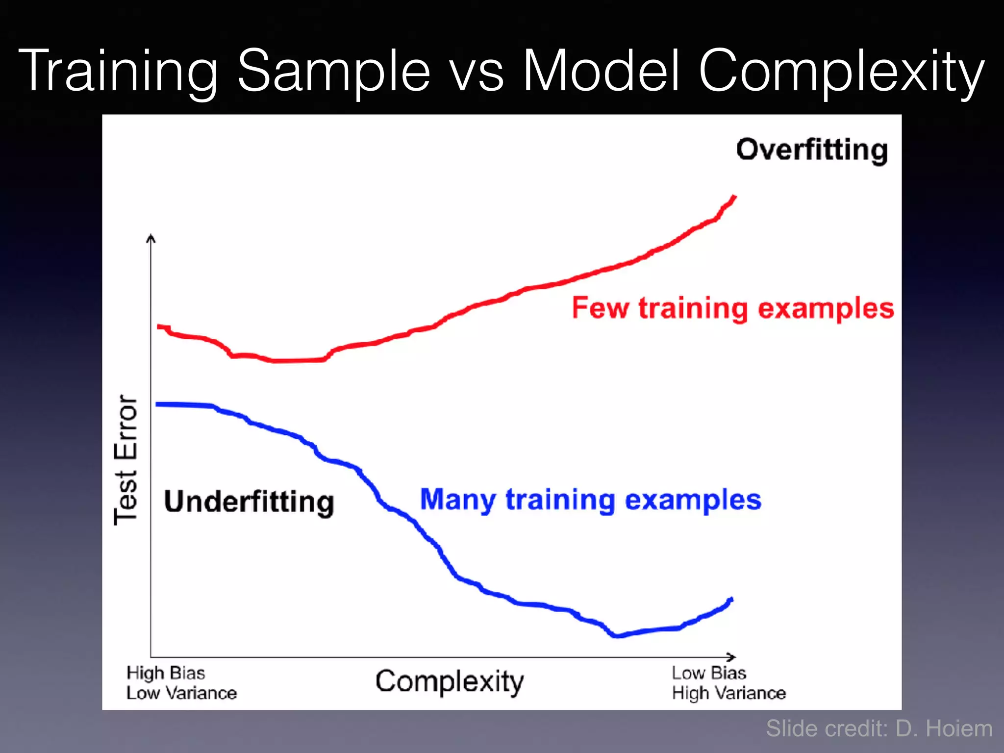
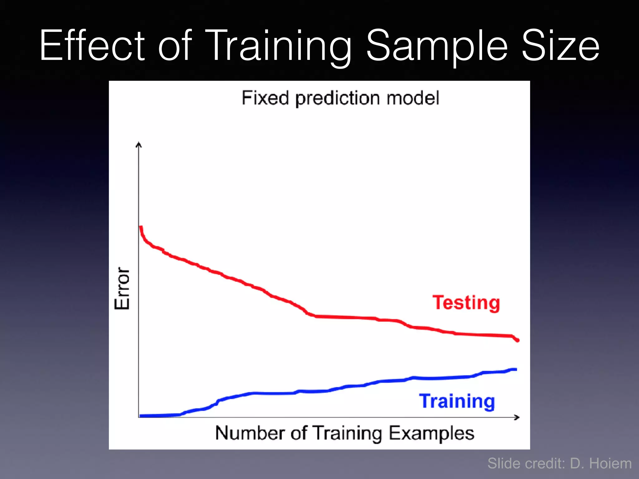
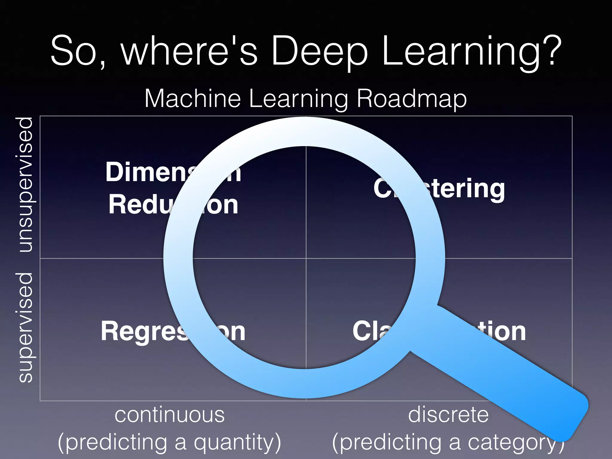
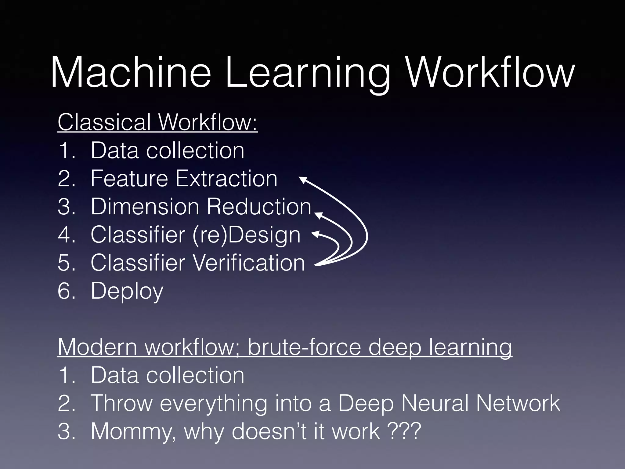
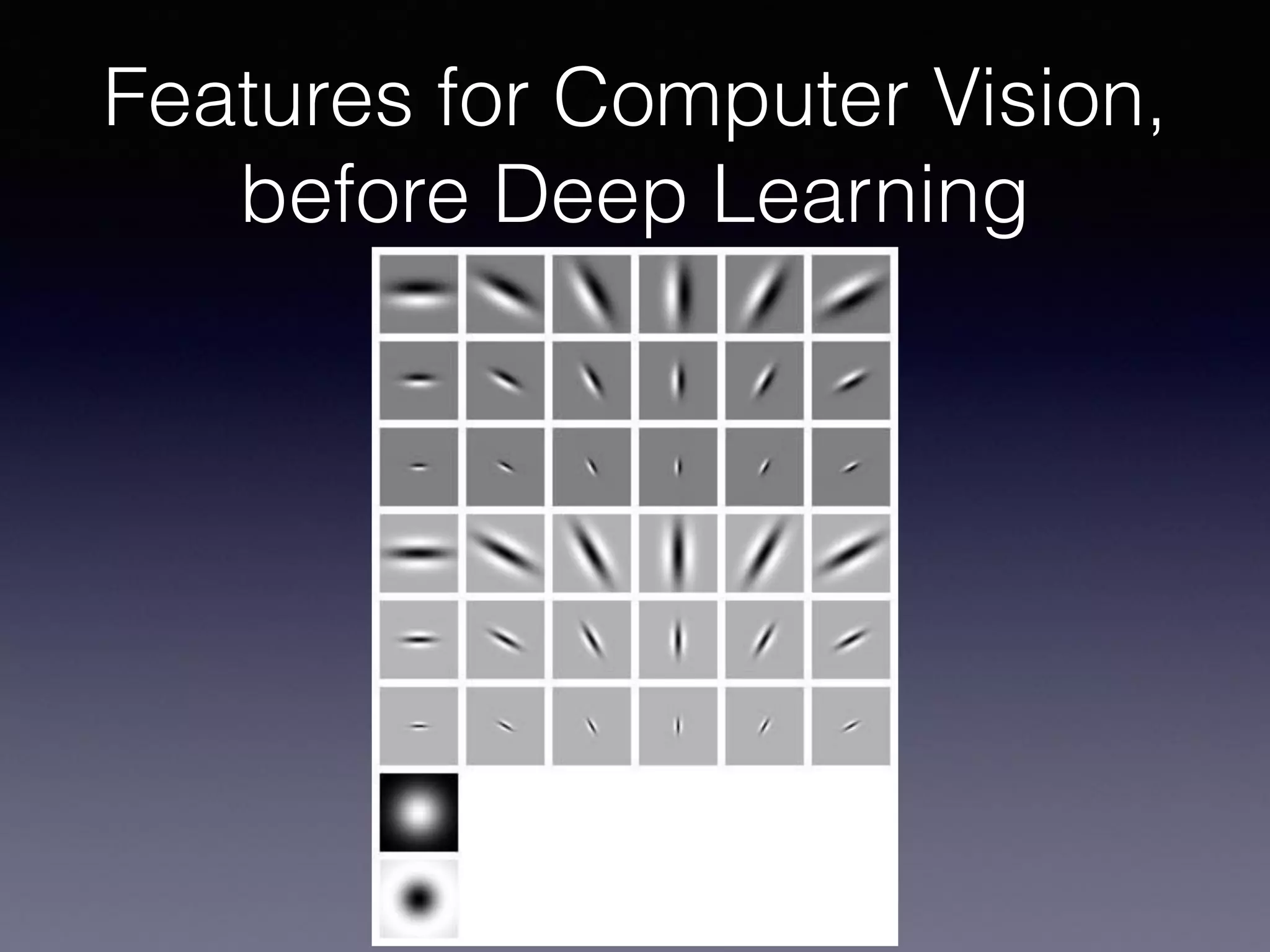
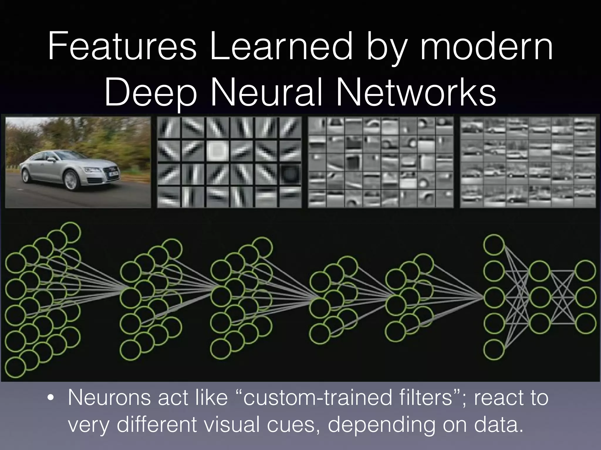
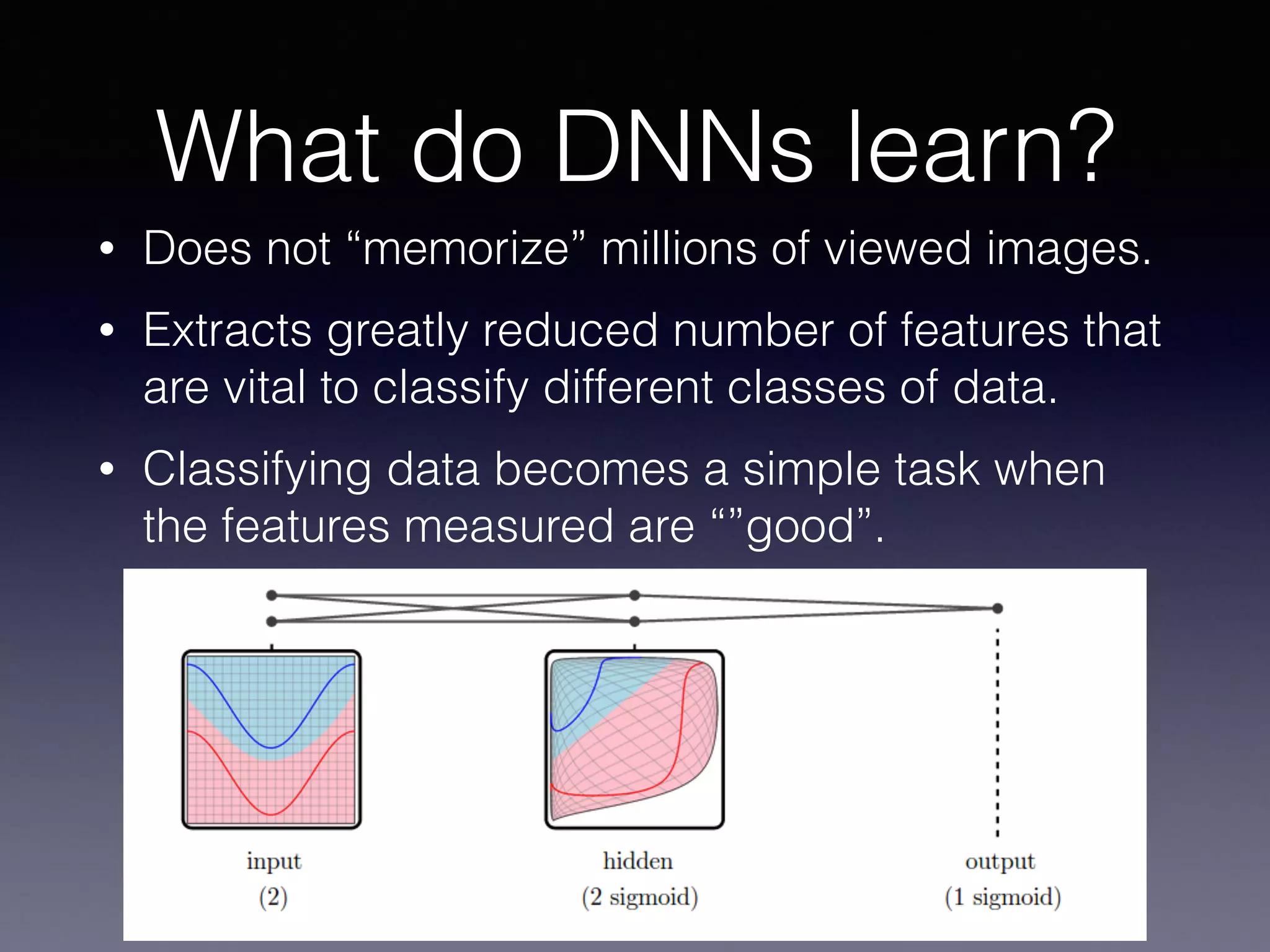


The document outlines the foundational principles of machine learning and artificial intelligence tailored for professional managers, emphasizing the incremental and lean approaches to implementing AI features. It discusses the importance of data cycles, the role of machine learning in varying data scenarios, and the significance of carefully selecting AI features to drive value and reduce risk. Additionally, it provides insights into clustering, dimensionality reduction, and the challenges posed by high-dimensional data in machine learning applications.


![Vibe Coding vs. Spec-Driven Development [Free Meetup]](https://cdn.slidesharecdn.com/ss_thumbnails/vibecodingvsspecdrivendevelopment-251209105622-43f455e7-thumbnail.jpg?width=640&height=640&fit=bounds)


