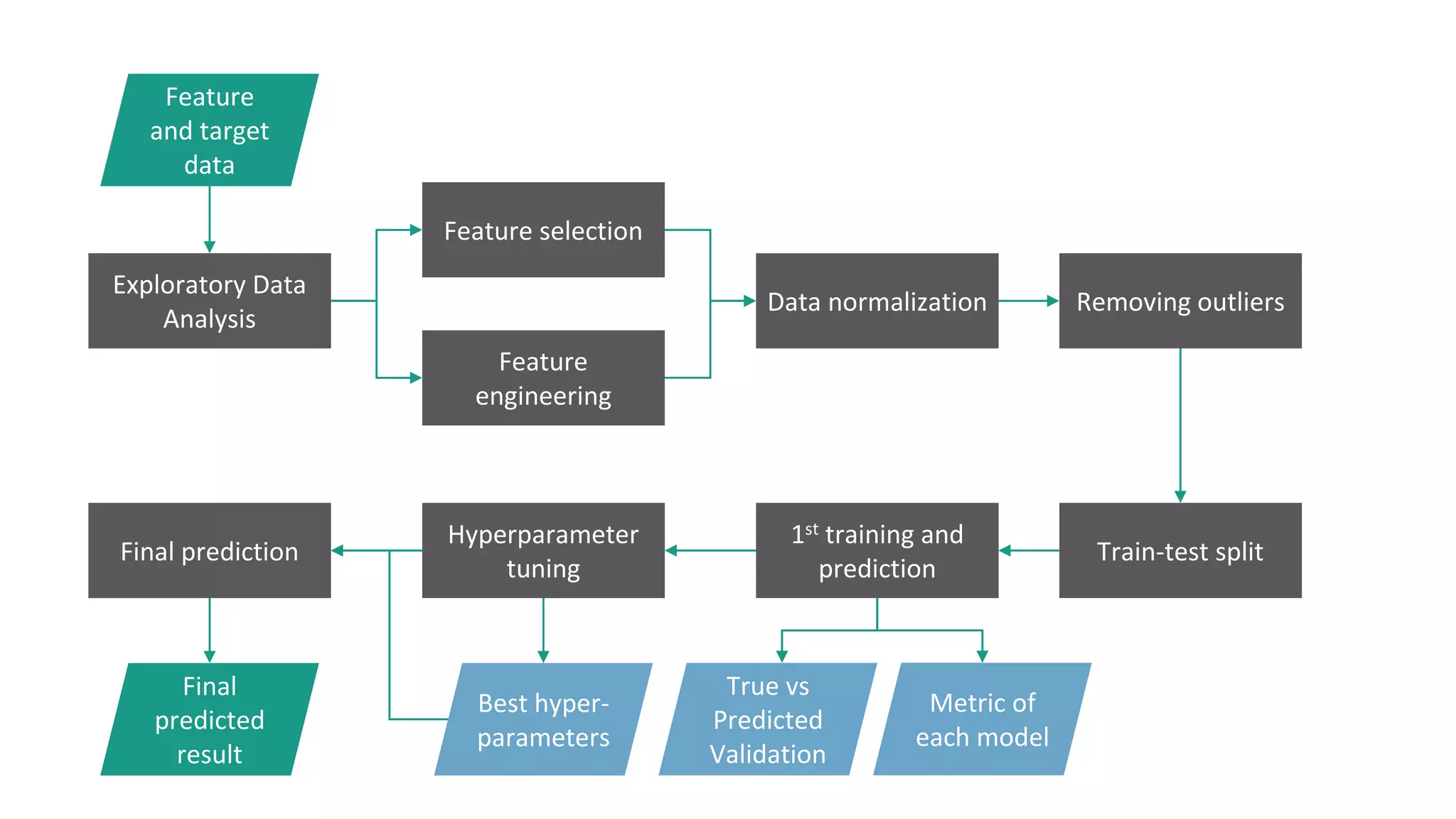
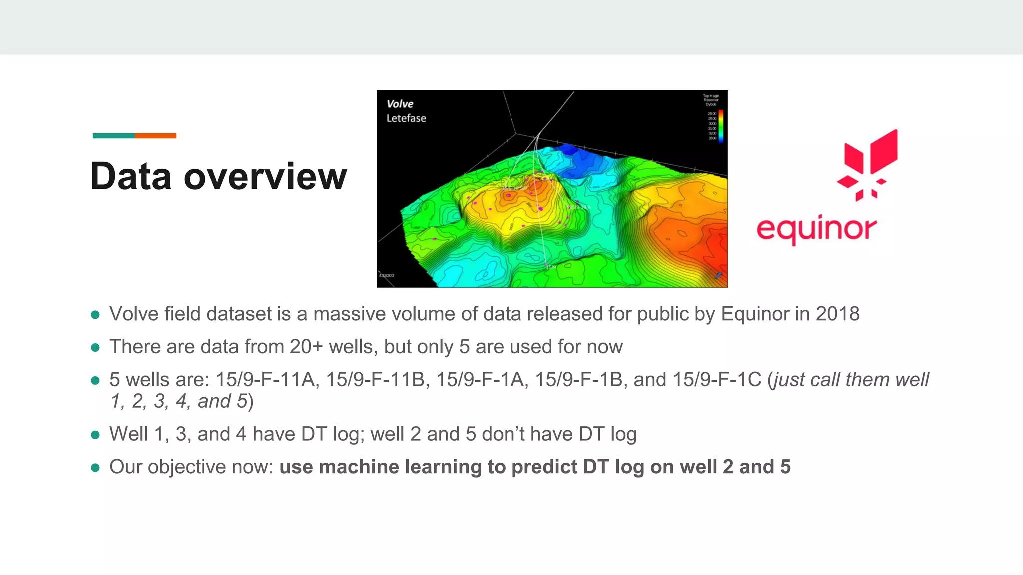
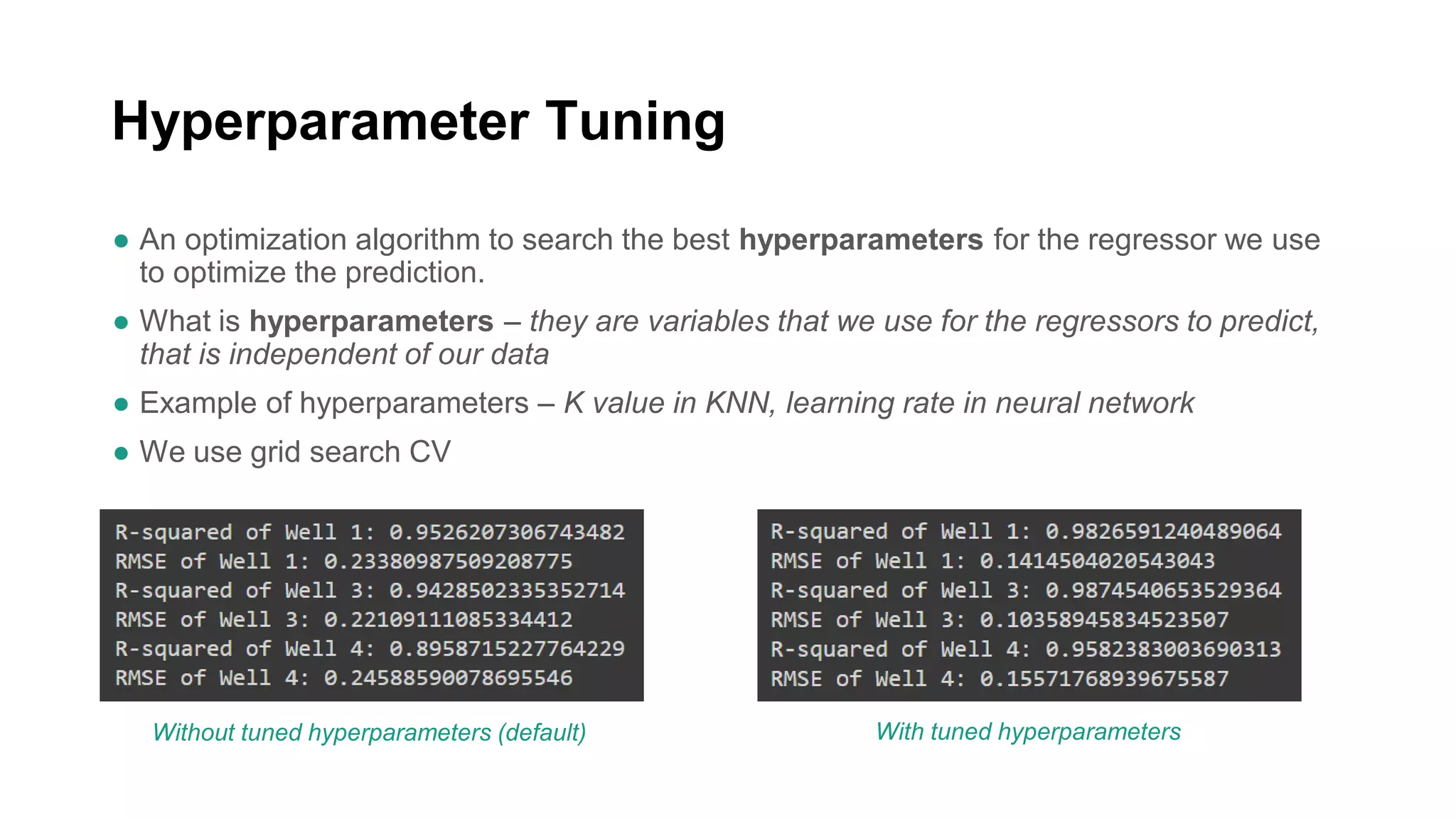
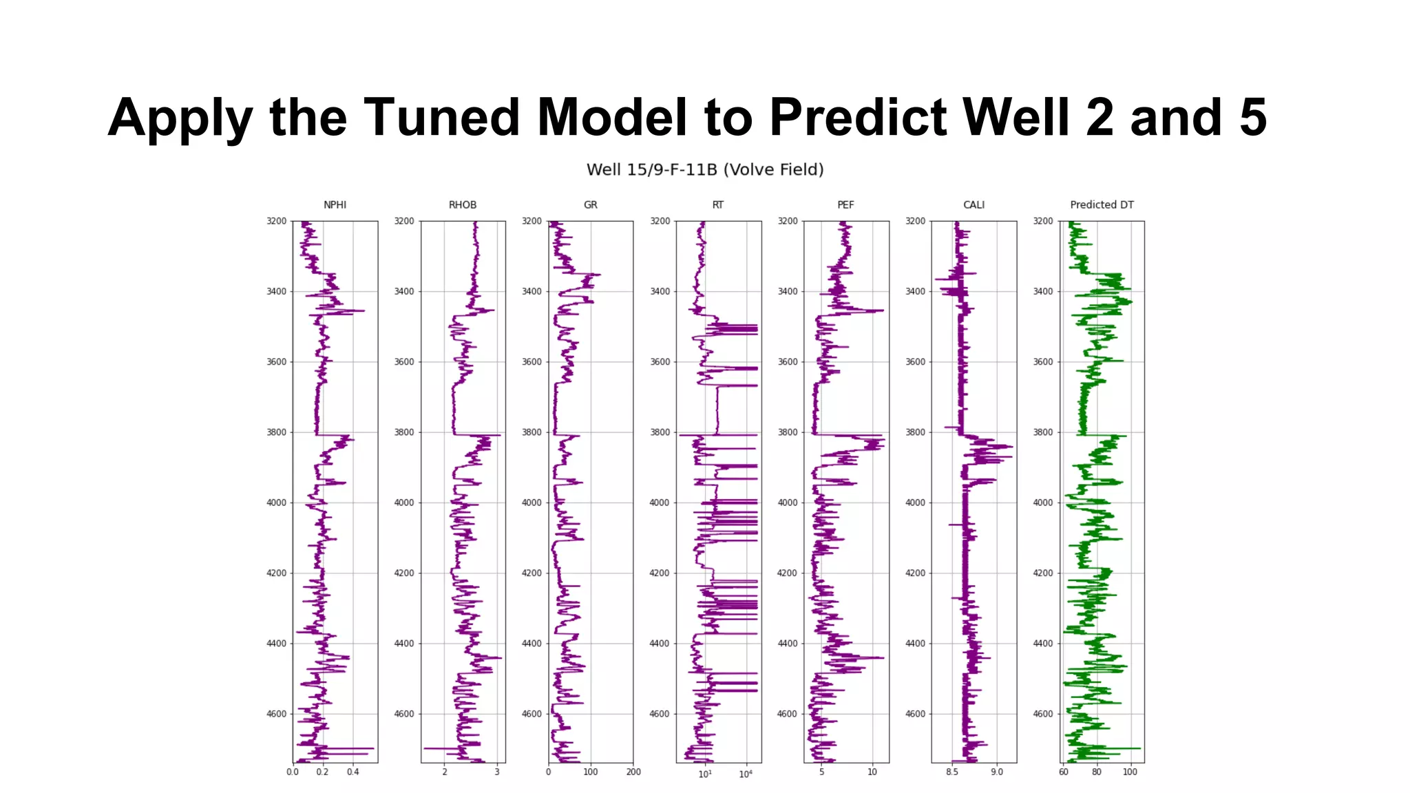
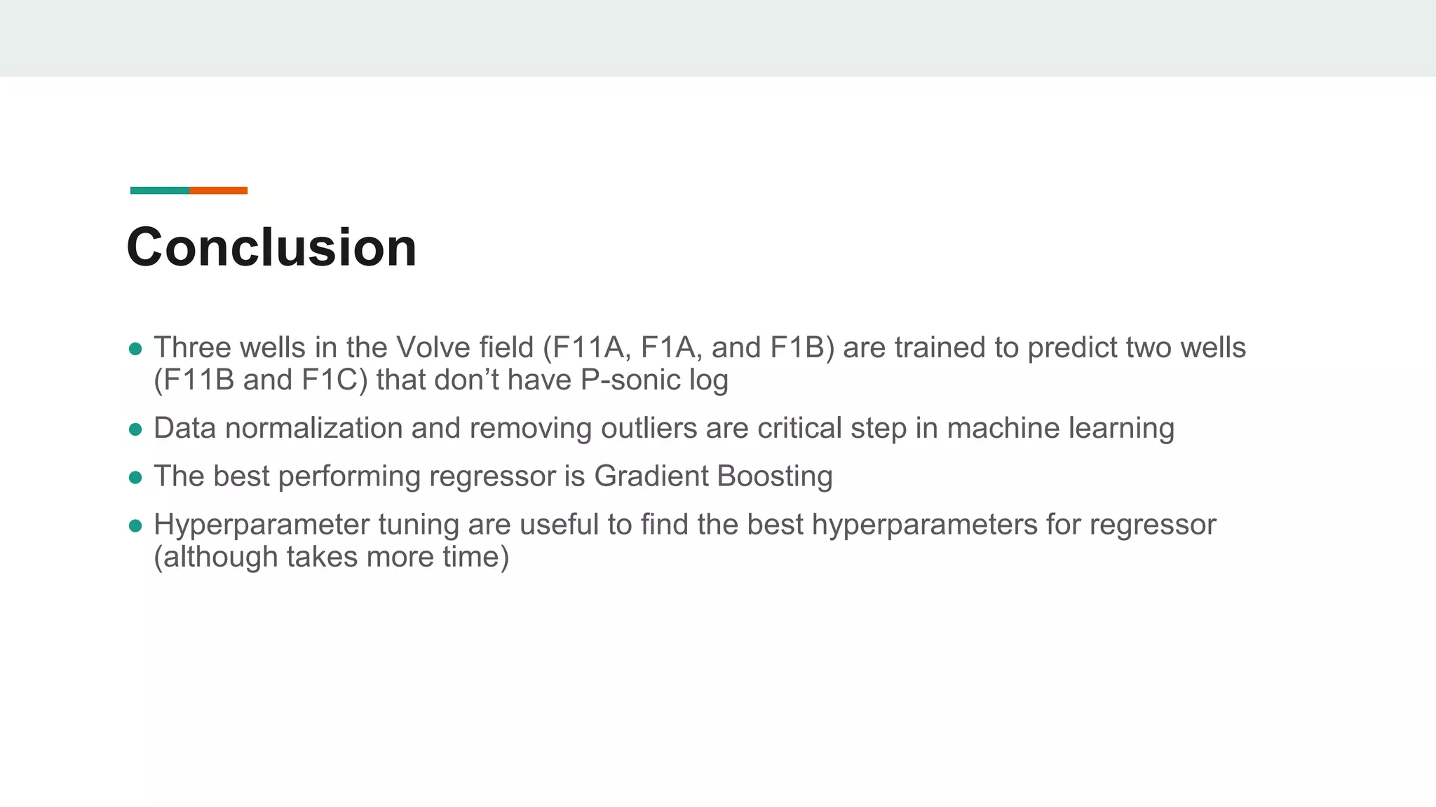
Machine Learning Application in
Subsurface Analysis: Case Study in
the North Sea
Yohanes Nuwara
December 2, 2020
International Geosciences
Symposium
Outlines
● What is Machine Learning ?
● Machine learning in geoscience
● Machine learning workflow
● Case study in Volve field, North Sea
● Exploratory data analysis & Pre-processing
● Prediction
● Conclusion
What is Machine Learning?
● An algorithm-assisted process …
● … that learns through data (as an input),
● … train the data
● … to fit to a mathematical model,
● … and finally output a prediction
Source: Federated Learning (Google AI)
Solving Specific Problems in Geoscience with
ML
● Missing geophysical log traces – supervised learning prediction
● Generating facies model based on geophysical logs from the nearby wells –
supervised learning classification
● Clustering different facies – unsupervised learning classification
● Fault identification – supervised learning (Convolutional Neural Networks / CNN)
● Salt body (or other anomalies e.g. gas chimney) – supervised learning (CNN)
● Rock typing – unsupervised learning (Self Organizing Maps / SOM)
DT
Pred DT
60.2
52.3
51.8
75.2
80.1
49.8
62.1
True DT
60
50
50
70
80
50
60
Machine learning terminologies
● Classification
● Regression
● Training
● Testing
● Supervised
● Unsupervised
● Features
● Target
● Observations
● Continuous
● Categorical
● Non-numerical
values
● Accuracy
Density Resistivity Gamma Ray Formation
2.5 100 80 Heather
2.7 70 Heather
2.2 50 150 Hugin
50 30 Hugin
2.7 75 Hugin
2.2 50 150 Sleipner
50 30 Sleipner
75
55
2.3
2.3
Density Resistivity Gamma Ray Formation
2.5 100 80 Hugin
2.7 30 70 Hugin
2.2 50 150 Hugin
60.2
70.5
82.5
Exploratory Data
Analysis
Feature selection
Feature
engineering
Data normalization Removing outliers
Train-test split
1st training and
prediction
Metric of
each model
Hyperparameter
tuning
True vs
Predicted
Validation
Best hyper-
parameters
Final prediction
Final
predicted
result
Feature
and target
data
Overview of Volve Dataset
Data overview
● Volve field dataset is a massive volume of data released for public by Equinor in 2018
● There are data from 20+ wells, but only 5 are used for now
● 5 wells are: 15/9-F-11A, 15/9-F-11B, 15/9-F-1A, 15/9-F-1B, and 15/9-F-1C (just call them well
1, 2, 3, 4, and 5)
● Well 1, 3, and 4 have DT log; well 2 and 5 don’t have DT log
● Our objective now: use machine learning to predict DT log on well 2 and 5
Well 3 (train)
Well 5
(test)
EDA and Pre-processing
Exploratory Data Analysis 1 (Pairplot)
● Pairplot shows how the data is distributed among itself (univariate) and with one
another (multivariate)
● Diagonal shows the histogram OR “probability density function” (univariate)
● Non-diagonal shows the crossplot of one log and another (multivariate)
Diagonal is the
“probabilistic
density function”
Non-diagonal is the
crossplot between
logs
A
B
C
D
E
F
G
(A) NPHI shows a
left-skewed
distribution
(B) RT shows a
“spike” distribution
(C) Outliers can be
seen
(D) Positive
correlation between
DT and NPHI
(E) Positive
correlation between
RHOB and PEF
(F) Negative
correlation between
RHOB and DT
(G) Less correlation
between DT and
CALI
Exploratory Data Analysis 2 (Heatmap)
● Correlation heatmap shows the correlation between two variables (logs) in a visual way
● Calculate the correlation (2 kinds: Pearson or Spearman)
● Heatmap will tell which features should be phased out – two variables that have LOW
correlation shouldn’t be used as feature for prediction
Pearson’s
correlation
Spearman’s
correlation
Dealing with missing data
● Missing data (NaN; non-numerical value) will be a problem for ML
● 2 ways to handle the missing data:
○ Drop all observations (rows) that have NaN – if we have small dataset, this is not a suggested way
round
○ Impute the NaN with the mean value of the data – also called as imputation
Missing data of facies of 233 wells in the North Sea (below are the 25 wells)
GEOLINK data
Feature engineering
● Feature engineering is a way to transform a variable into a new feature using any
mathematical functions (e.g. log, exponent, etc.) – you can also create new features.
● In petrophysics we know that we’ll visualize RT better if we make it in a semilog plot
● Therefore, we can transform RT into log(RT)
● Then see the new feature using pairplot
Look at this RT now
is better distributed
(no spike anymore)
Data transformation
● Also known as feature scaling
● The objective is to make the distribution be more Gaussian – less skewed
● There are two basic ways: standardization and normalization
● Standardization 🡪 transforming the data by using its standard deviation and average
● Normalization 🡪 transforming the data by using its min and max value
● Other methods such as power transform (box-cox or Yeo-Johnson method) and
regularization (L1 and L2 norm)
● We need to compare which one is the best?
Standardization
(Std and mean)
Focus on the red
box, which one is
more Gaussian?
Power transform
(Yeo-Johnson
method)
Focus on the red
box, which one is
more Gaussian?
Outlier removal
● We saw many outliers in the data
● In fact, machine learning works better if outliers are minimized
● The most basic way to remove outliers is by restricting the data only within the std –
and outside the std, are outliers.
● There are lots of other methods: Isolation Forest, Minimum Covariance (elliptic
envelope method), Local Outlier Factor, and One-class SVM
● Again we compare which one is the best?
Outlier removal
using One-class
SVM
Prediction
Regression models (regressors)
First attempt
● The objective of our 1st attempt is:
○ Compare which regression model is the best to predict DT log
○ Validate our prediction by comparing the true vs. predicted result
● Then, we fit the train data with the regressors, and predict
to the test data – we get the predicted DT
● We compare the true vs. predicted DT of the wells
● We also print metrics (RMSE, R²) to evaluate the
performance of each regressor Well 1
+ Well 3
+ Well 4
Well 1
Well 3
Well 4
Trai
n
Tes
t
Linear regression
SVM
Random Forest
Decision tree
Gradient Boosting
K-Nearest Neighbor
GB
Which one is the best?
● We can see that Gradient Boosting performs the best
● It has the highest R² = 0.95 and lowest RMSE = 0.22
● This is understandable because as per our earlier definition, GB is an ensemble
algorithm that boosts weaker regressors, typically the CART.
● Can we improve performance? – yes, we do hyperparameter tuning
Hyperparameter Tuning
● An optimization algorithm to search the best hyperparameters for the regressor we use
to optimize the prediction.
● What is hyperparameters – they are variables that we use for the regressors to predict,
that is independent of our data
● Example of hyperparameters – K value in KNN, learning rate in neural network
● We use grid search CV
Without tuned hyperparameters (default) With tuned hyperparameters
Apply the Tuned Model to Predict Well 2 and 5
● Three wells in the Volve field (F11A, F1A, and F1B) are trained to predict two wells
(F11B and F1C) that don’t have P-sonic log
● Data normalization and removing outliers are critical step in machine learning
● The best performing regressor is Gradient Boosting
● Hyperparameter tuning are useful to find the best hyperparameters for regressor
(although takes more time)
Conclusion
Thank you
Want to discuss?
E-mail : ign.nuwara97@gmail.com
LinkedIn : https://www.linkedin.com/in/yohanesnuwara/

Machine Learning Applications in Subsurface Analysis: Case Study in North Sea

  • 1.
    Machine Learning Applicationin Subsurface Analysis: Case Study in the North Sea Yohanes Nuwara December 2, 2020 International Geosciences Symposium
  • 2.
    Outlines ● What isMachine Learning ? ● Machine learning in geoscience ● Machine learning workflow ● Case study in Volve field, North Sea ● Exploratory data analysis & Pre-processing ● Prediction ● Conclusion
  • 3.
    What is MachineLearning? ● An algorithm-assisted process … ● … that learns through data (as an input), ● … train the data ● … to fit to a mathematical model, ● … and finally output a prediction Source: Federated Learning (Google AI)
  • 4.
    Solving Specific Problemsin Geoscience with ML ● Missing geophysical log traces – supervised learning prediction ● Generating facies model based on geophysical logs from the nearby wells – supervised learning classification ● Clustering different facies – unsupervised learning classification ● Fault identification – supervised learning (Convolutional Neural Networks / CNN) ● Salt body (or other anomalies e.g. gas chimney) – supervised learning (CNN) ● Rock typing – unsupervised learning (Self Organizing Maps / SOM)
  • 5.
    DT Pred DT 60.2 52.3 51.8 75.2 80.1 49.8 62.1 True DT 60 50 50 70 80 50 60 Machinelearning terminologies ● Classification ● Regression ● Training ● Testing ● Supervised ● Unsupervised ● Features ● Target ● Observations ● Continuous ● Categorical ● Non-numerical values ● Accuracy Density Resistivity Gamma Ray Formation 2.5 100 80 Heather 2.7 70 Heather 2.2 50 150 Hugin 50 30 Hugin 2.7 75 Hugin 2.2 50 150 Sleipner 50 30 Sleipner 75 55 2.3 2.3 Density Resistivity Gamma Ray Formation 2.5 100 80 Hugin 2.7 30 70 Hugin 2.2 50 150 Hugin 60.2 70.5 82.5
  • 6.
    Exploratory Data Analysis Feature selection Feature engineering Datanormalization Removing outliers Train-test split 1st training and prediction Metric of each model Hyperparameter tuning True vs Predicted Validation Best hyper- parameters Final prediction Final predicted result Feature and target data
  • 7.
  • 8.
    Data overview ● Volvefield dataset is a massive volume of data released for public by Equinor in 2018 ● There are data from 20+ wells, but only 5 are used for now ● 5 wells are: 15/9-F-11A, 15/9-F-11B, 15/9-F-1A, 15/9-F-1B, and 15/9-F-1C (just call them well 1, 2, 3, 4, and 5) ● Well 1, 3, and 4 have DT log; well 2 and 5 don’t have DT log ● Our objective now: use machine learning to predict DT log on well 2 and 5
  • 9.
  • 10.
  • 11.
  • 12.
    Exploratory Data Analysis1 (Pairplot) ● Pairplot shows how the data is distributed among itself (univariate) and with one another (multivariate) ● Diagonal shows the histogram OR “probability density function” (univariate) ● Non-diagonal shows the crossplot of one log and another (multivariate)
  • 13.
    Diagonal is the “probabilistic densityfunction” Non-diagonal is the crossplot between logs A B C D E F G (A) NPHI shows a left-skewed distribution (B) RT shows a “spike” distribution (C) Outliers can be seen (D) Positive correlation between DT and NPHI (E) Positive correlation between RHOB and PEF (F) Negative correlation between RHOB and DT (G) Less correlation between DT and CALI
  • 14.
    Exploratory Data Analysis2 (Heatmap) ● Correlation heatmap shows the correlation between two variables (logs) in a visual way ● Calculate the correlation (2 kinds: Pearson or Spearman) ● Heatmap will tell which features should be phased out – two variables that have LOW correlation shouldn’t be used as feature for prediction Pearson’s correlation Spearman’s correlation
  • 16.
    Dealing with missingdata ● Missing data (NaN; non-numerical value) will be a problem for ML ● 2 ways to handle the missing data: ○ Drop all observations (rows) that have NaN – if we have small dataset, this is not a suggested way round ○ Impute the NaN with the mean value of the data – also called as imputation
  • 17.
    Missing data offacies of 233 wells in the North Sea (below are the 25 wells) GEOLINK data
  • 18.
    Feature engineering ● Featureengineering is a way to transform a variable into a new feature using any mathematical functions (e.g. log, exponent, etc.) – you can also create new features. ● In petrophysics we know that we’ll visualize RT better if we make it in a semilog plot ● Therefore, we can transform RT into log(RT) ● Then see the new feature using pairplot
  • 19.
    Look at thisRT now is better distributed (no spike anymore)
  • 20.
    Data transformation ● Alsoknown as feature scaling ● The objective is to make the distribution be more Gaussian – less skewed ● There are two basic ways: standardization and normalization ● Standardization 🡪 transforming the data by using its standard deviation and average ● Normalization 🡪 transforming the data by using its min and max value ● Other methods such as power transform (box-cox or Yeo-Johnson method) and regularization (L1 and L2 norm) ● We need to compare which one is the best?
  • 21.
    Standardization (Std and mean) Focuson the red box, which one is more Gaussian?
  • 22.
    Power transform (Yeo-Johnson method) Focus onthe red box, which one is more Gaussian?
  • 23.
    Outlier removal ● Wesaw many outliers in the data ● In fact, machine learning works better if outliers are minimized ● The most basic way to remove outliers is by restricting the data only within the std – and outside the std, are outliers. ● There are lots of other methods: Isolation Forest, Minimum Covariance (elliptic envelope method), Local Outlier Factor, and One-class SVM ● Again we compare which one is the best?
  • 24.
  • 25.
  • 26.
  • 27.
    First attempt ● Theobjective of our 1st attempt is: ○ Compare which regression model is the best to predict DT log ○ Validate our prediction by comparing the true vs. predicted result ● Then, we fit the train data with the regressors, and predict to the test data – we get the predicted DT ● We compare the true vs. predicted DT of the wells ● We also print metrics (RMSE, R²) to evaluate the performance of each regressor Well 1 + Well 3 + Well 4 Well 1 Well 3 Well 4 Trai n Tes t
  • 28.
    Linear regression SVM Random Forest Decisiontree Gradient Boosting K-Nearest Neighbor
  • 29.
  • 30.
    Which one isthe best? ● We can see that Gradient Boosting performs the best ● It has the highest R² = 0.95 and lowest RMSE = 0.22 ● This is understandable because as per our earlier definition, GB is an ensemble algorithm that boosts weaker regressors, typically the CART. ● Can we improve performance? – yes, we do hyperparameter tuning
  • 31.
    Hyperparameter Tuning ● Anoptimization algorithm to search the best hyperparameters for the regressor we use to optimize the prediction. ● What is hyperparameters – they are variables that we use for the regressors to predict, that is independent of our data ● Example of hyperparameters – K value in KNN, learning rate in neural network ● We use grid search CV Without tuned hyperparameters (default) With tuned hyperparameters
  • 32.
    Apply the TunedModel to Predict Well 2 and 5
  • 33.
    ● Three wellsin the Volve field (F11A, F1A, and F1B) are trained to predict two wells (F11B and F1C) that don’t have P-sonic log ● Data normalization and removing outliers are critical step in machine learning ● The best performing regressor is Gradient Boosting ● Hyperparameter tuning are useful to find the best hyperparameters for regressor (although takes more time) Conclusion
  • 34.
    Thank you Want todiscuss? E-mail : ign.nuwara97@gmail.com LinkedIn : https://www.linkedin.com/in/yohanesnuwara/