This document describes a Bayesian adaptive dose selection procedure using semi-parametric dose-response modeling. It involves modeling dose-response relationships non-parametrically using a monotonicity constraint, applying Bayesian model averaging over different dose-response shapes, and performing predictive probability calculations using importance sampling to determine the dose to take forward at an interim analysis based on predictive probabilities of success criteria being met. Simulation results demonstrate the procedure can correctly identify the optimal dose and uses fewer patients than a non-adaptive design.

1. A Bayesian Adaptive Dose Selection Procedure with
Semi-Parametric Dose-Response Modeling
Luca Pozzi
University of California, Berkeley
p.luc@stat.berkeley.edu
January 24, 2012 - 5th Annual Bayesian Biostatistics Conference, Houston, TX

2. Predictive Probability in Clinical Trials
Berry et al. 2010, Chapter 4
“The Predictive Probability approach looks into the future based on
the current observed data to project whether a positive conclusion
at the end of the study is likely or not, and then makes a sensible
decision at the present time accordingly.”

3. Predictive Probability of Success (PPS)
For the ease of notation let us define:
Y = {Past Data} i.e. interim data;
Y ∗ = {Future Data} i.e. post interim data.
In our setting, as in Berry et al. (2010)
PPS = P{Success|Y } = P{Y ∗ ∈ YS |Y } = p (Y ∗ |Y )dY ∗ (1)
YS
being YS defined as
{Success} = YS = {Y ∗ : P{θ ∈ ΘE |Y ∗ , Y } > t }
for some efficacy domain ΘE and some threshold t, the predictive quantity (??)
then becomes
PPS = 1{P{θ ∈ ΘE |Y ∗ , Y } > t }p (Y ∗ |Y )dY ∗ (2)
where P{θ ∈ ΘE |Y ∗ , Y } = ΘE
p (θ|Y ∗ , Y )dθ.

4. Motivating Example: Problem Setting
Objective: Lowest Effective Dose (LED), i.e. dose whose efficacy is
at least 50% better than placebo (Dose 1) and
at most 20% worse than the highest dose (Dose 5);
Design of the Study: Start with initial allocation 1:a:b:c:1 then at interim
stop or select the most promising dose d for a second
phase with only placebo, Dose d and Dose 5;
Endpoint: Overdispersed count data Y modeled by the negative
binomial distribution (Gamma-Poisson mixture):
Y |λ ∼ Pois(λ)
λ|(α, β) ∼ Gamma(α, β)
Pharmacodynamic: Sigmoidal relationship
EMAX ·D
e.g. EMAX -model: E (D ) = E0 1 − D50% +D
.
Strong prior information available for placebo (E0 ) and
highest dose (EMAX );

5. Modeling Dose-Response Relationship
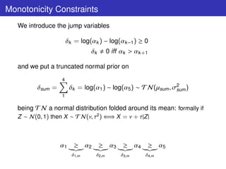
1st challenge: Modeling
Too few doses to adopt Parametric Dose-Response model.
(Adaptive design will start with only one lower dose)
Strategy: Semiparametric Specification
The mode of action of the drug and Ph.III outcomes suggest that a
monotonicity constraint holds for the dose-response relationship:
Mm = µj ≡ E[Yij ] : E0 = µ1 ≥ µ2 ≥ µ3 ≥ µ4 ≥ µ5 = EMAX

6. Modeling Approach
Bayesian Model Averaging: Ingredients
1 A set of mutually exclusive models M = {M1 , ..., MM }.
To each model corresponds a probability distribution
f (y |θ(m) , Mm );
2 One set of priors g (θ(m) |Mm ) on θ(m) for each Mm ;
3 A vector of prior model probabilities π = (π1 , ..., πM ), πm = P{Mm },
(e.g. πm = M ), ∀ m = 1, ..., M.
1
We have then:
M
P{success|y } = P{success|Mm , y }P{Mm |y }
m=1

7. Bayesian model
Gamma-Poisson:
for the i-th patient and the j-th dose group
Yij |λij ∼ dpois(λij )
λij |αj , β ∼ dgamma(αj , β)
So Yij marginal distribution is a dnegbin(αj , β)
Priors:
log(α1 ) ∼ N(µα , σ2 );
α
α|m ∼ fm λd (m)
log(β) ∼ N(0, σ2 )
β

8. Monotonicity Constraints
We introduce the jump variables
δk = log(αk ) − log(αk −1 ) ≥ 0
δk 0 iff αk > αk +1
and we put a truncated normal prior on
4
δsum = δk = log(α1 ) − log(α5 ) ∼ T N(µsum , σ2 )
sum
1
being T N a normal distribution folded around its mean: formally if
Z ∼ N(0, 1) then X ∼ T N(ν, τ2 ) ⇐⇒ X = ν + τ|Z |
α1 ≥ α2 ≥ α3 ≥ α4 ≥ α5
δ1,m δ2,m δ3,m δ4,m

9. Jump×Model Matrix
 δ1,1 0 δ1,3 δ1,4 0 0 δ1,10
 
 0 0 0 

 δ
 2,1 δ2,2 δ2,3 δ2,4 0 δ2,6 0 δ2,8 0

0



∆=
 

 δ
 3,1 δ3,2 δ3,3 0 δ3,5 δ3,6 0


 0 δ3,9 0





 
δ4,1 δ4,2 0 0 δ4,5 0 δ4,7
 
0 0 0
e.g. M5 : µ1 = µ2 = µ3 > µ4 > µ5
α1 = α2 = α3 > α4 > α5
δ3,5 δ4,5

10. Criteria
Futility-Success
Exclusion Criterion P{µd /µ1 ≥ 0.7|data} ≥ 50%, i.e. Dose d is not
superior to placebo.
Efficacy Criterion is the intersection of the following events:
(i) the dose is far enough from Dose 1
P{µd /µ1 < 1|data} ≥ 95%
(ii) the dose is either at least 50% better than
Dose 1, or at most 20% worse than Dose 5.
P{µd /µ1 ≤ 0.5|data}
max ≥ 50%
P{µd /µ5 ≤ 1.2|data}

11. Interim Decision
At Interim
• if Dose 4 meets Exclusion Criterion stop for futility: no dose
lower than Dose 5 is effective;
• if Dose 2 meets Efficacy Criteria stop for success: Dose 2 is
the LED;
• otherwise, for each not futile Dose d calculate the Predictive
Probability of Success (PPS) and allocate to the lowest
dose for which
P (i) Ad , Y , Y ∗ ∩ (ii) Ad , Y , Y ∗ > 50% Y ≥ t (3)
with Ad = {allocate to Dose d }.

12. Decision Tree
LED = d3
LED = d4
A4
LED = d2
LED
LED = d4
LED = d5
LED
Start the Trial Decision at Interim A3
LED = d2
LED = d2
LED = d3
LED = d2
LED
A2
LED = d3
LED = d4

13. Performing Predictive Probability Calculations
2nd challenge: Computational
Not feasible to use WinBUGS for Predictive Calculations
Stategy: Importance Sampling
Sample from the posterior sample using weighted resampling:
(α, β)(1) , ..., (α, β)(N ) → (α, β)∗

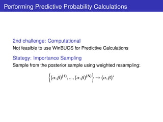
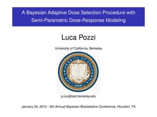
14. Algorithm: Predictive Resample
1 Sample (α, β)(1) , ..., (α, β)(k ) , ..., (α, β)(N ) ;
2 Select Dose d;
3 for l = 1, ..., L draw (α, β)(l ) from the posterior sample at
interim of size N;
∗(l )
4 Simulate one dataset Yd |(α, β)(l ) , Ad ;
SIR
(l )
5 Compute p Yd |(α, β)(k ) , k = 1, ..., N;
∗(l )
l (θk ;Y ∗ ) p (Yd |(α,β)(k ) )
6 Compute wk = ∗ = ∗(l ) ;
j l (θj ;Y ) j p (Yd |(α,β)(j ) )
(l )
7 Compute by resampling PPd [criterion] for each criteria;
In the end:
L
 
1 (l )
{PPd [criterion] c }

 

PPd = mean







{criteria} l =1

15. Dose-Response Relationships
Optimistic Scenario Flat a Flat b
1.0
1.0
1.0
0.8
0.8
0.8
0.6
0.6
0.6
α
α
α
0.4
0.4
0.4
0.2
0.2
0.2
0.0
0.0
0.0
d1 d2 d3 d4 d5 d1 d2 d3 d4 d5 d1 d2 d3 d4 d5
dose dose dose
Pessimistic Scenario Moderate Scenario Borderline Moderate Scenario
1.0
1.0
1.0
0.8
0.8
0.8
0.6
0.6
0.6
α
α
α
0.4
0.4
0.4
0.2
0.2
0.2
0.0
0.0
0.0
d1 d2 d3 d4 d5 d1 d2 d3 d4 d5 d1 d2 d3 d4 d5
dose dose dose
Red represents the real LED (“right” dose).

16. Simulation Setup
Initial Allocation: assuming we start with 1 : a : b : c : 1:
• a = 0, b = 1, c = 0, i.e. 1:0:1:0:1;
• a = 1, b = 1, c = 1, i.e. 1:1:1:1:1;
• a = 1, b = 2, c = 1, i.e. 1:1:2:1:1.
 0.4


Predictive Probability Threshold: t =  0.5



 0.6

Number of Patients: split the 250 patients between the first and
the second phase:
• 30% at interim and 70% for the next phase;
• half at interim and half for the next phase.
Size: 500 simulations with 500 simulated studies for
prediction and N = 104 for the resampling.

17. Operation Characteristics (Adaptive Design)
Moderate Scenario
Let us consider P{ “right” dose} in the Moderate Scenario:
1:0:1:0:1 1:1:1:1:1 1:1:2:1:1
0.4 0.5 0.6 0.4 0.5 0.6 0.4 0.5 0.6
50% 0.818 0.878 0.996 0.774 0.818 0.768 0.730 0.794 0.848
30% 0.860 0.860 0.996 0.818 0.858 0.814 0.734 0.780 0.864
Performances of Non-Adaptive design
Optimistic Moderate Flat(a) Flat(b) Pessimistic
P{right dose} 0.982 0.84 0.26675 0.3924688 0.94
P{Success} 1.000 1.00 0.36775 0.6775810 0.06

18. Operation Characteristics: Cheaper Solution
Expected number of patients (total sample size = 250)
1:0:1:0:1 1:1:1:1:1 1:1:2:1:1
50%-50% 30%-70% 50%-50% 30%-70% 50%-50% 30%-70%
Optimistic 250 250 137.75 129.67 144.5 149.67
Moderate 250 250 232.25 236.67 237.75 238.67
Flat (a) 191.88 178 180.5 151.17 168.12 151.5
Flat (b) 231.88 216.17 216.5 191.33 216.5 195.33
Pessimistic 250 250 183 177.33 188.67 188.33

19. Operation Characteristics: Effect of Thresholds
Optimistic 010−30 (t=0.4) Optimistic 010−30 (t=0.5) Optimistic 010−30 (t=0.6)
0.7
0.7
0.6
0.8
0.6
0.5
0.5
0.6
0.4
0.4
0.3
0.4
0.3
0.2
0.2
0.2
0.1
0.1
0.0
0.0
0.0
2 3 2 3 2 3
PPS LED PPS LED PPS LED
Optimistic 010−30 (t=0.4) Optimistic 010−30 (t=0.5) Optimistic 010−30 (t=0.6)
0.5
0.5
0.5
0.4
0.4
0.4
0.3
0.3
0.3
0.2
0.2
0.2
0.1
0.1
0.1
0.0
0.0
0.0
2 3 5 2 3 5 2 3 5
Posterior LED Posterior LED Posterior LED

20. Summary
1 The procedure succeeds in detecting the properties of
different Scenarios.
2 The Adaptive Design, when using an appropriate threshold, is
more efficient than the Non-Adaptive one in terms of number
of patients and not inferior in terms of sensitivity and
specificity.
3 The BMA allows for correction of suboptimal interim
decisions about the allocation.
4 Increasing the threshold we require the dose to have a
higher margin of superiority (0.6 too strict).
5 The 30%-70% proportion and the 1:0:1:0:1 allocation are
definitely less efficient than the other configurations.

21. Some References
1 ¨
S. Berry, B. Carlin, J. Lee, and P. Muller, Bayesian Adaptive
Methods for Clinical Trials, CRC Press, (2010);
2 D.Ohlssen, A.Racine, A Flexible Bayesian Approach for
Modeling Monotonic Dose-Response Relationships in Clinical
Trials with Applications in Drug Development, Computational
Statistics and Data Analysis,(Under Revision);
3 A.F.M Smith, A.E. Gelfand, Bayesian Statistics without Tears,
The American Statistician, (1992);
4 J.A.Hoeting, D.Madigan, A.E.Raftery , C.T.Volinsky, Bayesian
Model Averaging: a Tutorial (with Discussion). Statistical
Science, (1999);

22. Acknowledgements
Thank You for Your Attention!!!
Joint work with:
Heinz Schmidli, Novartis AG, Statistical Methodology
Mauro Gasparini, Politecnico di Torino, Department of Mathematics
Amy Racine, Novartis AG, Modeling Simulations
Special thanks to:
David Ohlssen, Novartis Pharma, Statistical Methodology