Waveform Coding

1. Unit – II
Waveform Coding
Prepared by
Mrs.R.Kiruthikaa,AP/ECE
Karpagam Institute of Technology
Coimbatore

2. Syllabus
Prediction filtering and DPCM - Delta
Modulation - ADPCM & ADM principles-Linear
Predictive Coding

3. Introduction to Waveform Coding
• Waveform coding is some kind of approximately
lossless coding, as it deals with speech signal as
any kind of ordinary data.
• The resulting signal is close as possible as the
original one.
• Codecs using this techniques have generally low
complexity and give high quality at rates 16 Kbps.
• The simplest form of waveform coding is Pulse
Code Modulation (PCM).

4. Pulse Code Modulation (PCM)
• It involves sampling and quantizing the input
waveform.
• PCM consists of three steps to digitize an
analog signal:
1. Sampling
2. Quantization
3. Binary encoding

6. Prediction Filtering
• Linear prediction is a mathematical operation
where future values of a discrete-time signal
are estimated as a linear function of previous
samples.
• In digital signal processing, linear prediction is
often called linear predictive coding (LPC).
• linear prediction can be viewed as a part of
mathematical modelling or optimization.

7. The Prediction Model
• The most common representation is
• Where is the predicted signal value, x(n-i)
the previous observed values, and the
predictor coefficients.
• The error generated by this estimate is
• Where x(n) is the true value.

8. Differential pulse-code modulation
(DPCM)
• Differential pulse-code modulation (DPCM) is
a signal encoder that uses the baseline of
pulse-code modulation (PCM) but adds some
functionalities based on the prediction of the
samples of the signal.
• The input can be an analog signal or a digital
signal.

9. Block Diagram of DPCM

10. • DPCM code words represent differences between samples
unlike PCM where code words represented a sample value.
• Basic concept of DPCM - coding a difference, is based on
the fact that most source signals show significant
correlation between successive samples so encoding uses
redundancy in sample values which implies lower bit rate.
• Realization of basic concept (described above) is based on a
technique in which we have to predict current sample value
based upon previous samples (or sample) and we have to
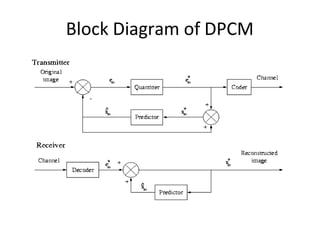
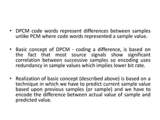
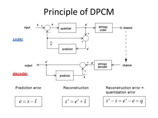
encode the difference between actual value of sample and
predicted value.

11. Principle of DPCM

12. Delta Modulation
• A Delta modulation (DM or Δ-modulation) is an analog-to-digital
and digital-to-analog signal conversion technique used for
transmission of voice information where quality is not of primary
importance.
• To achieve high signal-to-noise ratio, delta modulation must use
oversampling techniques, that is, the analog signal is sampled at a
rate several times higher than the Nyquist rate.
• Derived forms of delta modulation are continuously variable slope
delta modulation, delta-sigma modulation, and differential
modulation.
• Differential pulse-code modulation is the super-set of DM.

13. Features
• the analog signal is approximated with a series of
segments
• each segment of the approximated signal is compared to
the original analog wave to determine the increase or
decrease in relative amplitude
• the decision process for establishing the state of
successive bits is determined by this comparison
• only the change of information is sent, that is, only an
increase or decrease of the signal amplitude from the
previous sample is sent whereas a no-change condition
causes the modulated signal to remain at the same 0 or 1
state of the previous sample.

14. Principle of delta modulation

15. Differential Pulse Code Modulation
(DPCM)
• What if we look at sample differences, not the
samples themselves?
– dt = xt-xt-1
– Differences tend to be smaller
• Use 4 bits instead of 12, maybe?

16. Differential Pulse Code Modulation
(DPCM)
• Changes between adjacent samples small
• Send value, then relative changes
– value uses full bits, changes use fewer bits
– E.g., 220, 218, 221, 219, 220, 221, 222, 218,.. (all values between 218
and 222)
– Difference sequence sent: 220, +2, -3, 2, -1, -1, -1, +4....
– Result: originally for encoding sequence 0..255 numbers need 8 bits;
– Difference coding: need only 3 bits

17. Adaptive Differential Pulse Code
Modulation (ADPCM)
• Adaptive similar to DPCM, but adjusts the width of the
quantization steps
• Encode difference in 4 bits, but vary the mapping of bits to
difference dynamically
– If rapid change, use large differences
– If slow change, use small differences

18. Adaptive Delta Modulation (ADM)

19. A large step size is required when sampling those parts
of the input waveform of steep slope. But a large
step size worsens the granularity of the sampled
signal when the waveform being sampled is changing
slowly.
• A small step size is preferred in regions where the
message has a small slope. This suggests the
need for a controllable step size – the control
being sensitive to the slope of the sampled signal
• Hence ADM is prefered.

20. Adaptive Delta Modulation

21. VCA

22. Linear Predictive Coding (LPC)

23. Basic Concepts of LPC
• It is a parametric de-convolution algorithm
• x(n) is generated by an unknown sequence e(n)
exciting a unknown system V(Z) which is supposed to
be a linear non time-variant system.
• V(Z) = G(Z)/A(Z), E(Z)V(Z) = X(Z)
• G(Z) = Σj=0 gjZ , A(Z) = Σi=0 aiZ
Q -j P -i
• Where ai and gj are parameters, real and a0 = 1
• If an algorithm could estimate all these parameters,
then V(Z) could be found, and E(Z) could be found
also. This finishes de-convolution.

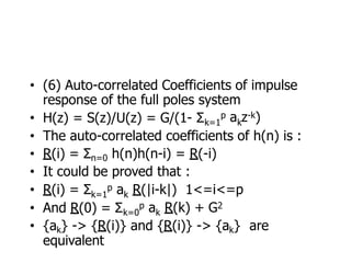
24. • There are some limitations for the model
• (1) G(Z) = 1 then V(Z) = 1/A(Z) this is so called “Full
Poles εodels” and the parametric de-convolution
became coefficients(ai) estimation problem.
• (2) e(n) sequence is of form Ge(n), where e(n) is a
periodic pulse or a Gaussian white noise sequence.
For the first case e(n) = Σ6(n-rNp) and for the second
case R(k) = E[e(n)e(n+k)] = 6(k) and the value of
e(n) satisfied with Normal distribution. G is a non-
negative real number controlling the amplitude.
• The way is x(n)->V(Z)(P,ai)->e(n),G->type of e(n)

25. • Suppose x(n) and type of e(n) are known, what is
the optimized estimation of P and ai, e(n) and G? It is
the LMS algorithm.
• Suppose x(n) is the predicted value of x(n), it is the
linear sum of previous P’ known values of x:
• x(n) = Σi=1
P’ ai x(n-i)
• The predicted error
• s(n) = x(n)-x(n) = x(n) - Σi=1
P’ ai x(n-i)
• It is a stochastic sequence. The variance of it could
be used to evaluate the quality of prediction.

26. • σ2 = Σnε2(n) (time average replaced means)
• It could be proved that if x(n) is generated by “full
poles” model : x(n) = -Σi=1
P ai x(n-i) + Ge(n) and
optimized P’ = P
, optimized ai = ai, σ2 is minimal.
• σ2 = Σn [x(n) -Σi=1
P ai x(n-i)]2
• ={Σn x2(n)}-2Σi=1
P ak{Σn x(n-k)x(n)}+
• Σk=1
PΣi=1
P akai{Σn x(n-k)x(n-i)}
• By setting ð(σ2 )/ ðak = 0 we can get
• -2 {Σn x(n-k)x(n)}+2Σi=1
P ai{Σn x(n-k)x(n-i)}=0
• Or Σi=1
P aiφ(k,i) = φ(k,0)
• if φ(k,i) =Σn x(n-k)x(n-i) 1<=i<=P and 1<=k<=P

27. i=1 i
• Σ P a φ(k,i) = φ(k,0), k=1~P is called δPC
canonical equations. There are some different
algorithms to deal with the solution.
k=0 k 0
• [σ2]min = Σ P a φ(k,0) with a = 1
• So if we have x(n), φ(k,i) could be calculated,
and equations could be solved to get ai and
[σ2]min also could be obtained. For short-time
speech signal according to different lower and
upper limitation of the summary we could
have different types of equations. We will
discuss these different algorithms later.

28. Auto-Correlated Solution of LPC
• Suppose windowed signal is xw(n)
• φ(k,i) = Σn xw(n-k)xw(n-i)
• If window length is N-1 then the summation
range will be 0~N+P-1
• φ(k,i) = Σm xw(m+(i-k))xw(m) = R(i-k) if n-i
= m
• φ(k,i) = R(i-k) = R(k-i) = R(|i-k|) <= R(0)
i=1 i
• The equations became Σ P a R(|i-k|)= - R(k)
1<=k<=P
• These are Toplitz equations and have high
efficient solution.

29. • |R(0) R(1) …… R(P-1)| |a1| | R(1) |
• |R(1) R(0) …… R(P-2)| |a2| | R(2) |
• |………………………………….| |...| = …...
• |R(P-1) R(P-2) … R(0) | |ap| | R(P) |
• 6.2.1 Durbin Algorithm
• 1. E(0) = R(0)
• 2. Ki = [ R(i) - Σ aj R(i-j)]/E
(i-1) (i-1)
• 3. ai = Ki
(i)
• 4. aj = aj – Kiai-j
(i) (i-1) (i-j)
• 5. E(i) = (1-Ki )E
2 (i-1)
• Final solution is aj = aj(p)
1<=i<=p
1<=j<=i-1
1<=j<=p

30. • For iteration i we got a set of
coefficients for the predictor of i-th
order and the minimal predicted error
energy E(i). We also can get it by {R(k)}
:
• E(i) = R(0) –Σk=1 akR(k), 1<=i<=p
i
• Ki is the reflect coefficient : -1<=Ki<=1
It is a sufficient and necessary condition
for stable H(z) during iteration.

31. • 6.2.2 Schur algorithm
• At first an auxilary sequence is defined. Its properties
are :
• (1) qi(j) = R(j) when i = 0
• (2) qi(j) = 0 when i > 0, j=1~p
• (3) qp(0) = E(p) is the predicted error energy.
• (4) |qi(j)| <= R(0), it is equal only if i=j=0
• The algorithm is as following:
• 1. r(j) = R(j)/R(0), r(-j) = r(j), j=0~p
• 2. a0 = 1, E(0) = 1
• 3. q0(j) = r(j) -p<j<p

32. • 4. i = 1, k1 = r(1)
• 5. For i-p<=j<=p
qi(j) = qi-1(j) + ki *qi-1 (i-j)
ki = qi-1(j)/qi(0)
aj = qi-1(i-j)
(i)
E(i) = E(i-1)(1-ki
• 6. If i<p, back to step 5
• 7. Stop
• If we only calculate ki, then only first two expressions
in step 5 are enough. It is suitable for fix-point
calculation (r<=1) or hardware implementation.

33. Covariance Solution of LPC
k=1~p, i=0~p
let n-i=m, m=-i~N-i-1
|φ(1,0)|
|φ(2,0)|
• If not using windowing, but limiting the range of
summation, we could get :
• σ2 = Σn=0
N-1ε2(n) n=0~N-1
• φ(k,i) = Σn=0
N-1 x(n-k)x(n-i)
• = Σm=-
N-i-1 x(m+(i-k))x(m)
i
• The equations will be like following :
• |φ(1,1) φ(1,2) …… φ(1,p)| |a1|
• |φ(2,1) φ(2,2) …… φ(2,p)| |a2|
• .………………………………………………=…………
• |φ(p,1) φ(p,2) …… φ(p,p)| |ap| |φ(p,0)|

34. Covariance Solution of LPC
• The matrix is a covariance matrix and it is positive
determined, but not Toplitz. There is no high efficient
algorithm to solve. Only common used LU algorithm
could be applied. Its advantage is not having big
predicted error on the two ends of window. So when
N~P the estimated parameters have more accuracy
than auto-correlated method. But in speech
processing very often N>>P, so the advantage is not
obvious.

35. LPC parameters and their relationships
1<=j<=p
1<=j<=i-1
at last aj= aj 1<=j<=p
(p)
• (1) Reflect Coefficients
• Also known as PARCOR coefficients
• If {aj} are known, ki could be found as following :
• aj = aj
(p)
• ki = ai(i)
• aj = (aj + aj ai-j )/(1-ki )
(i-1) (i) (i) (i) 2
• The inverse process :
• aj = ki
(i)
• aj = aj - kj ai-j
(i) (I-1) (i-1)
• -1<=ki<=1 is the sufficient and necessary condition
for stable system function

36. • (2) Coefficients of Logarithm Area Ratio
• gi = log(Ai+1/Ai) = log[(1-ki)/1+ki]) i=1~p
• Where A is the intersection area of i-th
segment of the lossless tube.
• ki = (1-exp(gi))/(1+exp(gi)) i=1~p
• (3) Cepstrum Coefficients
• cn = an + Σk=1 kckan-k/n, 1<=n<=p+1
n
•
n-1 kc a /n, n>p+1
= an + Σk=n-p k n-k

37. • (4) The Roots of Predictor
• A(z) = 1 – Σk=1 akz = Πk=1 (1-zk z ) = 0
p -k p -1
• Transfer to S-plane: zi = exp(siT)
• Suppose si = σi + jΩi , zi = zir + jzii , then
• Ωi = tan(zii/zir)/T andσi= log(zii
2 + zir )/(2T)
2
• (5)The impulse response of full poles system
• h(n) = Σk=1 akh(n-k)+σ(n) n>=0
p
• = 0 n<0
Σ

38. • (6) Auto-correlated Coefficients of impulse
response of the full poles system
• H(z) = S(z)/U(z) = G/(1- Σk=1 k
p a z-k)
• The auto-correlated coefficients of h(n) is :
• R(i) = Σn=0 h(n)h(n-i) = R(-i)
• It could be proved that :
k=1 k
• R(i) = Σ p a R(|i-k|) 1<=i<=p
• And R(0) = Σk=0 k
p a R(k) + G2
• {ak} -> {R(i)} and {R(i)} -> {ak} are
equivalent

39. • (7) Auto-correlated coefficients of impulse
response of the predicted error filter (inverse
filter)
• A(z) = 1 - Σ akz-k
• The impulse response is :
• a(n) = 6(n) - Σk=1
p ak6(n-k)
• = 1, n = 0; an , 0<n<=p; 0, otherwise
• Its auto-correlated function is :
• R(i) = Σk=1
p a(k)a(k+i) 0<=i<=p

40. • (8)Line Spectrum Pair (LSP) or Line
Spectrum Frequency (LSF)
• A(p)(z)=1-Σk=1 akz
p -k ( p is even)
• Define P(z) = A(p)(z)+z-(p+1)A(p)(z-1)
Q(z) = A(p)(z)- z-(p+1)A(p)(z-1)
• It could be proved that : All roots of P(z) and
Q(z) are on the unit circle and alternatively
arranged on it provided the roots of A(z) are
inside the unit circle.

41. • Replace z with expjω:
• P(expjω)=|A(P)(expjω)|expjφ(ω)[1+exp[-j((p+1)ω+
2φ(ω))]
• Q(expjω)=|A(P)(expjω)|expjφ(ω)[1+exp[-j((p+1)ω+
2φ(ω)+π)]
• If the roots of A(P)(z) are inside the unit circle, whenωis
0~π, φ(ω) changes from 0 and returns to 0, the amount
[(p+1)ω+2φ(ω)] will be 0~(p+1)π
• P(expjω)=0 : [(p+1)ω+2φ(ω)]=kπ, k=1,3,…P+1
• Q(expjω)=0 : [(p+1)ω+2φ(ω)]=kπ, k=0,2,…P
• The roots of P and Q : Zk = expjωk [(p+1)ω+2φ(ω)]=kπ,
k=0,1,2,…P+1
• And ω0 < ω1 < ω2 < … < ωP < ωP+1

42. • If a1 ~ap are known, LSP could be found by
(p) (p)
A(z) -> P(z) -> p(w) -> f1, f2, … fp
• If f1~fp are known, ai
(p) could be found by P(z)
1 p
and Q(z) -> A(z) = P(z) + Q(z) -> a (p)~a (p)

43. Thank you