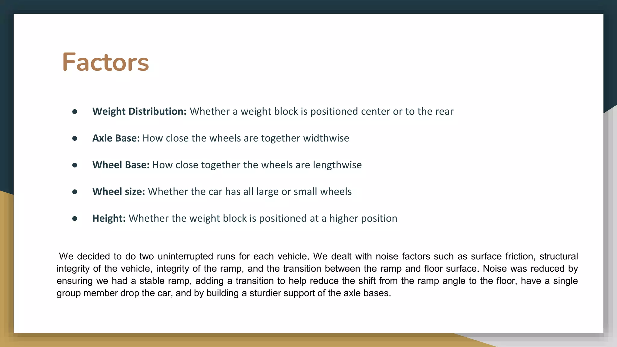
The document describes a design of experiments project to optimize factors that affect the distance traveled by a LEGO car down a ramp. Key factors tested were wheel base, axle base, wheel size, height, and weight distribution. ANOVA analysis identified significant main effects and interactions. The optimal design was found to be large wheel base, small axle base, large wheel size, and large height. This car provided the best performance at a reasonable cost. Recommendations included focusing on wheel base and size for performance while keeping other factors small to control costs without compromising effectiveness.

1. LEGO PROJECT
SCM517 Group
Fall 2022

2. Contents
1) Objective & Factors
2) Response Variables & Experimental setup
3) DOE & Analysis
4) Recommendations & Conclusion

3. Objective
“To create a car that travels the most
distance at a minimal cost with the
materials and constraints provided”

4. Factors
● Weight Distribution: Whether a weight block is positioned center or to the rear
● Axle Base: How close the wheels are together widthwise
● Wheel Base: How close together the wheels are lengthwise
● Wheel size: Whether the car has all large or small wheels
● Height: Whether the weight block is positioned at a higher position
We decided to do two uninterrupted runs for each vehicle. We dealt with noise factors such as surface friction, structural
integrity of the vehicle, integrity of the ramp, and the transition between the ramp and floor surface. Noise was reduced by
ensuring we had a stable ramp, adding a transition to help reduce the shift from the ramp angle to the floor, have a single
group member drop the car, and by building a sturdier support of the axle bases.

5. Response Variable
● y: Distance travelled by the car down the ramp
● Units: centimeters(cm)

6. Level of factors
Factor (X) Low(-) High(+)
Wheel Base 6.5 cm 11.3 cm
Axle Base 1.6 cm 6.48 cm
Wheel size Small Large
Height 5.3 cm 7.5 cm
Weight Distribution Back Center
Wheel Base
Axle Base
Wheel size
*center
Weight Distribution
Height

7. Experimental Setup
● Equipment used: Block of books, Cardboard,
Measuring tape
● Height of the block of books: 31 cm
● Length of the ramp: 76 cm
● Width of the ramp: 50.5 cm
● Angle at which the ramp was placed: 30ᵒ

8. Design Of Experiments
1) Factorial Design
2) Preliminary model (ANOVA, Plot Analysis)
3) Model Refinement (ANOVA, Plot Analysis)
4) Interpret results

9. 1) Factorial Design
- 5 factors:
- Two levels for each factor
- Wheel base: 6.5 and 11.3cm
- Axle base: 1.6 and 6.48 cm
- Height: Small and Large
- Wheel size: Small and Large
- Weight distribution: Back and Center
- 2 replications
- Response variable: Travel distance from the
ramp
- Goal: Maximize the travel distance

10. 2) Preliminary model (ANOVA)
- The Anova analysis highlights the
insignificant factors and interactions.
- These factors would have insignificant effect
on response so analysis would be performed
on significant factor.

11. 2) Preliminary model (ANOVA)
y = 113.188
+ 5.312 Wheel Base - 0.469 Axle Base + 6.906 Wheel size - 0.469 Height
+ 0.219 Weight Dist - 2.156 Wheel Base*Axle Base - 0.531 Wheel Base*Wheel size
+ 2.844 Wheel Base*Height - 1.531 Wheel Base*Weight Dist - 0.562 Axle Base*Wheel
size
- 1.812 Axle Base*Height - 1.312 Axle Base*Weight Dist + 2.625 Wheel size*Height
- 2.312 Wheel size*Weight Dist + 2.312 Height*Weight Dist
- 0.313 Wheel Base*Axle Base*Wheel size - 0.813 Wheel Base*Axle Base*Height
+ 1.875 Wheel Base*Axle Base*Weight Dist - 0.500 Wheel Base*Wheel size*Height
+ 1.375 Wheel Base*Wheel size*Weight Dist - 2.125 Wheel Base*Height*Weight Dist
+ 0.594 Axle Base*Wheel size*Height + 2.469 Axle Base*Wheel size*Weight Dist
- 2.031 Axle Base*Height*Weight Dist - 0.719 Wheel size*Height*Weight Dist
- 1.094 Wheel Base*Axle Base*Wheel size*Height
- 2.656 Wheel Base*Axle Base*Wheel size*Weight Dist
+ 2.969 Wheel Base*Axle Base*Height*Weight Dist
+ 1.406 Wheel Base*Wheel size*Height*Weight Dist
+ 1.625 Axle Base*Wheel size*Height*Weight Dist
- 1.312 Wheel Base*Axle Base*Wheel size*Height*Weight Dist
Regression Equation in Uncoded Units

12. 2) Preliminary model (Normal Plot)
- From the Normal Probability Plot
and Pareto Chart, we can find which
model is significant
- Significant factors:
- C, A, ABDE, AD, CD, BCE, DE, ABE,
CDE, ACE, AE, BD, BDE, ADE, AB, CE,
ABCE
- Non-Significant factors:
- ABCDE, BE, ABCD, ABD, CDE, BCD, BC,
AC, ACD, D, B, ABC
➢ Select Significant Effects and make
another Factorial Model (Model
Refinement)

13. 2) Preliminary model (Residual)
- Normality test looks pretty good and data
distributed along the line
- Residual vs fits plot depicts equal variance in
data but there is pattern seen in the Versus
Fits plot
- Residual vs Order plot doesn’t present any
cycle/trends which implies less uncontrolled
variable impact on experiment
*Outliers:

14. 2) Plot Analysis (Main Effects & Interaction)
- Higher Wheel base implies higher speed
- Lower Axle base implies higher speed
- Higher Wheel size implies higher speed
- Higher Height implies lower speed
- Weight distribution doesn’t impact speed much
- Interaction plot shows positive
interaction Wheel size and
Wheel base.
- Contour plot has higher area
coverage for Wheel size and
Wheel base and pimples same
as interaction plot.

15. 3) Model Refinement (ANOVA)
- Refined model has increase in R-sq(pred)
which implies better predictions.
- All main effects and interactions are
significant with P-value <= 0.05

16. 3) Model Refinement (ANOVA)
y = 113.188 + 5.312 Wheel Base + 6.906 Wheel size - 2.156 Wheel Base*Axle Base
+ 2.844 Wheel Base*Height - 1.531 Wheel Base*Weight Dist - 1.813 Axle
Base*Height
+ 2.625 Wheel size*Height - 2.313 Wheel size*Weight Dist + 2.312 Height*Weight
Dist
+ 1.875 Wheel Base*Axle Base*Weight Dist + 1.375 Wheel Base*Wheel size*Weight
Dist
- 2.125 Wheel Base*Height*Weight Dist + 2.469 Axle Base*Wheel size*Weight Dist
- 2.031 Axle Base*Height*Weight Dist - 2.656 Wheel Base*Axle Base*Wheel
size*Weight Dist
+ 2.969 Wheel Base*Axle Base*Height*Weight Dist
+ 1.406 Wheel Base*Wheel size*Height*Weight Dist
+ 1.625 Axle Base*Wheel size*Height*Weight Dist
Regression Equation in Coded Units.

17. 3) Plot Analysis (Residual)
- Normality test looks pretty good and data is
distributed along the line.
- Residual vs fits plot depicts equal variance in data
and model fit is adequate.
- Residual vs Order plot doesn’t present any
cycle/trends which implies less uncontrolled
variable impact on experiment.
*Outliers:

18. 3) Plot Analysis (Main Effects & Interaction)
- ‘Wheel Size’ is the most important factor in this experiment.
- High ‘Wheel Base’ and High ‘Wheel Size’ will give the best
performance for the car.
- Impact of ‘Wheel Size’ is bigger than ‘Wheel Base’

19. Cost Analysis
- Calculate the cost of each model using formula as below
Model cost = Basic Model Cost ($19,600)
+ Axle Base ($3,000 or $6,000)
+ Wheel Size ($2,000 or $4,000)
+ Height ($0 or $3,000)
● The most effective car had a cost of $29,600.
● The most ineffective car cost $27,600, which was also the most cost inefficient at $208 per inch traveled.
● The most efficient car also happened to be the most effective car in the experiment at $106 per inch.

20. Cost Analysis
Best Performing Models
& Cost Effective
Worst Models - According to the cost analysis,
one should spend the right
amount of money to get into
larger wheels than wasting it in
other areas.

21. Types of cars:
Base Model
Most Expensive Model
Most Economical Model
Worst Performing Model
Best Performing Model

22. Recommendations & Conclusion
<Recommendations>
➔ Based on Analysis and experimental results, our recommendation for best performing car is using Large wheel
base and Large wheel size together and the most economic car is using small axle base & small wheel size & low
height.
➔ ‘Wheel base’ and ‘Wheel size’ contributed the most to the best performance of our model, those two level of
factors should be in default. And then we’d recommend add another factors to develop and achieve better
performance.
➔ The most important factors are ‘Wheel Size’ and ‘Wheel base’. So if we consider the cost, maintain low height
and a smaller axel base would keep the cost factor low without majorly compromising the performance.
<Conclusion>
Ideal Car : Large wheel base, Small axle base, Large wheel size, Large height, and Rear weight distribution
➔ Environment in which the experiment was conducted, was not changed - to avoid noise
➔ A cardboard was used to give the car a smooth transition from the ramp to the ground

23. Thank You