Lecture19:PHY 712 Electrodynamics-waveguides

PHY 712 Spring 2019 -- Lecture 19 1
02/27/2019
PHY 712 Electrodynamics
9-9:50 AM Olin 105
Plan for Lecture 19:
Chap. 8 in Jackson – Wave Guides
1. TEM, TE, and TM modes
2. Justification for boundary conditions;
behavior of waves near conducting
surfaces

02/27/2019
4 PM in Olin 101

02/27/2019

02/27/2019
For linear isotropic media and no sources: ;
Coulomb's law: 0
Ampere-Maxwell's law: 0
Faraday's law: 0
No magnetic monopoles:
t
t
 

 
 

  


  

D E B H
E
E
B
B
E
0
 
B
Maxwell’s equations

02/27/2019
 
0
2
2
2
2


























t
t
t
B
B
E
B
E
B



Analysis of Maxwell’s equations without sources -- continued:
0
:
monopoles
magnetic
No
0
:
law
s
Faraday'
0
:
law
s
Maxwell'
-
Ampere
0
:
law
s
Coulomb'


















B
B
E
E
B
E
t
t

 
0
2
2
2
2


























t
t
t
E
E
B
E
B
E


02/27/2019
2
2
0
0
2
2
2
2
2
2
2
2
2
2
where
0
1
0
1
n
c
c
v
t
v
t
v















E
E
B
B
Both E and B fields are solutions to a wave equation:
       
t
i
i
t
i
i
e
t
e
t 
 






 r
k
r
k
E
r
E
B
r
B 0
0 ,
,
:
equation
wave
to
solutions
wave
Plane

02/27/2019
       
0
0
2
2
2
0
0
where
,
,
:
equation
wave
to
solutions
wave
Plane

























 



n
c
n
v
e
t
e
t t
i
i
t
i
i
k
E
r
E
B
r
B r
k
r
k
Note: e, m, n, k can all be complex; for the moment we will
assume that they are all real (no dissipation).
0
ˆ
and
0
ˆ
:
note
also
ˆ
0
:
law
s
Faraday'
from
t;
independen
not
are
and
that
Note
0
0
0
0
0
0
0















B
k
E
k
E
k
E
k
B
B
E
B
E
c
n
t

For real
e, m, n, k

02/27/2019
     
0
ˆ
and
where
,
ˆ
,
:
waves
netic
electromag
plane
of
Summary
0
0
0
2
2
2
0
0


























 

 



E
k
k
E
r
E
E
k
r
B r
k
r
k







n
c
n
v
e
t
e
c
n
t t
i
i
t
i
i
2
2
0
0
2
0
Poynting vector and energy density:
1
ˆ ˆ
2 2
1
2
avg
avg
n
c
u

 

 

E
S k E k
E
E0
B0
k

02/27/2019
Transverse electric and magnetic waves (TEM)
     
0
0
2 2
2
0
0 0
ˆ
, ,
ˆ
where and 0
i i t i i t
n
t e t e
c
n
n
v c
 
  
 
   
 

 
 
 
   
    
   
   
k r k r
k E
B r E r E
k k E
E0
B0
k
TEM modes describe
electromagnetic waves in lossless
media and vacuum
For real
e, m, n, k

02/27/2019
Effects of complex dielectric; fields near the surface on an
ideal conductor
     
   
 
t
i
c
in
I
R
t
i
i
b
b
b
R
e
e
t
c
in
n
e
t
t
t
t
t



 

























































r
k
r
k
r
k
E
r
E
k
k
E
r
E
E
H
E
F
F
E
E
H
H
E
H
E
E
H
E
J
E
D
ˆ
/
0
/
ˆ
0
2
2
2
,
ˆ
re
whe
,
:
for
form
wave
Plane
,
0
0
0
:
and
of
in terms
equations
s
Maxwell'
:
medium
isotropic
an
for
Suppose

02/27/2019
     
 
2
2 2
0
2
2
2
Plane wave form for :
ˆ
, where
0
0
i i t
R I
b
R I b
t e n in
c
t t
c
n in i c
 
 




 
  
 
 
   
 
 
 
    
k r
E
E r E k k
E
Some details:

02/27/2019
Fields near the surface on an ideal conductor -- continued
















1
2
1
For
1
1
2
1
1
2
:
system
our
For
2
/
1
2
2
/
1
2














































I
R
b
b
I
b
b
R
n
c
n
c
n
c
n
c
   
     
ˆ ˆ
/ /
0
,
1
ˆ ˆ
, , ,
i i t
t e e
n i
t t t
c
  
 
   
  

    
k r k r
E r E
H r k E r k E r

02/27/2019
Some representative values of skin depth
Ref: Lorrain2
and Corson
s (107
S/m) m/m0
d (0.001m)
at 60 Hz
d (0.001m)
at 1 MHz
Al 3.54 1 10.9 84.6
Cu 5.80 1 8.5 66.1
Fe 1.00 100 1.0 10.0
Mumetal 0.16 2000 0.4 3.0
Zn 1.86 1 15.1 117
1
2
R I
n n
c c
  

  

02/27/2019
Relative energies associated with field
2
2
2 2 2
2 2
Electric energy density:
Magnetic energy density:
Ratio inside conducting media:
2
1
b
b b b
i


    



 

E
H
E
H
2
2
2
0 0
2
2
2
0
2
0
=2
For 1 magnetic energy dominates
Note that in free space, 1
b
b
  

  






E
H
E
H


02/27/2019
 
i
c
in
n
c
n
c
n
c
I
R
I
R









1
1
limit,
In this
1
2
1
For
0
0 











   
     
ˆ ˆ
/ /
0
,
1
ˆ ˆ
, , ,
i i t
t e e
n i
t t t
c
  
 
   
 

   
k r k r
E r E
H r k E r k E r
z
r||
0

02/27/2019
   
     
ˆ ˆ
/ /
0
,
1
ˆ ˆ
, , ,
i i t
t e e
n i
t t t
c
  
 
   
 

   
k r k r
E r E
H r k E r k E r
z
r||
0
   
   
ˆ ˆ
/ /
0
Note that the field is larger than field so we can write:
,
1 ˆ
, ,
2
i i t
t e e
i
t t
  

   
 

 
k r k r
H E
H r H
E r k H r

Boundary values for ideal conductor
At the boundary of an
ideal conductor, the E
and H fields decay in the
direction normal to the
interface.
   
   
t
i
t
e
e
t t
i
i
,
ˆ
2
1
,
,
:
conductor
the
Inside
/
ˆ
0
/
ˆ
r
H
k
r
E
H
r
H r
k
r
k




 







k̂
H0
n̂
 
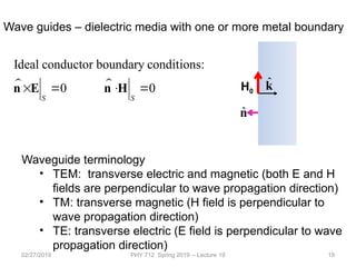
Ideal conductor boundary condit
0 0
ions:
S S
   
n E n H
02/27/2019

Waveguide terminology
• TEM: transverse electric and magnetic (both E and H
fields are perpendicular to wave propagation direction)
• TM: transverse magnetic (H field is perpendicular to
wave propagation direction)
• TE: transverse electric (E field is perpendicular to wave
propagation direction)
02/27/2019
Wave guides – dielectric media with one or more metal boundary
k̂
H0
n̂
 
Ideal conductor boundary condit
0 0
ions:
S S
   
n E n H

Analysis of rectangular waveguide
Boundary conditions at surface of waveguide:
Etangential=0, Bnormal=0
z
x
y
Cross section view b
a
02/27/2019

Analysis of rectangular waveguide
z
x
y
     
 
 
     
 
 
t
i
ikz
z
y
x
t
i
ikz
z
y
x
e
y
x
E
y
x
E
y
x
E
e
y
x
B
y
x
B
y
x
B












z
y
x
E
z
y
x
B
ˆ
,
ˆ
,
ˆ
,
ˆ
,
ˆ
,
ˆ
,
02/27/2019
Inside the dielectric medium: (assume to be real)
0 0
=0 0
t t


   
 
    
 
E B
B E
E B

Solution of Maxwell’s equations within the pipe:
2 2
2 2
2 2
Combining Faraday's Law and Ampere's Law, we find that each field
component must satisfy a two-dimensional Helmholz equation:
( , ) 0.
x
k
x y
E x y

 
 
   
 




02/27/2019
0
2 2
2 2 2
For the rectangular wave guide discussed in Section 8.4 of your
text a solution for a TE mode can hav
( , ) 0 and ( , ) cos cos ,
wit
e:
h
z z
mn
m x n y
E x y B x y B
a b
m n
k k
a b
 
 

   
     
   
 
   
   
 
   
   
 
 

Maxwell’s equations within the pipe in terms of all 6 components:
0.
0.
y
x
z
y
x
z
B
B
ikB
x y
E
E
ikE
x y


  
 


  
 
.
.
.
z
y x
z
x y
y x
z
E
ikE i B
y
E
ikE i B
x
E E
i B
x y




 


 

 
 
 
.
.
.
z
y x
z
x y
y x
z
B
ikB i E
y
B
ikB i E
x
B B
i E
x y




 


 

 
 
 
02/27/2019
For TE mode with 0
z
x y
y x
E
k
B E
k
B E






TE modes for rectangular wave guide continued:
0
0
2 2 2 2
0
2 2 2 2
( , ) 0 and ( , ) cos cos ,
cos sin ,
sin
z z
z
x y
z
y x
m x n y
E x y B x y B
a b
B
i i n m x n y
E B B
k k y b a b
m n
a b
B
i i m
E B B
k k x a
m n
a b
 
     
  
   
  
   
     
   

     
      
       
   

 
   
   
 
 

  
   
   

 
   
   
 
 
cos .
m x n y
a b
 
   
   
   
tangential
normal
0 because: ( ,0) ( , ) 0
and
Check boundary conditions:
(0, ) ( , ) 0
0
.
x x
y y
E x E x b
E y E a y
 
  

E
B
02/27/2019

Solution for m=n=1
 
 
   
 
   


























































b
y
n
a
x
m
a
m
B
y
x
iE
b
y
n
a
x
m
b
n
B
y
x
iE
b
y
n
a
x
m
B
y
x
B
b
n
a
m
y
b
n
a
m
x
z














cos
sin
/
,
sin
cos
/
,
cos
cos
,
2
2
0
2
2
0
0
 
y
x
Bz ,
 
y
x
iEx ,
 
y
x
iEy ,
02/27/2019

Solution for m=n=1
2 2
2 2 2
mn
m n
k k
a b
 

 
   
   
 
   
   
 
 
k
w
02/27/2019

     
 
 
     
 
 
         
         
d
p
k
kz
y
x
B
kz
y
x
B
z
y
x
B
kz
y
x
E
kz
y
x
E
z
y
x
E
e
z
y
x
E
z
y
x
E
z
y
x
E
e
z
y
x
B
z
y
x
B
z
y
x
B
i
i
i
i
i
i
t
i
z
y
x
t
i
z
y
x

















cos
,
or
sin
,
,
,
cos
,
or
sin
,
,
,
:
general
In
ˆ
,
,
ˆ
,
,
ˆ
,
,
ˆ
,
,
ˆ
,
,
ˆ
,
,
z
y
x
E
z
y
x
B
27
Resonant cavity
z
x
y
d
z
b
y
a
x






0
0
0
02/27/2019

02/27/2019
Resonant cavity
z
x
y
d
z
b
y
a
x






0
0
0




















































2
2
2
2
2
2
2
2
2
1
d
p
b
n
a
m
b
n
a
m
d
p
k










k
02/27/2019
Wave guides – dielectric media with one or more metal boundary
Coaxial cable
TEM modes
Simple optical pipe
TE or TM modes
Waveguide terminology
• TEM: transverse electric and magnetic (both E and H
fields are perpendicular to wave propagation direction)
• TM: transverse magnetic (H field is perpendicular to
wave propagation direction)
• TE: transverse electric (E field is perpendicular to wave
propagation direction)
E
H
k

Wave guides
Coaxial cable
TEM modes
Top view:
a
b
m e
z
0
0
for
:
medium
inside
equations
s
Maxwell'















B
E
B
E
B
E
ε
iω
i
b
a



(following problem 8.2 in
Jackson’s text)
Inside medium,
m e assumed to
be real
02/27/2019

Electromagnetic waves in a coaxial cable -- continued
ˆ
cos
ˆ
sin
ˆ
ˆ
sin
ˆ
cos
ˆ
ˆ
ˆ
for
solution
Example
0
0
y
x
φ
y
x
ρ
φ
B
ρ
E






































t
i
ikz
t
i
ikz
e
a
B
e
a
E
b
a
Top view:
a
b
m e
r
f
  z
B
E
S ˆ
2
2
1
:
)
,
(with
medium
cable
thin
vector wi
Poynting
2
2
0
*


















a
B
avg



0
0
:
Find
B
E
k


02/27/2019

Electromagnetic waves in a coaxial cable -- continued
Top view:
a
b
m e
r
f
  







  a
b
a
B
d
d avg
b
a
ln
ˆ
:
material
cable
in
power
averaged
Time
2
2
0
2
0 






z
S
02/27/2019

Lecture19:PHY 712 Electrodynamics-waveguides

More Related Content

Similar to Lecture19:PHY 712 Electrodynamics-waveguides

Recently uploaded

Lecture19:PHY 712 Electrodynamics-waveguides