This document provides an overview of text classification and the Naive Bayes algorithm for text classification. It begins by defining text classification and giving examples like spam filtering and document classification. It then explains supervised classification and the goal of learning a classifier from labeled training data. The document spends several slides explaining the Naive Bayes algorithm for text classification, including the Naive Bayes assumption of conditional independence between features. It discusses parameter estimation and smoothing techniques to avoid overfitting. Finally, it compares the multivariate Bernoulli and multinomial Naive Bayes models for text classification.

1. Text Classification
1
Lecture 15: Classification
Web Search and Mining

2. Text Classification
2
Relevance feedback revisited
 In relevance feedback, the user marks a few
documents as relevant/nonrelevant
 The choices can be viewed as classes or categories
 For several documents, the user decides which of
these two classes is correct
 The IR system then uses these judgments to build a
better model of the information need
 So, relevance feedback can be viewed as a form of
text classification (deciding between several classes)
 The notion of classification is very general and has
many applications within and beyond IR
Classification Problem

3. Text Classification
3
Spam filtering: Another text
classification task
From: "" <takworlld@hotmail.com>
Subject: real estate is the only way... gem oalvgkay
Anyone can buy real estate with no money down
Stop paying rent TODAY !
There is no need to spend hundreds or even thousands for similar courses
I am 22 years old and I have already purchased 6 properties using the
methods outlined in this truly INCREDIBLE ebook.
Change your life NOW !
=================================================
Click Below to order:
http://www.wholesaledaily.com/sales/nmd.htm
=================================================
Classification Problem

4. Text Classification
4
Text classification
 Introduction to text classification
 Also widely known as “text categorization”. Same thing.
 Machine learning based text classification methods
 Naïve Bayes
 Including a little on Probabilistic Language Models
 Rocchio method
 kNN
 Support vector machine (SVM)
Classification Problem

5. Text Classification
5
Supervised Classification
 Given:
 A description of an instance, d  X
 X is the instance language or instance space.
 A fixed set of classes:
C = {c1, c2,…, cJ}
 A training set D of labeled documents with each labeled
document ⟨d,c⟩∈X×C
 Determine:
 A learning method or algorithm which will enable us to
learn a classifier γ:X→C
 For a test document d, we assign it the class γ(d) ∈ C
Classification Problem

6. Text Classification
6
Multimedia GUI
Garb.Coll.
Semantics
ML Planning
planning
temporal
reasoning
plan
language...
programming
semantics
language
proof...
learning
intelligence
algorithm
reinforcement
network...
garbage
collection
memory
optimization
region...
“planning
language
proof
intelligence”
Training
Data:
Test
Data:
Classes:
(AI)
Document Classification
(Programming) (HCI)
... ...
(Note: in real life there is often a hierarchy, not present in
the above problem statement; and also, you get papers on
ML approaches to Garb. Coll.)
Classification Problem

7. Text Classification
7
More Text Classification Examples
Many search engine functionalities use classification
 Assigning labels to documents or web-pages:
 Labels are most often topics such as Yahoo-categories
 "finance," "sports," "news>world>asia>business"
 Labels may be genres
 "editorials" "movie-reviews" "news”
 Labels may be opinion on a person/product
 “like”, “hate”, “neutral”
 Labels may be domain-specific
 "interesting-to-me" : "not-interesting-to-me”
 “contains adult language” : “doesn’t”
 language identification: English, French, Chinese, …
 search vertical: about Linux versus not
 “link spam” : “not link spam”
Classification Problem

8. Text Classification
8
Naïve Bayes methods

9. Text Classification
9
Probabilistic relevance feedback
 Rather than reweighting in a vector space…
 If user has told us some relevant and some irrelevant
documents, then we can proceed to build a
probabilistic classifier,
 such as the Naive Bayes model we will look at today:
 P(tk|R) = |Drk| / |Dr|
 P(tk|NR) = |Dnrk| / |Dnr|
 tk is a term; Dr is the set of known relevant documents; Drk is the
subset that contain tk; Dnr is the set of known irrelevant
documents; Dnrk is the subset that contain tk.
Naïve Bayes

10. Text Classification
10
Bayesian Methods
 Learning and classification methods based on
probability theory.
 Bayes theorem plays a critical role in probabilistic
learning and classification.
 Builds a generative model that approximates how
data is produced
 Uses prior probability of each category given no
information about an item.
 Categorization produces a posterior probability
distribution over the possible categories given a
description of an item.
Naïve Bayes

11. Text Classification
11
Bayes’ Rule for text classification
 For a document d and a class c

P(c,d)  P(c | d)P(d)  P(d |c)P(c)
P(c | d) 
P(d |c)P(c)
P(d)
Naïve Bayes

12. Text Classification
12
Naive Bayes Classifiers
Task: Classify a new instance d based on a tuple of attribute values
into one of the classes cj  C

 n
x
x
x
d ,
,
, 2
1 
)
,
,
,
|
(
argmax 2
1 n
j
C
c
MAP x
x
x
c
P
c
j



)
,
,
,
(
)
(
)
|
,
,
,
(
argmax
2
1
2
1
n
j
j
n
C
c x
x
x
P
c
P
c
x
x
x
P
j 



)
(
)
|
,
,
,
(
argmax 2
1 j
j
n
C
c
c
P
c
x
x
x
P
j



MAP is “maximum a posteriori” = most likely class
Naïve Bayes

13. Text Classification
13
Naïve Bayes Classifier:
Naïve Bayes Assumption
 P(cj)
 Can be estimated from the frequency of classes in the
training examples.
 P(x1,x2,…,xn|cj)
 O(|X|n•|C|) parameters
 Could only be estimated if a very, very large number of
training examples was available.
Naïve Bayes Conditional Independence Assumption:
 Assume that the probability of observing the conjunction of
attributes is equal to the product of the individual
probabilities P(xi|cj).
Naïve Bayes

14. Text Classification
14
Flu
X1 X2 X5
X3 X4
fever
sinus cough
runnynose muscle-ache
The Naïve Bayes Classifier
 Conditional Independence Assumption:
features detect term presence and are
independent of each other given the class:
)
|
(
)
|
(
)
|
(
)
|
,
,
( 5
2
1
5
1 C
X
P
C
X
P
C
X
P
C
X
X
P 


 

Naïve Bayes

15. Text Classification
15
Learning the Model
 First attempt: maximum likelihood estimates
 simply use the frequencies in the data
)
(
)
,
(
)
|
(
ˆ
j
j
i
i
j
i
c
C
N
c
C
x
X
N
c
x
P




C
X1 X2 X5
X3 X4 X6
N
c
C
N
c
P
j
j
)
(
)
(
ˆ 

Naïve Bayes

16. Text Classification
16
Problem with Maximum Likelihood
 What if we have seen no training documents with the word muscle-
ache and classified in the topic Flu?
 Zero probabilities cannot be conditioned away, no matter the other
evidence!
0
)
(
)
,
(
)
|
(
ˆ 5
5 






f
C
N
f
C
t
X
N
f
C
t
X
P

 i i
c c
x
P
c
P )
|
(
ˆ
)
(
ˆ
max
arg

Flu
X1 X2 X5
X3 X4
fever
sinus cough
runnynose muscle-ache
)
|
(
)
|
(
)
|
(
)
|
,
,
( 5
2
1
5
1 C
X
P
C
X
P
C
X
P
C
X
X
P 


 

Naïve Bayes
Multivariate
Bernoulli
Model

17. Text Classification
17
Smoothing to Avoid Overfitting
k
c
C
N
c
C
x
X
N
c
x
P
j
j
i
i
j
i






)
(
1
)
,
(
)
|
(
ˆ
 Somewhat more subtle version
# of values of Xi
m
c
C
N
mp
c
C
x
X
N
c
x
P
j
k
i
j
k
i
i
j
k
i






)
(
)
,
(
)
|
(
ˆ ,
,
,
overall fraction in
data where Xi=xi,k
extent of
“smoothing”
Naïve Bayes

18. Text Classification
18
Naïve Bayes via a class conditional
language model = multinomial NB
 Effectively, the probability of each class is done as
a class-specific unigram language model
C
w1 w2 w3 w4 w5 w6
Naïve Bayes

19. Text Classification
19
Using Multinomial Naive Bayes Classifiers to
Classify Text: Basic method
 Attributes are text positions, values are words.
 Still too many possibilities
 Assume that classification is independent of the positions
of the words
 Use same parameters for each position
 Result is bag-of-words model (over tokens not types)
)
|
text"
"
(
)
|
our"
"
(
)
(
argmax
)
|
(
)
(
argmax
1
j
j
j
n
j
j
C
c
i
j
i
j
C
c
NB
c
x
P
c
x
P
c
P
c
x
P
c
P
c








Naïve Bayes

20. Text Classification
20
 Textj  single document containing all docsj
 for each word xk in Vocabulary
 njk  number of occurrences of xk in Textj
 nj number of words in Textj

Naive Bayes: Learning
Running example: document classification
 From training corpus, extract Vocabulary
 Calculate required P(cj) and P(xk | cj) terms
 For each cj in C do
 docsj  subset of documents for which the target class is cj

|
|
1
)
|
(
Vocabulary
n
n
c
x
P
j
jk
j
k



|
documents
#
total
|
|
|
)
(
j
j
docs
c
P 
Naïve Bayes

21. Text Classification
21
Naive Bayes: Classifying
 positions  all word positions in current document
which contain tokens found in Vocabulary
 Return cNB, where




positions
i
j
i
j
C
c
NB c
x
P
c
P
c )
|
(
)
(
argmax
j
Naïve Bayes

22. Text Classification
22
Naive Bayes: Time Complexity
 Training Time: O(|D|Lave + |C||V|))
where Lave is the average length of a document in D.
 Assumes all counts are pre-computed in O(|D|Lave) time during one
pass through all of the data.
 Generally just O(|D|Lave) since usually |C||V| < |D|Lave
 Test Time: O(|C| Lt)
where Lt is the average length of a test document.
 Very efficient overall, linearly proportional to the time needed to
just read in all the data.
Why?
Naïve Bayes

23. Text Classification
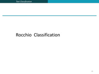
23
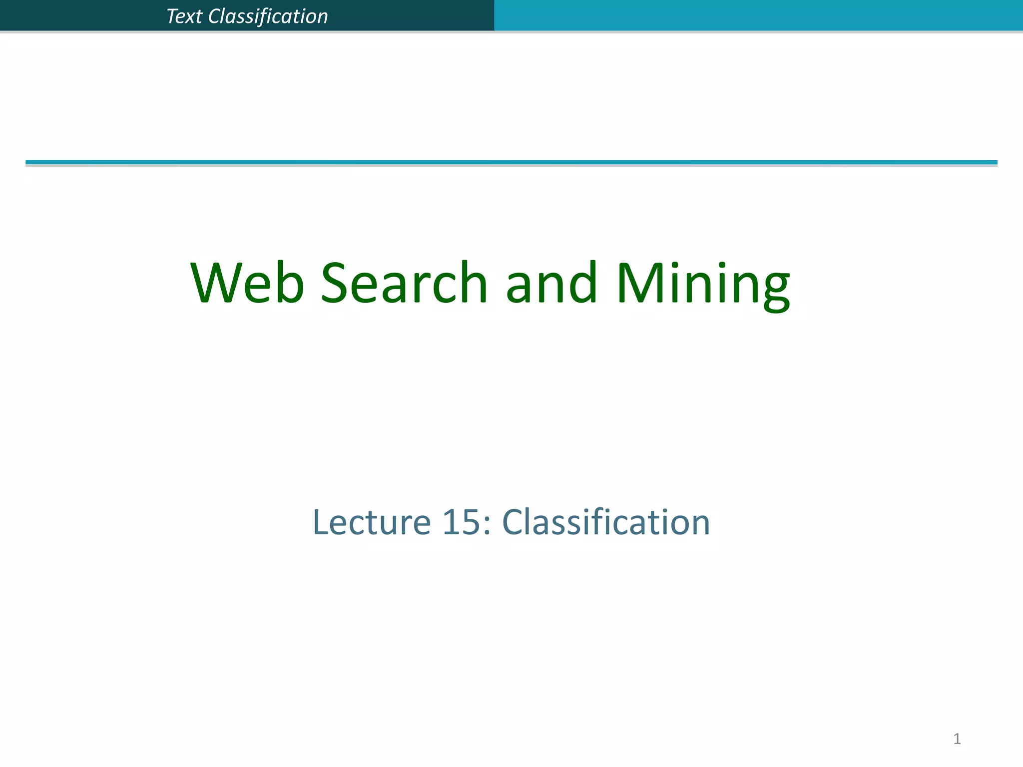
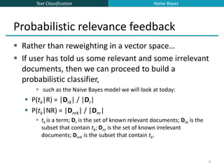
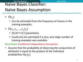
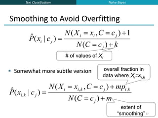
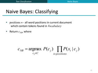
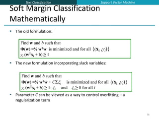
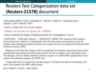
Underflow Prevention: using logs
 Multiplying lots of probabilities, which are between 0 and 1
by definition, can result in floating-point underflow.
 Since log(xy) = log(x) + log(y), it is better to perform all
computations by summing logs of probabilities rather than
multiplying probabilities.
 Class with highest final un-normalized log probability score is
still the most probable.
 Note that model is now just max of sum of weights…
cNB  argmax
cj C
[log P(c j )  log P(xi |c j )
ipositions
 ]
Naïve Bayes

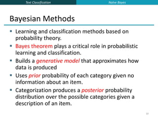
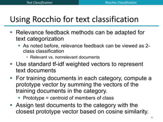
24. Text Classification
24
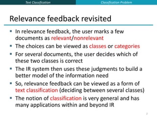
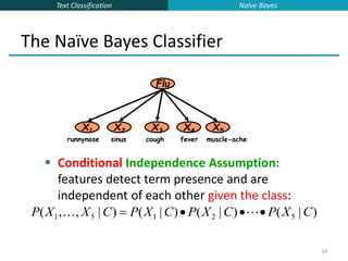
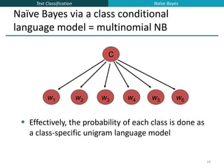
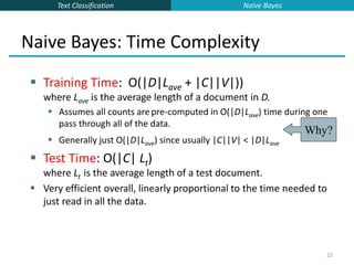
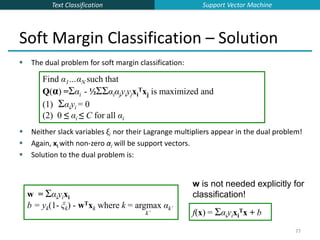
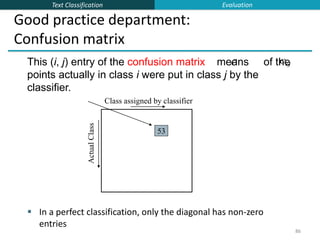
Naive Bayes Classifier
 Simple interpretation: Each conditional parameter
log P(xi|cj) is a weight that indicates how good an
indicator xi is for cj.
 The prior log P(cj) is a weight that indicates the
relative frequency of cj.
 The sum is then a measure of how much evidence
there is for the document being in the class.
 We select the class with the most evidence for it 24
cNB  argmax
cj C
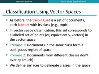
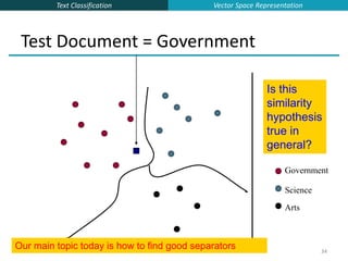
[log P(c j )  log P(xi |c j )
ipositions
 ]
Naïve Bayes

25. Text Classification
25
Two Naive Bayes Models
 Model 1: Multivariate Bernoulli
 One feature Xw for each word in dictionary
 Xw = true in document d if w appears in d
 Naive Bayes assumption:
 Given the document’s topic, appearance of one word in the
document tells us nothing about chances that another word
appears
 This is the model used in the binary independence
model in classic probabilistic relevance feedback on
hand-classified data (Maron in IR was a very early
user of NB)
Naïve Bayes

26. Text Classification
26
Two Models
 Model 2: Multinomial = Class conditional unigram
 One feature Xi for each word position in document
 feature’s values are all words in dictionary
 Value of Xi is the word in position i
 Naïve Bayes assumption:
 Given the document’s topic, word in one position in the document
tells us nothing about words in other positions
 Second assumption:
 Word appearance does not depend on position
 Just have one multinomial feature predicting all words
)
|
(
)
|
( c
w
X
P
c
w
X
P j
i 


for all positions i,j, word w, and class c
Naïve Bayes

27. Text Classification
27
 Multivariate Bernoulli model:
 Multinomial model:
 Can create a mega-document for topic j by concatenating all documents
in this topic
 Use frequency of w in mega-document
Parameter estimation
fraction of documents of topic cj
in which word w appears

 )
|
(
ˆ
j
w c
t
X
P
fraction of times in which
word w appears among all
words in documents of topic cj

 )
|
(
ˆ
j
i c
w
X
P
Naïve Bayes

28. Text Classification
28
Classification
 Multinomial vs Multivariate Bernoulli?
 Multinomial model is almost always more
effective in text applications!
 See results figures later
 See IIR sections 13.2 and 13.3 for worked
examples with each model
Naïve Bayes

29. Text Classification
29
29
The rest of text classification methods
 Vector space methods for Text Classification
 Vector space classification using centroids (Rocchio)
 K Nearest Neighbors
 Support Vector Machines

30. Text Classification
30
30
Recall: Vector Space Representation
 Each document is a vector, one component for each
term (= word).
 Normally normalize vectors to unit length.
 High-dimensional vector space:
 Terms are axes
 10,000+ dimensions, or even 100,000+
 Docs are vectors in this space
 How can we do classification in this space?
Vector Space Representation

31. Text Classification
31
31
Classification Using Vector Spaces
 As before, the training set is a set of documents,
each labeled with its class (e.g., topic)
 In vector space classification, this set corresponds to
a labeled set of points (or, equivalently, vectors) in
the vector space
 Premise 1: Documents in the same class form a
contiguous region of space
 Premise 2: Documents from different classes don’t
overlap (much)
 We define surfaces to delineate classes in the space
Vector Space Representation

32. Text Classification
32
32
Documents in a Vector Space
Government
Science
Arts
Vector Space Representation

33. Text Classification
33
33
Test Document of what class?
Government
Science
Arts
Vector Space Representation

34. Text Classification
34
34
Test Document = Government
Government
Science
Arts
Is this
similarity
hypothesis
true in
general?
Our main topic today is how to find good separators
Vector Space Representation

35. Text Classification
35
Rocchio Classification

36. Text Classification
36
Using Rocchio for text classification
 Relevance feedback methods can be adapted for
text categorization
 As noted before, relevance feedback can be viewed as 2-
class classification
 Relevant vs. nonrelevant documents
 Use standard tf-idf weighted vectors to represent
text documents
 For training documents in each category, compute a
prototype vector by summing the vectors of the
training documents in the category.
 Prototype = centroid of members of class
 Assign test documents to the category with the
closest prototype vector based on cosine similarity.
36
Rocchio Classification

37. Text Classification
37
Illustration of Rocchio Text Categorization
37
Rocchio Classification

38. Text Classification
38
Definition of centroid
 Where Dc is the set of all documents that belong to
class c and v(d) is the vector space representation of
d.
 Note that centroid will in general not be a unit vector
even when the inputs are unit vectors.
38

(c) 
1
| Dc |
v(d)
d Dc

Rocchio Classification

39. Text Classification
39
39
Rocchio Properties
 Forms a simple generalization of the examples in
each class (a prototype).
 Prototype vector does not need to be averaged or
otherwise normalized for length since cosine
similarity is insensitive to vector length.
 Classification is based on similarity to class
prototypes.
 Does not guarantee classifications are consistent
with the given training data.
Why not?
Rocchio Classification

40. Text Classification
40
40
Rocchio Anomaly
 Prototype models have problems with polymorphic
(disjunctive) categories.
Rocchio Classification

41. Text Classification
41
Rocchio classification
 Rocchio forms a simple representation for each class:
the centroid/prototype
 Classification is based on similarity to / distance from
the prototype/centroid
 It does not guarantee that classifications are
consistent with the given training data
 It is little used outside text classification
 It has been used quite effectively for text classification
 But in general worse than Naïve Bayes
 Again, cheap to train and test documents
41
Rocchio Classification

42. Text Classification
42
kNN Classification

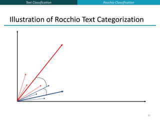
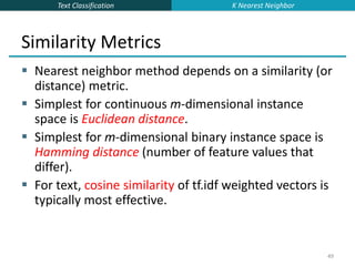
43. Text Classification
43
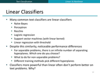
43
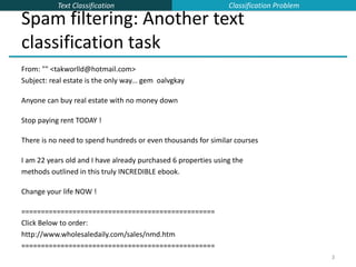
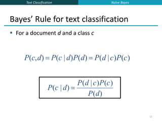
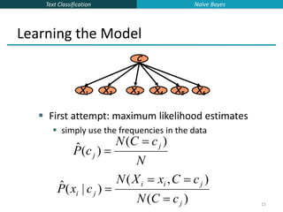
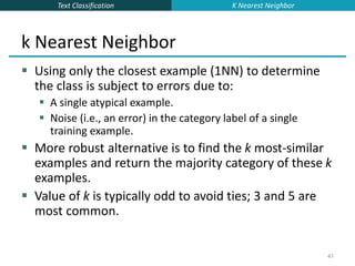
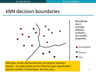
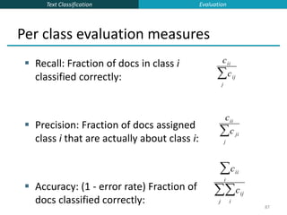
k Nearest Neighbor Classification
 kNN = k Nearest Neighbor
 To classify a document d into class c:
 Define k-neighborhood N as k nearest neighbors of d
 Count number of documents ic in N that belong to c
 Estimate P(c|d) as ic/k
 Choose as class argmaxc P(c|d) [ = majority class]
K Nearest Neighbor

44. Text Classification
44
44
Example: k=6 (6NN)
Government
Science
Arts
P(science| )?
K Nearest Neighbor

45. Text Classification
45
45
Nearest-Neighbor Learning Algorithm
 Learning is just storing the representations of the training examples
in D.
 Testing instance x (under 1NN):
 Compute similarity between x and all examples in D.
 Assign x the category of the most similar example in D.
 Does not explicitly compute a generalization or category prototypes.
 Also called:
 Case-based learning
 Memory-based learning
 Lazy learning
 Rationale of kNN: contiguity hypothesis
K Nearest Neighbor

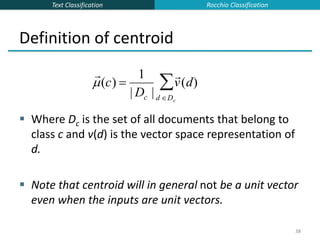
46. Text Classification
46
46
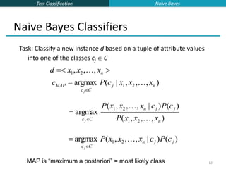
kNN Is Close to Optimal
 Cover and Hart (1967)
 Asymptotically, the error rate of 1-nearest-neighbor
classification is less than twice the Bayes rate [error rate of
classifier knowing model that generated data]
 In particular, asymptotic error rate is 0 if Bayes rate is
0.
 Assume: query point coincides with a training point.
 Both query point and training point contribute error
→ 2 times Bayes rate
K Nearest Neighbor

47. Text Classification
47
47
k Nearest Neighbor
 Using only the closest example (1NN) to determine
the class is subject to errors due to:
 A single atypical example.
 Noise (i.e., an error) in the category label of a single
training example.
 More robust alternative is to find the k most-similar
examples and return the majority category of these k
examples.
 Value of k is typically odd to avoid ties; 3 and 5 are
most common.
K Nearest Neighbor

48. Text Classification
48
48
kNN decision boundaries
Government
Science
Arts
Boundaries
are in
principle
arbitrary
surfaces –
but usually
polyhedra
kNN gives locally defined decision boundaries between
classes – far away points do not influence each classification
decision (unlike in Naïve Bayes, Rocchio, etc.)
K Nearest Neighbor

49. Text Classification
49
49
Similarity Metrics
 Nearest neighbor method depends on a similarity (or
distance) metric.
 Simplest for continuous m-dimensional instance
space is Euclidean distance.
 Simplest for m-dimensional binary instance space is
Hamming distance (number of feature values that
differ).
 For text, cosine similarity of tf.idf weighted vectors is
typically most effective.
K Nearest Neighbor

50. Text Classification
50
50
Illustration of 3 Nearest Neighbor for Text
Vector Space
K Nearest Neighbor

51. Text Classification
51
51
3 Nearest Neighbor vs. Rocchio
 Nearest Neighbor tends to handle polymorphic
categories better than Rocchio/NB.
K Nearest Neighbor

52. Text Classification
52
52
Nearest Neighbor with Inverted Index
 Naively finding nearest neighbors requires a linear
search through |D| documents in collection
 But determining k nearest neighbors is the same as
determining the k best retrievals using the test
document as a query to a database of training
documents.
 Use standard vector space inverted index methods to
find the k nearest neighbors.
 Testing Time: O(B|Vt|) where B is the average
number of training documents in which a test-document word
appears.
 Typically B << |D|
K Nearest Neighbor

53. Text Classification
53
53
kNN: Discussion
 Scales well with large number of classes
 Don’t need to train n classifiers for n classes
 Classes can influence each other
 Small changes to one class can have ripple effect
 Scores can be hard to convert to probabilities
 No training necessary
 Actually: perhaps not true. (Data editing, etc.)
 May be expensive at test time
 In most cases it’s more accurate than NB or Rocchio
K Nearest Neighbor

54. Text Classification
54
Support Vector Machine

55. Text Classification
55
55
Linear classifiers and binary and multiclass
classification
 Consider 2 class problems
 Deciding between two classes, perhaps, government and
non-government
 One-versus-rest classification
 How do we define (and find) the separating surface?
 How do we decide which region a test doc is in?

56. Text Classification
56
56
Linear classifier: Example
 Class: “interest” (as in interest rate)
 Example features of a linear classifier
 wi ti wi ti
 To classify, find dot product of feature vector and weights
• 0.70 prime
• 0.67 rate
• 0.63 interest
• 0.60 rates
• 0.46 discount
• 0.43 bundesbank
• −0.71 dlrs
• −0.35 world
• −0.33 sees
• −0.25 year
• −0.24 group
• −0.24 dlr
Linear Vs Nonlinear

57. Text Classification
57
57
Linear Classifiers
 Many common text classifiers are linear classifiers
 Naïve Bayes
 Perceptron
 Rocchio
 Logistic regression
 Support vector machines (with linear kernel)
 Linear regression with threshold
 Despite this similarity, noticeable performance differences
 For separable problems, there is an infinite number of separating
hyperplanes. Which one do you choose?
 What to do for non-separable problems?
 Different training methods pick different hyperplanes
 Classifiers more powerful than linear often don’t perform better on
text problems. Why?
Linear Vs Nonlinear

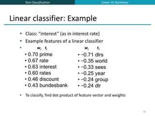
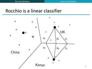
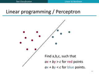
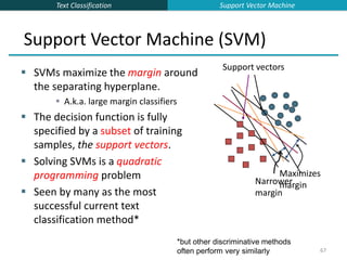
58. Text Classification
58
Two-class Rocchio as a linear classifier
 Line or hyperplane defined by:
 For Rocchio, set:
[Aside for ML/stats people: Rocchio classification is a simplification of the classic Fisher
Linear Discriminant where you don’t model the variance (or assume it is spherical).]
58

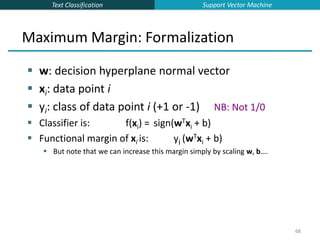
widi  
i1
M


w  (c1)  (c2)
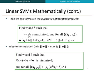
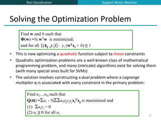
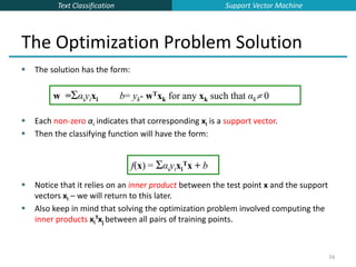
  0.5  (| (c1) |2
 | (c2) |2
)
Linear Vs Nonlinear

59. Text Classification
59
Rocchio is a linear classifier
59
Linear Vs Nonlinear

60. Text Classification
60
60
Naive Bayes is a linear classifier
 Two-class Naive Bayes. We compute:
 Decide class C if the odds is greater than 1, i.e., if the
log odds is greater than 0.
 So decision boundary is hyperplane:
d
w
#
n
C
w
P
C
w
P
C
P
C
P
n
w
w
w
V
w w
in
of
s
occurrence
of
;
)
|
(
)
|
(
log
;
)
(
)
(
log
where
0





  




( | ) ( ) ( | )
log log log
( | ) ( ) ( | )
w d
P C d P C P w C
P C d P C P w C

  
Linear Vs Nonlinear

61. Text Classification
61
A nonlinear problem
 A linear classifier
like Naïve Bayes
does badly on
this task
 kNN will do very
well (assuming
enough training
data)
61
Linear Vs Nonlinear

62. Text Classification
62
62
Separation by Hyperplanes
 A strong high-bias assumption is linear separability:
 in 2 dimensions, can separate classes by a line
 in higher dimensions, need hyperplanes
 Can find separating hyperplane by linear programming
(or can iteratively fit solution via perceptron):
 separator can be expressed as ax + by = c
Linear Vs Nonlinear

63. Text Classification
63
63
Linear programming / Perceptron
Find a,b,c, such that
ax + by > c for red points
ax + by < c for blue points.
Linear Vs Nonlinear

64. Text Classification
64
64
Which Hyperplane?
In general, lots of possible
solutions for a,b,c.
Linear Vs Nonlinear

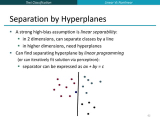
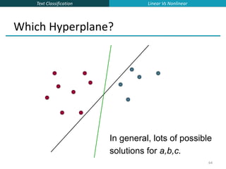
65. Text Classification
65
65
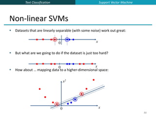
Which Hyperplane?
 Lots of possible solutions for a,b,c.
 Some methods find a separating hyperplane,
but not the optimal one [according to some
criterion of expected goodness]
 E.g., perceptron
 Most methods find an optimal separating
hyperplane
 Which points should influence optimality?
 All points
 Linear/logistic regression
 Naïve Bayes
 Only “difficult points” close to decision
boundary
 Support vector machines
Linear Vs Nonlinear

66. Text Classification
66
66
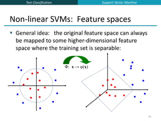
Linear classifiers: Which Hyperplane?
 Lots of possible solutions for a, b, c.
 Some methods find a separating hyperplane,
but not the optimal one [according to some
criterion of expected goodness]
 E.g., perceptron
 Support Vector Machine (SVM) finds an
optimal solution.
 Maximizes the distance between the
hyperplane and the “difficult points” close to
decision boundary
 One intuition: if there are no points near the
decision surface, then there are no very
uncertain classification decisions
This line represents
the decision
boundary:
ax + by − c = 0
Support Vector Machine

67. Text Classification
67
67
Support Vector Machine (SVM)
Support vectors
Maximizes
margin
 SVMs maximize the margin around
the separating hyperplane.
 A.k.a. large margin classifiers
 The decision function is fully
specified by a subset of training
samples, the support vectors.
 Solving SVMs is a quadratic
programming problem
 Seen by many as the most
successful current text
classification method*
*but other discriminative methods
often perform very similarly
Narrower
margin
Support Vector Machine

68. Text Classification
68
68
 w: decision hyperplane normal vector
 xi: data point i
 yi: class of data point i (+1 or -1) NB: Not 1/0
 Classifier is: f(xi) = sign(wTxi + b)
 Functional margin of xi is: yi (wTxi + b)
 But note that we can increase this margin simply by scaling w, b….
Maximum Margin: Formalization
Support Vector Machine

69. Text Classification
69
69
Geometric Margin
 Distance from example to the separator is
 Examples closest to the hyperplane are support vectors.
 Margin ρ of the separator is the width of separation between support vectors
of classes.
w
x
w b
y
r
T


r
ρ
x
x’
w
Derivation of finding r:
Dotted line x’−x is perpendicular to
decision boundary so parallel to w.
Unit vector is w/||w||, so line is rw/||w||.
x’ = x – yrw/||w||.
x’ satisfies wTx’+b = 0.
So wT(x –yrw/||w||) + b = 0
Recall that ||w|| = sqrt(wTw).
So, solving for r gives:
r = y(wTx + b)/||w||
Support Vector Machine

70. Text Classification
70
70
Linear SVM Mathematically
The linearly separable case
 Assume that all data is at least distance 1 from the hyperplane, then the
following two constraints follow for a training set {(xi ,yi)}
 For support vectors, the inequality becomes an equality
 Then, since each example’s distance from the hyperplane is
 The margin is:
wTxi + b ≥ 1 if yi = 1
wTxi + b ≤ -1 if yi = -1
w
2


w
x
w b
y
r
T


Support Vector Machine

71. Text Classification
71
71
Linear Support Vector Machine (SVM)
 Hyperplane
wT x + b = 0
 Extra scale constraint:
mini=1,…,n |wTxi + b| = 1
 This implies:
wT(xa–xb) = 2
ρ = ||xa–xb||2 = 2/||w||2
wT x + b = 0
wTxa + b = 1
wTxb + b = -1
ρ
Support Vector Machine

72. Text Classification
72
72
Linear SVMs Mathematically (cont.)
 Then we can formulate the quadratic optimization problem:
 A better formulation (min ||w|| = max 1/ ||w|| ):
Find w and b such that
is maximized; and for all {(xi , yi)}
wTxi + b ≥ 1 if yi=1; wTxi + b ≤ -1 if yi = -1
w
2


Find w and b such that
Φ(w) =½ wTw is minimized;
and for all {(xi ,yi)}: yi (wTxi + b) ≥ 1
Support Vector Machine

73. Text Classification
73
73
Solving the Optimization Problem
 This is now optimizing a quadratic function subject to linear constraints
 Quadratic optimization problems are a well-known class of mathematical
programming problem, and many (intricate) algorithms exist for solving them
(with many special ones built for SVMs)
 The solution involves constructing a dual problem where a Lagrange
multiplier αi is associated with every constraint in the primary problem:
Find w and b such that
Φ(w) =½ wTw is minimized;
and for all {(xi ,yi)}: yi (wTxi + b) ≥ 1
Find α1…αN such that
Q(α) =Σαi - ½ΣΣαiαjyiyjxi
Txj is maximized and
(1) Σαiyi = 0
(2) αi ≥ 0 for all αi
Support Vector Machine

74. Text Classification
74
74
The Optimization Problem Solution
 The solution has the form:
 Each non-zero αi indicates that corresponding xi is a support vector.
 Then the classifying function will have the form:
 Notice that it relies on an inner product between the test point x and the support
vectors xi – we will return to this later.
 Also keep in mind that solving the optimization problem involved computing the
inner products xi
Txj between all pairs of training points.
w =Σαiyixi b= yk- wTxk for any xk such that αk 0
f(x) = Σαiyixi
Tx + b
Support Vector Machine

75. Text Classification
75
75
Soft Margin Classification
 If the training data is not
linearly separable, slack
variables ξi can be added to
allow misclassification of
difficult or noisy examples.
 Allow some errors
 Let some points be moved
to where they belong, at a
cost
 Still, try to minimize training
set errors, and to place
hyperplane “far” from each
class (large margin)
ξj
ξi
Support Vector Machine

76. Text Classification
76
76
Soft Margin Classification
Mathematically
 The old formulation:
 The new formulation incorporating slack variables:
 Parameter C can be viewed as a way to control overfitting – a
regularization term
Find w and b such that
Φ(w) =½ wTw is minimized and for all {(xi ,yi)}
yi (wTxi + b) ≥ 1
Find w and b such that
Φ(w) =½ wTw + CΣξi is minimized and for all {(xi ,yi)}
yi (wTxi + b) ≥ 1- ξi and ξi ≥ 0 for all i
Support Vector Machine

77. Text Classification
77
77
Soft Margin Classification – Solution
 The dual problem for soft margin classification:
 Neither slack variables ξi nor their Lagrange multipliers appear in the dual problem!
 Again, xi with non-zero αi will be support vectors.
 Solution to the dual problem is:
Find α1…αN such that
Q(α) =Σαi - ½ΣΣαiαjyiyjxi
Txj is maximized and
(1) Σαiyi = 0
(2) 0 ≤ αi ≤ C for all αi
w = Σαiyixi
b = yk(1- ξk) - wTxk where k = argmax αk’
k’ f(x) = Σαiyixi
Tx + b
w is not needed explicitly for
classification!
Support Vector Machine

78. Text Classification
78
78
Classification with SVMs
 Given a new point x, we can score its projection
onto the hyperplane normal:
 I.e., compute score: wTx + b = Σαiyixi
Tx + b
 Can set confidence threshold t.
-1
0
1
Score > t: yes
Score < -t: no
Else: don’t know
Support Vector Machine

79. Text Classification
79
79
Linear SVMs: Summary
 The classifier is a separating hyperplane.
 The most “important” training points are the support vectors; they define
the hyperplane.
 Quadratic optimization algorithms can identify which training points xi are
support vectors with non-zero Lagrangian multipliers αi.
 Both in the dual formulation of the problem and in the solution, training
points appear only inside inner products:
Find α1…αN such that
Q(α) =Σαi - ½ΣΣαiαjyiyjxi
Txj is maximized and
(1) Σαiyi = 0
(2) 0 ≤ αi ≤ C for all αi
f(x) = Σαiyixi
Tx + b
Support Vector Machine

80. Text Classification
80
80
Non-linear SVMs
 Datasets that are linearly separable (with some noise) work out great:
 But what are we going to do if the dataset is just too hard?
 How about … mapping data to a higher-dimensional space:
0
x2
x
0 x
0 x
Support Vector Machine

81. Text Classification
81
81
Non-linear SVMs: Feature spaces
 General idea: the original feature space can always
be mapped to some higher-dimensional feature
space where the training set is separable:
Φ: x → φ(x)
Support Vector Machine

82. Text Classification
82
82
The “Kernel Trick”
 The linear classifier relies on an inner product between vectors K(xi,xj)=xi
Txj
 If every data point is mapped into high-dimensional space via some
transformation Φ: x → φ(x), the inner product becomes:
K(xi,xj)= φ(xi) Tφ(xj)
 A kernel function is some function that corresponds to an inner product in
some expanded feature space.
 Example:
2-dimensional vectors x=[x1 x2]; let K(xi,xj)=(1 + xi
Txj)2
,
Need to show that K(xi,xj)= φ(xi) Tφ(xj):
K(xi,xj)=(1 + xi
Txj)2
,= 1+ xi1
2xj1
2 + 2 xi1xj1 xi2xj2+ xi2
2xj2
2 + 2xi1xj1 + 2xi2xj2=
= [1 xi1
2 √2 xi1xi2 xi2
2 √2xi1 √2xi2]T [1 xj1
2 √2 xj1xj2 xj2
2 √2xj1 √2xj2]
= φ(xi)Tφ(xj) where φ(x) = [1 x1
2 √2 x1x2 x2
2 √2x1 √2x2]
Support Vector Machine

83. Text Classification
83
83
Kernels
 Why use kernels?
 Make non-separable problem separable.
 Map data into better representational space
 Common kernels
 Linear
 Polynomial K(x,z) = (1+xTz)d
 Gives feature conjunctions
 Radial basis function (infinite dimensional space)
 Haven’t been very useful in text classification
Support Vector Machine

84. Text Classification
84
84
 Most (over)used data set
 21578 documents
 9603 training, 3299 test articles (ModApte/Lewis split)
 118 categories
 An article can be in more than one category
 Learn 118 binary category distinctions
 Average document: about 90 types, 200 tokens
 Average number of classes assigned
 1.24 for docs with at least one category
 Only about 10 out of 118 categories are large
Common categories
(#train, #test)
Evaluation: Classic Reuters-21578 Data Set
• Earn (2877, 1087)
• Acquisitions (1650, 179)
• Money-fx (538, 179)
• Grain (433, 149)
• Crude (389, 189)
• Trade (369,119)
• Interest (347, 131)
• Ship (197, 89)
• Wheat (212, 71)
• Corn (182, 56)
Evaluation

85. Text Classification
85
85
Reuters Text Categorization data set
(Reuters-21578) document
<REUTERS TOPICS="YES" LEWISSPLIT="TRAIN" CGISPLIT="TRAINING-SET"
OLDID="12981" NEWID="798">
<DATE> 2-MAR-1987 16:51:43.42</DATE>
<TOPICS><D>livestock</D><D>hog</D></TOPICS>
<TITLE>AMERICAN PORK CONGRESS KICKS OFF TOMORROW</TITLE>
<DATELINE> CHICAGO, March 2 - </DATELINE><BODY>The American Pork Congress
kicks off tomorrow, March 3, in Indianapolis with 160 of the nations pork producers from 44
member states determining industry positions on a number of issues, according to the National Pork
Producers Council, NPPC.
Delegates to the three day Congress will be considering 26 resolutions concerning various issues,
including the future direction of farm policy and the tax law as it applies to the agriculture sector.
The delegates will also debate whether to endorse concepts of a national PRV (pseudorabies virus)
control and eradication program, the NPPC said.
A large trade show, in conjunction with the congress, will feature the latest in technology in all
areas of the industry, the NPPC added. Reuter
&#3;</BODY></TEXT></REUTERS>
Evaluation

86. Text Classification
86
86
Good practice department:
Confusion matrix
 In a perfect classification, only the diagonal has non-zero
entries
53
Class assigned by classifier
Actual
Class
This (i, j) entry of the confusion matrix means of the
points actually in class i were put in class j by the
classifier.
Evaluation
ij
c
c

87. Text Classification
87
87
Per class evaluation measures
 Recall: Fraction of docs in class i
classified correctly:
 Precision: Fraction of docs assigned
class i that are actually about class i:
 Accuracy: (1 - error rate) Fraction of
docs classified correctly:
cii
i

cij
i

j


cii
c ji
j


cii
cij
j

Evaluation

88. Text Classification
88
88
Micro- vs. Macro-Averaging
 If we have more than one class, how do we combine
multiple performance measures into one quantity?
 Macroaveraging: Compute performance for each
class, then average.
 Microaveraging: Collect decisions for all classes,
compute contingency table, evaluate.
Evaluation

89. Text Classification
89
89
Micro- vs. Macro-Averaging: Example
Classifi
er: yes
Classifi
er: no
Truth:
yes
10 10
Truth:
no
30 970
Classifi
er: yes
Classifi
er: no
Truth:
yes
90 10
Truth:
no
10 890
Classifi
er: yes
Classifi
er: no
Truth: yes 100 20
Truth: no 40 1860
Class 1 Class 2 Micro Ave. Table
 Macroaveraged precision: (0.25 + 0.9)/2
 Microaveraged precision: 100/140
 Microaveraged score is dominated by score on
common classes
Evaluation
Confusion matrices:

90. Text Classification
90
90
Evaluation

91. Text Classification
91
Precision-recall for category: Crude
0
0.1
0.2
0.3
0.4
0.5
0.6
0.7
0.8
0.9
1
0 0.2 0.4 0.6 0.8 1
LSVM
Decision Tree
Naïve Bayes
Rocchio
Precision
Recall
Dumais
(1998)
Evaluation

92. Text Classification
92
92
Precision-recall for category: Ship
Precision
Recall
0
0.1
0.2
0.3
0.4
0.5
0.6
0.7
0.8
0.9
1
0 0.2 0.4 0.6 0.8 1
LSVM
Decision Tree
Naïve Bayes
Rocchio
Dumais
(1998)
Evaluation

93. Text Classification
93
93
Yang&Liu: SVM vs. Other Methods
Evaluation

94. Text Classification
94
94
Resources
 IIR 13-15
 Fabrizio Sebastiani. Machine Learning in Automated Text
Categorization. ACM Computing Surveys, 34(1):1-47, 2002.
 Yiming Yang & Xin Liu, A re-examination of text categorization
methods. Proceedings of SIGIR, 1999.
 Trevor Hastie, Robert Tibshirani and Jerome Friedman,
Elements of Statistical Learning: Data Mining, Inference and
Prediction. Springer-Verlag, New York.
 Open Calais: Automatic Semantic Tagging
 Free (but they can keep your data), provided by Thompson/Reuters
 Weka: A data mining software package that includes an
implementation of many ML algorithms