This document serves as an introduction to information retrieval principles, focusing on scoring, term weighting, and the vector space model. It discusses the shortcomings of boolean search methods and presents ranked retrieval as a more effective approach to handling user queries, highlighting various scoring methods like the Jaccard coefficient, term frequency, and TF-IDF weighting. Additionally, it covers concepts such as document vectors in high-dimensional space and cosine similarity for ranking relevant documents.

1. Introduction to Information Retrieval
Introduction to
Information Retrieval
CS276: Information Retrieval and Web Search
Pandu Nayak and Prabhakar Raghavan
Lecture 6: Scoring, Term Weighting and the
Vector Space Model

2. Introduction to Information Retrieval
Recap of lecture 5
 Collection and vocabulary statistics: Heaps’ and Zipf’s laws
 Dictionary compression for Boolean indexes
 Dictionary string, blocks, front coding
 Postings compression: Gap encoding, prefix-unique codes
 Variable-Byte and Gamma codes
collection (text, xml markup etc) 3,600.0
collection (text) 960.0
Term-doc incidence matrix 40,000.0
postings, uncompressed (32-bit words) 400.0
postings, uncompressed (20 bits) 250.0
postings, variable byte encoded 116.0
postings, encoded 101.0
MB

3. Introduction to Information Retrieval
This lecture; IIR Sections 6.2-6.4.3
 Ranked retrieval
 Scoring documents
 Term frequency
 Collection statistics
 Weighting schemes
 Vector space scoring

4. Introduction to Information Retrieval
Ranked retrieval
 Thus far, our queries have all been Boolean.
 Documents either match or don’t.
 Good for expert users with precise understanding of
their needs and the collection.
 Also good for applications: Applications can easily
consume 1000s of results.
 Not good for the majority of users.
 Most users incapable of writing Boolean queries (or they
are, but they think it’s too much work).
 Most users don’t want to wade through 1000s of results.
 This is particularly true of web search.
Ch. 6

5. Introduction to Information Retrieval
Problem with Boolean search:
feast or famine
 Boolean queries often result in either too few (=0) or
too many (1000s) results.
 Query 1: “standard user dlink 650” → 200,000 hits
 Query 2: “standard user dlink 650 no card found”: 0
hits
 It takes a lot of skill to come up with a query that
produces a manageable number of hits.
 AND gives too few; OR gives too many
Ch. 6

6. Introduction to Information Retrieval
Ranked retrieval models
 Rather than a set of documents satisfying a query
expression, in ranked retrieval, the system returns an
ordering over the (top) documents in the collection
for a query
 Free text queries: Rather than a query language of
operators and expressions, the user’s query is just
one or more words in a human language
 In principle, there are two separate choices here, but
in practice, ranked retrieval has normally been
associated with free text queries and vice versa
6

7. Introduction to Information Retrieval
Feast or famine: not a problem in
ranked retrieval
 When a system produces a ranked result set, large
result sets are not an issue
 Indeed, the size of the result set is not an issue
 We just show the top k ( ≈ 10) results
 We don’t overwhelm the user
 Premise: the ranking algorithm works
Ch. 6

8. Introduction to Information Retrieval
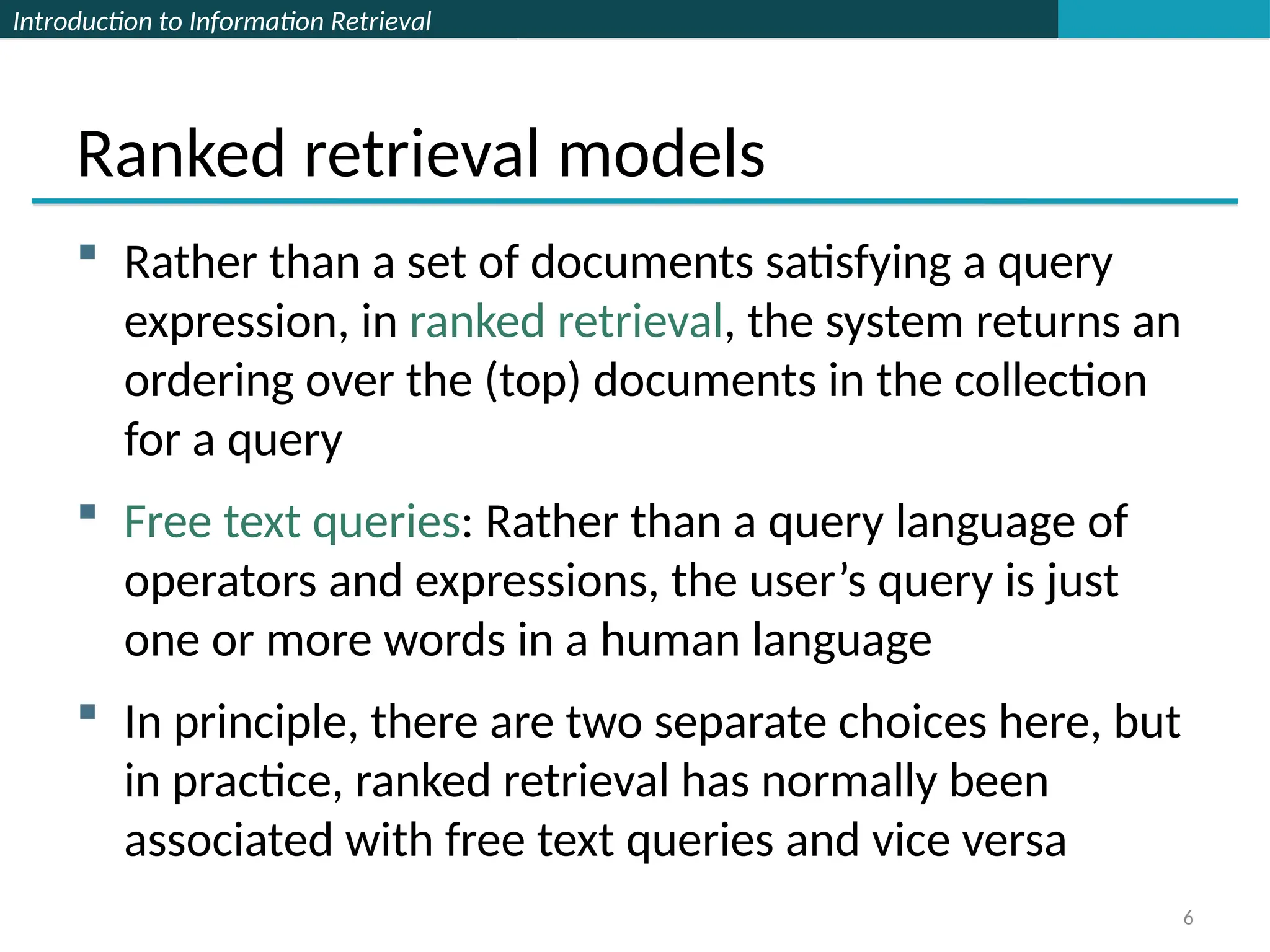
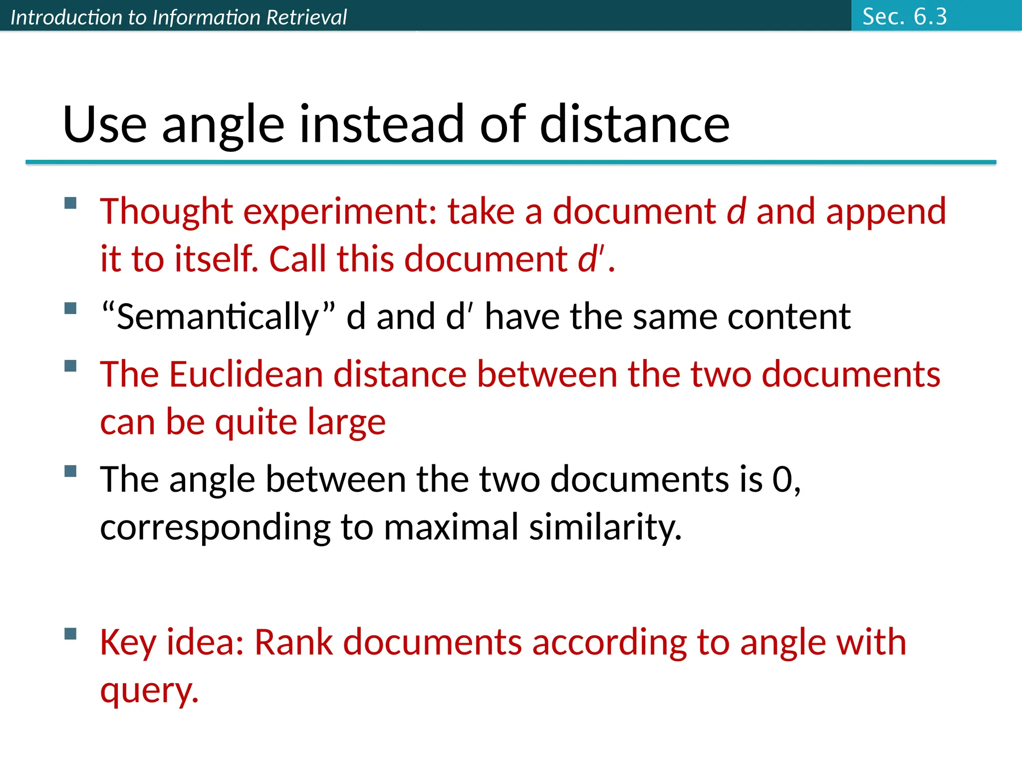
Scoring as the basis of ranked retrieval
 We wish to return in order the documents most likely
to be useful to the searcher
 How can we rank-order the documents in the
collection with respect to a query?
 Assign a score – say in [0, 1] – to each document
 This score measures how well document and query
“match”.
Ch. 6

9. Introduction to Information Retrieval
Query-document matching scores
 We need a way of assigning a score to a
query/document pair
 Let’s start with a one-term query
 If the query term does not occur in the document:
score should be 0
 The more frequent the query term in the document,
the higher the score (should be)
 We will look at a number of alternatives for this.
Ch. 6

10. Introduction to Information Retrieval
Take 1: Jaccard coefficient
 Recall from Lecture 3: A commonly used measure of
overlap of two sets A and B
 jaccard(A,B) = |A ∩ B| / |A ∪ B|
 jaccard(A,A) = 1
 jaccard(A,B) = 0 if A ∩ B = 0
 A and B don’t have to be the same size.
 Always assigns a number between 0 and 1.
Ch. 6

11. Introduction to Information Retrieval
Jaccard coefficient: Scoring example
 What is the query-document match score that the
Jaccard coefficient computes for each of the two
documents below?
 Query: ides of march
 Document 1: caesar died in march
 Document 2: the long march
Ch. 6

12. Introduction to Information Retrieval
Issues with Jaccard for scoring
 It doesn’t consider term frequency (how many times
a term occurs in a document)
 Rare terms in a collection are more informative than
frequent terms. Jaccard doesn’t consider this
information
 We need a more sophisticated way of normalizing for
length
 Later in this lecture, we’ll use
 . . . instead of |A ∩ B|/|A B| (Jaccard) for length
∪
normalization.
|
B
A
|
/
|
B
A
| 

Ch. 6

13. Introduction to Information Retrieval
Recall (Lecture 1): Binary term-
document incidence matrix
Antony and Cleopatra Julius Caesar The Tempest Hamlet Othello Macbeth
Antony 1 1 0 0 0 1
Brutus 1 1 0 1 0 0
Caesar 1 1 0 1 1 1
Calpurnia 0 1 0 0 0 0
Cleopatra 1 0 0 0 0 0
mercy 1 0 1 1 1 1
worser 1 0 1 1 1 0
Each document is represented by a binary vector {0,1}
∈ |V|
Sec. 6.2

14. Introduction to Information Retrieval
Term-document count matrices
 Consider the number of occurrences of a term in a
document:
 Each document is a count vector in ℕv
: a column below
Antony and Cleopatra Julius Caesar The Tempest Hamlet Othello Macbeth
Antony 157 73 0 0 0 0
Brutus 4 157 0 1 0 0
Caesar 232 227 0 2 1 1
Calpurnia 0 10 0 0 0 0
Cleopatra 57 0 0 0 0 0
mercy 2 0 3 5 5 1
worser 2 0 1 1 1 0
Sec. 6.2

15. Introduction to Information Retrieval
Bag of words model
 Vector representation doesn’t consider the ordering
of words in a document
 John is quicker than Mary and Mary is quicker than
John have the same vectors
 This is called the bag of words model.
 In a sense, this is a step back: The positional index
was able to distinguish these two documents.
 We will look at “recovering” positional information
later in this course.
 For now: bag of words model

16. Introduction to Information Retrieval
Term frequency tf
 The term frequency tft,d of term t in document d is
defined as the number of times that t occurs in d.
 We want to use tf when computing query-document
match scores. But how?
 Raw term frequency is not what we want:
 A document with 10 occurrences of the term is more
relevant than a document with 1 occurrence of the term.
 But not 10 times more relevant.
 Relevance does not increase proportionally with
term frequency.
NB: frequency = count in IR

17. Introduction to Information Retrieval
Log-frequency weighting
 The log frequency weight of term t in d is
 0 → 0, 1 → 1, 2 → 1.3, 10 → 2, 1000 → 4, etc.
 Score for a document-query pair: sum over terms t in
both q and d:
 score
 The score is 0 if none of the query terms is present in
the document.


 


otherwise
0,
0
tf
if
,
tf
log
1 10 t,d
t,d
t,d
w
 


 d
q
t d
t )
tf
log
(1 ,
Sec. 6.2

18. Introduction to Information Retrieval
Document frequency
 Rare terms are more informative than frequent terms
 Recall stop words
 Consider a term in the query that is rare in the
collection (e.g., arachnocentric)
 A document containing this term is very likely to be
relevant to the query arachnocentric
 → We want a high weight for rare terms like
arachnocentric.
Sec. 6.2.1

19. Introduction to Information Retrieval
Document frequency, continued
 Frequent terms are less informative than rare terms
 Consider a query term that is frequent in the
collection (e.g., high, increase, line)
 A document containing such a term is more likely to
be relevant than a document that doesn’t
 But it’s not a sure indicator of relevance.
 → For frequent terms, we want high positive weights
for words like high, increase, and line
 But lower weights than for rare terms.
 We will use document frequency (df) to capture this.
Sec. 6.2.1

20. Introduction to Information Retrieval
idf weight
 dft is the document frequency of t: the number of
documents that contain t
 dft is an inverse measure of the informativeness of t
 dft  N
 We define the idf (inverse document frequency) of t
by
 We use log (N/dft) instead of N/dft to “dampen” the effect
of idf.
)
/df
(
log
idf 10 t
t N

Will turn out the base of the log is immaterial.
Sec. 6.2.1

21. Introduction to Information Retrieval
idf example, suppose N = 1 million
term dft idft
calpurnia 1
animal 100
sunday 1,000
fly 10,000
under 100,000
the 1,000,000
There is one idf value for each term t in a collection.
Sec. 6.2.1
)
/df
(
log
idf 10 t
t N


22. Introduction to Information Retrieval
Effect of idf on ranking
 Does idf have an effect on ranking for one-term
queries, like
 iPhone
 idf has no effect on ranking one term queries
 idf affects the ranking of documents for queries with at
least two terms
 For the query capricious person, idf weighting makes
occurrences of capricious count for much more in the final
document ranking than occurrences of person.
22

23. Introduction to Information Retrieval
Collection vs. Document frequency
 The collection frequency of t is the number of
occurrences of t in the collection, counting
multiple occurrences.
 Example:
 Which word is a better search term (and should
get a higher weight)?
Word Collection frequency Document frequency
insurance 10440 3997
try 10422 8760
Sec. 6.2.1

24. Introduction to Information Retrieval
tf-idf weighting
 The tf-idf weight of a term is the product of its tf
weight and its idf weight.
 Best known weighting scheme in information retrieval
 Note: the “-” in tf-idf is a hyphen, not a minus sign!
 Alternative names: tf.idf, tf x idf
 Increases with the number of occurrences within a
document
 Increases with the rarity of the term in the collection
)
df
/
(
log
)
tf
1
log(
w 10
,
, t
d
t N
d
t



Sec. 6.2.2

25. Introduction to Information Retrieval
Score for a document given a query
 There are many variants
 How “tf” is computed (with/without logs)
 Whether the terms in the query are also weighted
 …
25
Score(q,d)  tf.idft,d
tqd

Sec. 6.2.2

26. Introduction to Information Retrieval
Binary → count → weight matrix
Antony and Cleopatra Julius Caesar The Tempest Hamlet Othello Macbeth
Antony 5.25 3.18 0 0 0 0.35
Brutus 1.21 6.1 0 1 0 0
Caesar 8.59 2.54 0 1.51 0.25 0
Calpurnia 0 1.54 0 0 0 0
Cleopatra 2.85 0 0 0 0 0
mercy 1.51 0 1.9 0.12 5.25 0.88
worser 1.37 0 0.11 4.15 0.25 1.95
Each document is now represented by a real-valued
vector of tf-idf weights ∈ R|V|
Sec. 6.3

27. Introduction to Information Retrieval
Documents as vectors
 So we have a |V|-dimensional vector space
 Terms are axes of the space
 Documents are points or vectors in this space
 Very high-dimensional: tens of millions of dimensions
when you apply this to a web search engine
 These are very sparse vectors - most entries are zero.
Sec. 6.3

28. Introduction to Information Retrieval
Queries as vectors
 Key idea 1: Do the same for queries: represent them
as vectors in the space
 Key idea 2: Rank documents according to their
proximity to the query in this space
 proximity = similarity of vectors
 proximity ≈ inverse of distance
 Recall: We do this because we want to get away from
the you’re-either-in-or-out Boolean model.
 Instead: rank more relevant documents higher than
less relevant documents
Sec. 6.3

29. Introduction to Information Retrieval
Formalizing vector space proximity
 First cut: distance between two points
 ( = distance between the end points of the two vectors)
 Euclidean distance?
 Euclidean distance is a bad idea . . .
 . . . because Euclidean distance is large for vectors of
different lengths.
Sec. 6.3

30. Introduction to Information Retrieval
Why distance is a bad idea
The Euclidean
distance between q
and d2 is large even
though the
distribution of terms
in the query q and the
distribution of
terms in the
document d2 are
very similar.
Sec. 6.3

31. Introduction to Information Retrieval
Use angle instead of distance
 Thought experiment: take a document d and append
it to itself. Call this document d .
′
 “Semantically” d and d have the same content
′
 The Euclidean distance between the two documents
can be quite large
 The angle between the two documents is 0,
corresponding to maximal similarity.
 Key idea: Rank documents according to angle with
query.
Sec. 6.3

32. Introduction to Information Retrieval
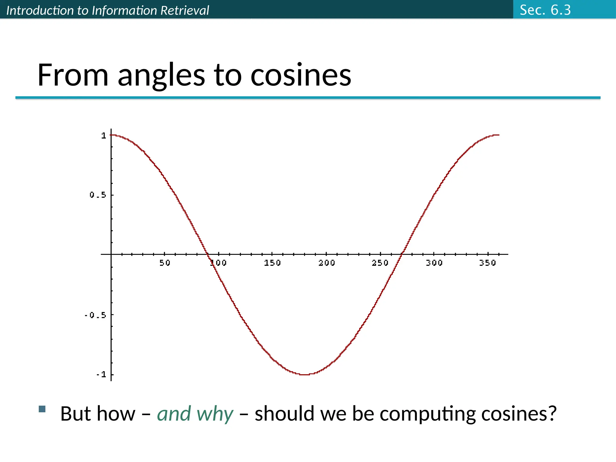
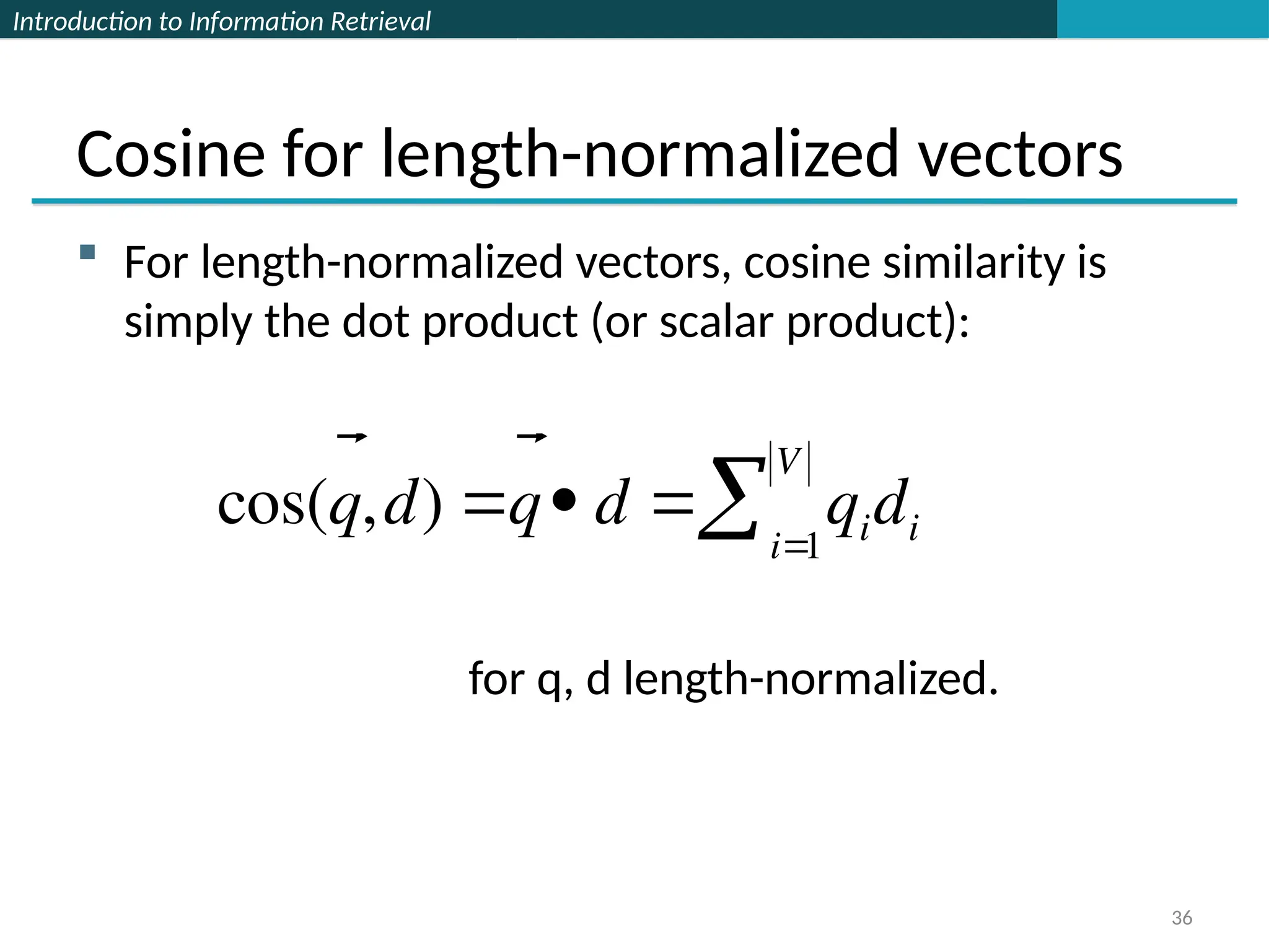
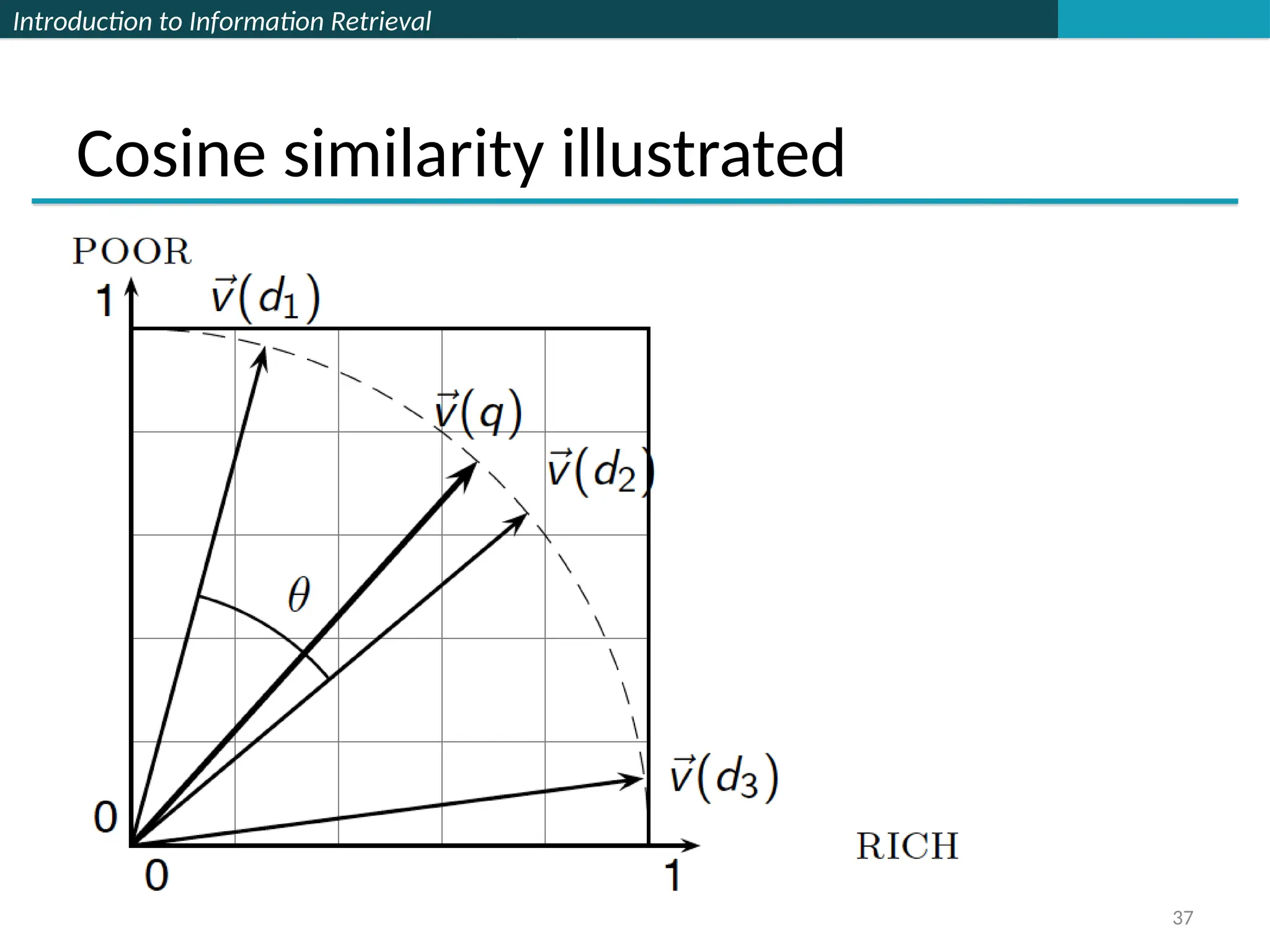
From angles to cosines
 The following two notions are equivalent.
 Rank documents in decreasing order of the angle between
query and document
 Rank documents in increasing order of
cosine(query,document)
 Cosine is a monotonically decreasing function for the
interval [0o
, 180o
]
Sec. 6.3

33. Introduction to Information Retrieval
From angles to cosines
 But how – and why – should we be computing cosines?
Sec. 6.3

34. Introduction to Information Retrieval
Length normalization
 A vector can be (length-) normalized by dividing each
of its components by its length – for this we use the
L2 norm:
 Dividing a vector by its L2 norm makes it a unit
(length) vector (on surface of unit hypersphere)
 Effect on the two documents d and d (d appended to
′
itself) from earlier slide: they have identical vectors
after length-normalization.
 Long and short documents now have comparable weights

 i i
x
x 2
2

Sec. 6.3

35. Introduction to Information Retrieval
cosine(query,document)











V
i i
V
i i
V
i i
i
d
q
d
q
d
d
q
q
d
q
d
q
d
q
1
2
1
2
1
)
,
cos( 









Dot product Unit vectors
qi is the tf-idf weight of term i in the query
di is the tf-idf weight of term i in the document
cos(q,d) is the cosine similarity of q and d … or,
equivalently, the cosine of the angle between q and d.
Sec. 6.3

36. Introduction to Information Retrieval
Cosine for length-normalized vectors
 For length-normalized vectors, cosine similarity is
simply the dot product (or scalar product):
for q, d length-normalized.
36


cos(

q,

d) 

q 

d  qidi
i
1
V


37. Introduction to Information Retrieval
Cosine similarity illustrated
37

38. Introduction to Information Retrieval
Cosine similarity amongst 3 documents
term SaS PaP WH
affection 115 58 20
jealous 10 7 11
gossip 2 0 6
wuthering 0 0 38
How similar are
the novels
SaS: Sense and
Sensibility
PaP: Pride and
Prejudice, and
WH: Wuthering
Heights?
Term frequencies (counts)
Sec. 6.3
Note: To simplify this example, we don’t do idf weighting.

39. Introduction to Information Retrieval
3 documents example contd.
Log frequency weighting
term SaS PaP WH
affection 3.06 2.76 2.30
jealous 2.00 1.85 2.04
gossip 1.30 0 1.78
wuthering 0 0 2.58
After length normalization
term SaS PaP WH
affection 0.789 0.832 0.524
jealous 0.515 0.555 0.465
gossip 0.335 0 0.405
wuthering 0 0 0.588
cos(SaS,PaP) ≈
0.789 × 0.832 + 0.515 × 0.555 + 0.335 × 0.0 + 0.0 × 0.0
≈ 0.94
cos(SaS,WH) ≈ 0.79
cos(PaP,WH) ≈ 0.69
Why do we have cos(SaS,PaP) > cos(SaS,WH)?
Sec. 6.3

40. Introduction to Information Retrieval
Computing cosine scores
Sec. 6.3

41. Introduction to Information Retrieval
tf-idf weighting has many variants
Columns headed ‘n’ are acronyms for weight schemes.
Why is the base of the log in idf immaterial?
Sec. 6.4

42. Introduction to Information Retrieval
Weighting may differ in queries vs
documents
 Many search engines allow for different weightings
for queries vs. documents
 SMART Notation: denotes the combination in use in
an engine, with the notation ddd.qqq, using the
acronyms from the previous table
 A very standard weighting scheme is: lnc.ltc
 Document: logarithmic tf (l as first character), no idf
and cosine normalization
 Query: logarithmic tf (l in leftmost column), idf (t in
second column), no normalization …
A bad idea?
Sec. 6.4

43. Introduction to Information Retrieval
tf-idf example: lnc.ltc
Term Query Document Prod
tf-
raw
tf-wt df idf wt n’lize tf-raw tf-wt wt n’lize
auto 0 0 5000 2.3 0 0 1 1 1 0.52 0
best 1 1 50000 1.3 1.3 0.34 0 0 0 0 0
car 1 1 10000 2.0 2.0 0.52 1 1 1 0.52 0.27
insurance 1 1 1000 3.0 3.0 0.78 2 1.3 1.3 0.68 0.53
Document: car insurance auto insurance
Query: best car insurance
Exercise: what is N, the number of docs?
Score = 0+0+0.27+0.53 = 0.8
Doc length = 12
 02
12
1.32
1.92
Sec. 6.4

44. Introduction to Information Retrieval
Summary – vector space ranking
 Represent the query as a weighted tf-idf vector
 Represent each document as a weighted tf-idf vector
 Compute the cosine similarity score for the query
vector and each document vector
 Rank documents with respect to the query by score
 Return the top K (e.g., K = 10) to the user

45. Introduction to Information Retrieval
Resources for today’s lecture
 IIR 6.2 – 6.4.3
 http://www.miislita.com/information-retrieval-tutori
al/cosine-similarity-tutorial.html
 Term weighting and cosine similarity tutorial for SEO folk!
Ch. 6