SlideShare a Scribd company logo
1 of 67
Biostatistics and Computer Application
M.Sc. Biotechnology
(MSBT-109- DTU)
Unit I
Fundamental of probability
Hypothesis testing
Unit II
Database Management
Introduction to
programming language
Unit III
Cluster analysis
Unit IV
Microarray technique
Spectroscopy for
protein structure
Unit V
Modelling Methods
• Homology Modelling
• Protein str. Prediction
• Parameters: Force filed,
Gibbs energy, Monte
Carlo,energy minimization
and simulation/docking
• RNA expression studies
• Data normalization
• Differential expression of
genes- threshold p- values
• Introduction to X-ray
crystallography and NMR
spectroscopy
• Protein structure database &
visualization
• Phylogeny clustering
• Pattern recognition methods
• Sequence analysis
• protein family classification
examples
• Types of databases
• Data retrieval & browsing
• Databases like PubMed,
NCBI, UCSC, EMBL
browsing
• Central limit theorem- normal
distribution
• Discrete & continuous
variables
• Confidence interval & levels
of significance & critical
region • Basics of programming
language
• Application of language in
biostatistics
• Null & alternate hypothesis
• Statistical test: p- value
✔ Student T test
✔ Z test – Fischer test
✔ ANOVA- one way or two way
• Application of statistical tests
in research studies
CLASS-I
16 Aug 2023
What is Statistics
Statistics is the area of applied math that deals with the collection, organization, analysis, interpretation, and
presentation of data.
Biostatistics is the application of statistical techniques to scientific research in health-related fields, including
medicine, biology, and public health.
Two main branches of Statistics:
• Descriptive Statistics
• Inferential Statistics
Descriptive statistics focus on describing the visible characteristics of a dataset. A data set is a collection of
responses or observations from a sample or entire population. They represent all of the procedures that can be
used to organise, summarise, display, and categorise data collected for a certain experiment or event. It
includes tabulation, graphical presentation, measures of central tendency, etc
Inferential statistics focus on making predictions or generalizations about a larger dataset, based on a
sample of those data. The inferential statistics include z test, t test, analysis of variance, etc.
In short statistics are about summarizing and answering question based on data.
A measurement or datum is a single observation. Data (plural) are a collection of scores.
Descriptive statistics
• Describe the features of populations and/or samples
• Organize and present data in a purely factual way
• Present final results visually, using tables, charts, or graphs
• Draw conclusions based on known data
• Use measures like central tendency, distribution, and variance
Descriptive Statistics
Descriptive Statistics are used to summarize, organize and simplify data
Descriptive Statistics
Inferential statistics
Use samples to make generalizations about larger populations
Help us to make estimates and predict future outcomes
Present final results in the form of probabilities
Draw conclusions that go beyond the available data
Use techniques like hypothesis testing, confidence intervals, and
regression and correlation analysis
Inferential Statistics
• The population may be defined as the entire number of observations that constitute a particular group.
Samples are generally a relatively small group of observations that have been taken from a defined
population.
• Parameters are characteristics of populations while statistic are characteristics of samples representing
summary measures computed on observed sample values.
• Parameters or population values are usually represented by Greek symbols (e.g. μ) and sample statistic
are denoted by letters (e.g. x
̄ )
Population and Samples
Ques: what’s the mean diastolic blood pressure of the given population?
Sampling error: The discrepancy
between the sample statistic and
the true population parameter it is
estimating.
To reduce the sampling error:
✔ Sufficiently large sample size
✔ Random selection (unbiased
sample collection)
⮚ Problem Solving
⮚ Use in Clinical Trials
⮚ Use in Manufacturing of Pharmaceuticals
⮚ Use in Quality Control of Pharmaceuticals
⮚ Use in Research and Development of Drugs and Technology
⮚ Use in Anatomy and Physiology
⮚ Use in Pharmacology and Medicine
⮚ Use in Community Medicine and Public Health
⮚ Use in Health and Vital statistics
⮚ Use in Biotechnology, Bioinformatics and Computational Biotechnology
Applications and Uses of Biostatistics
Variables and Constants
✔ A constant is a characteristic that is fixed across conditions. For example: fingerprint, country in which you
were born, genotype.
✔ A variable is something that changes across conditions. For example salary, age, marital status, respiratory
rate, blood type etc. Data are the values we get when we measure or observe a variable.
✔ How do we measure things?
Qualitatively: By putting them into categories
Quantitatively: By using numbers
A typical characteristics of this variable are that they do not have any units of measurement, and the ordering
of the categories is completely arbitrary. Example: Blood group types - Nominal categorical variable
This data too do not have any units of measurement as like that of nominal variables but the ordering of the
categories is not arbitrary as it was with nominal variables. Example: Scoring of a patients- Ordinal
Ordinal data are not real numbers. They cannot be placed on the number line. As ordinal data are not real
numbers, it is not appropriate to apply any of the rules of basic arithmetic to sort this data
Nominal
Variable
Continuous
Variable
With metric variables, proper measurement is possible and therefore these variables produce data that are real
numbers, and can be placed on the number line.
Metric continuous variables can be properly measured and have units of measurement. Example: Birth weight
(g), blood pressure (mmHg)- Metric continuous
Continuous metric data usually comes from measuring while discrete metric data, usually comes from counting
The data produced are real numbers, and are invariably integer (i.e. whole number). They can be placed on the
number line, and have the same interval and ratio properties as continuous metric data.
Metric discrete variables can be properly counted and have units of measurement- ‘numbers of things’.
Example: Number of deaths, number of pressure sores, number of angina Attacks- discrete variables
Discrete
Variable
Ordinal
Variable
Variables
Identify type of variable:
1. Dosage form - tablet/ capsule / ointment
2. Bioavailability measurements (C ,T ,AUC)
3. Age ( in years).
4. Hypertension -Mild, Moderate and Severe
5. Smoking history (cigarattes per day)
6. Test- pass or fail criteria
7. Weight
8. Male vs female subjects
9. Scores for patient responses to treatment
Summary
1. Biostatistics is branch of statistics applied to_______ science whereby collection, classification, summarising, analysis and
interpretation of data is done. a. pharmaceutical b. medicinal c. biological d. chemical
2. Descriptive statistics represents all of the procedures that can be used to_______.
a. organise, summarise
b. display and categorise
c. a & b
d. none of above
3. The population is_________. a. the entire number of observations that constitutes a particular group. b. the entire number of samples
that constitutes a particular group. c. a & b d. None of above
4. Categorical variable can be divided into__________. a. Nominal & continuous b. nominal & discrete c. discrete&continuous d.
nominal&ordinal
5. Metric data can be divided into___________. a. Nominal & continuous b. nominal & discrete c. discrete&continuous d.
nominal&ordinal
6. The goal of ___________ is to focus on summarizing and explaining a specific set of data. a. inferential statistics b. descriptive
statistics c. none of the above d. all of the above
7. Metric variable can be properly_________. a. measured b. counted c. a & b d. none of the above
8. In categorical variables, values are in ________ categories. a. arbitrary & counted b. arbitrary & measured c. arbitrary & ordered d.
counted & measured.
9. Bioavailability measurement is a ___________ variable. a. metric continuous b. metric discrete c. categorical continuous d.
categorical ordinal.
10. Scores for patient responses to treatment is a ____________ variable. a. metric continuous b. metric discrete c. categorical
continuous d. categorical ordinal
Fundamental of Biostatistics- Basic concepts and terminologies
Gender
Eye Color
Identify type of variable:
Ethnicity
Places in a Race
Olympics medals
Cloth sizes
CLASS-II
18 Aug 2023
01 02 04
03
Frequency
Distribution
Graphical
representations
Shape of data
distribution
Central tendency and
dispersion
Learning objectives
Fundamental of Biostatistics- Data Representation and Distribution
▪ Whenever the data is collected for some project, it is usually in the ‘raw’ form and not in a organised way.
▪ Descriptive statistics deals with sorting this raw data by putting it into a table or by presenting it in an appropriate chart or
summarising it numerically.
▪ An important consideration in sorting the raw data is the type of variable concerned. The data from some variables are best
described with a table, some with a chart, and some with both. However, a numeric summary is more appropriate for some types
of variable
▪ Tabulation is the first step before the data is used for analysis or interpretation.
▪ Frequency distribution tables presents data in a relatively compact form, ready to use but certain information may be lost. The
data can be reduced to manageable form using frequency tables. It can have one or all the following parameters, depending on the
type of data.
1. Frequency tells you how often something happened OR number of times that any particular value come in a data.
2. Relative frequency is the frequency converted into percentage of the total number of observations.
3. Cumulative frequency is the cumulative total of frequencies and is obtained by adding the frequency of observations at each
level point to those frequencies of the preceding level(s).
4. Cumulative relative frequency It is cumulative frequency converted into the percentage of the total number of observations.
⮚ Frequency distribution in nominal data
Shows that a higher percentage of nurses than of doctors work
in rural areas, but that, overall, a greater proportion of staff
works in urban areas (67%).
⮚ It makes no sense to calculate cumulative frequency for nominal data, because of the arbitrary category order.
Hence, cumulative frequency is not calculated. But can be done for the ordinal data.
The Cumulative and relative cumulative
frequency distributions for data
Frequency tables can show either categorical variables (sometimes called qualitative variables) or quantitative variables
(numeric values).
Relative frequency table showing the percentage of
students in each blood group
⮚ The most useful approach with metric continuous data is to group them first, and then construct a frequency
distribution of the grouped data.
It requires major components: class, class limits, boundaries and intervals. Also class marks and open ended
groups can be used.
• Class: (range of data points) ÷ (range of classes) eg 20 ÷ 5 = 4
• Class size: Difference between the lower and upper class-limits.
• Class limit: Represent the smallest and largest data values that can belong to each class.
• Class interval: Difference between the upper and lower class limit
• Classmark : Average of the upper and lower limits of a class.
The frequency distribution table for metric discrete data
The relative, cumulative and relative cumulative frequency distribution table
⮚ Grouped frequency table:
Exclusive Class Interval: the upper limit of one class is the same as the lower limit of the
succeeding class. Note that in continuous cases, any observation corresponding to the
extreme values of a class is always included in that class where it is the lower limit. For
example, if we had a student who has scored 5 marks in the test, his marks would be
included in the class interval 5-10 and not 0-5.
Inclusive Class interval: the lower limit of a class does not get repeated in the upper limit
of the preceding class. When a frequency distribution is analyzed the iinclusive class
interval has to be converted to an exclusive class interval. This can be done by subtracting
0.5 from the lower class limit and adding 0.5 to the upper class limit.
Practice question
Construct a frequency table for the data on marks obtained by 20 students in their math exam.
20,43,74,89,75,60,31,43,37,36,50,38,21,99,93,45,64,92,38,60
Class Freq Relative freq Cumulative freq Relative Cumulative
freq
20-40
40-60
60-80
80-100
⮚ Graphical presentation of data with appropriate chart is a good idea for describing data effectively. Appropriate chart depends primarily on the type of data, as
well as on what particular features of it we are looking for.
✔ The Graphical Presentation of Data
1. Pie chart is a diagram in which the frequencies of the groups are shown in a circle. Each
segment (slice) of a pie chart should be proportional to the frequency of the category it
represents. A disadvantage of a pie chart is that it can only represent one variable. It can lose
clarity if it is used to represent more than four or five categories
Pie chart of percentage
blood group of pharmacy
students
Simple bar chart of blood
group of pharmacy students
Clustered bar chart of blood group of 95 pharmacy students by sex
A stacked bar chart of blood group of
95 pharmacy students by sex
2. Bar chart: Its a chart with frequency on the vertical axis and category on the horizontal axis.
The simple bar chart is appropriate if only one variable is to be shown.
All the bars should be of the same width, and there should be equal spaces between bars.
These spaces emphasise the categorical nature of the data
3. Clustered bar chart: If there are more than one group, we can use the clustered bar chart.
There are two ways of presenting a clustered bar chart. As it compare the relative sizes of
the groups within each category.
4. Stacked bar charts: The bars are now stacked on top of each other. Stacked bar charts
are appropriate if we want to compare the total number of subjects in each group but
not so good if we want to compare category sizes between groups.
5. Pictograms are similar to bar charts. They present
the same type of information, but the bars are
replaced with a proportional number of icons. This
type of presentation for descriptive statistics dates
back to the beginning of civilization when pictorial
images were used to record numbers of people,
animals or objects.
Population of different districts of Western
Maharashtra. Each diagram indicates one lakh
6. Line chart is similar to a bar chart except that thin lines, instead of thicker bars, are
used to represent the frequency associated with each level of the discrete variable
7. Point plots are identical to line charts, however, instead of a line, a number of points or
dots equivalent to the frequency are stacked vertically for each value of the horizontal
axis. Also referred to as dot diagram, point plots are useful for small data sets.
Line and Point Plot of assay result of 30 amoxicillin tablets
8. A histogram looks like a bar chart but without any gaps between adjacent bars. This
emphasises the continuous nature of the underlying variable.
- If the groups in the frequency table are all of the same width, then the bars in the
histogram will also be of the same width.
- One limitation of the histogram is that it can represent only one variable at a time (like the
pie chart), and this can make comparisons between two histograms difficult.
histogram of the grouped weight in kg
9. A frequency polygon can be constructed by placing a dot at the midpoint (class mark) for
each class interval in the histogram and then these dots are connected by straight lines.
- This frequency polygon gives a better conception of the shape of the distribution. The
class interval midpoint for a section in a histogram is calculated as follows: Midpoint =
(highest + lowest point)/2
- The frequency polygon is then created by listing the midpoints (class marks) on the x
axis, frequencies on the y-axis, and drawing lines to connect the midpoints for each
interval.
A Frequency Polygon of the grouped weight in kg
Ogive of the grouped weight of
60 final year students
10. Relative Cumulative Frequency Curve (Ogive) is a graph of the cumulative relative frequency distribution.
⮚ So, to draw Ogive we should convert ordinary frequency distribution into relative cumulative frequency.
⮚ With continuous metric data, there is assumed to be a smooth continuum of values, so we can chart relative cumulative frequency with a correspondingly smooth curve, or ogive.
✔ By using Ogive we can locate any percentile that will divide the series into parts.
▪ Quartiles: There are three different points located on the entire range of variable. By using these quartiles we can
calculate semi inter quartile range and inter quartile range (Q1-Q3).
- Q1 or lower quartile will have 25% observations falling in its left and 75% observations on its right side.
- Q2 is the median, i.e.,50%values lies on either side.
- Q3 is the upper quartile, will have 75% observations falling on its left side and 25% observations on its right side.
▪ Deciles: This divides the distribution into 10 equal parts. First decile
(10th percentile) will have 10% values to its left and 90% values to
its right. 5th decile is the median and contains 50% values on either
side.
▪ Quintiles: This divides the distribution into 5 equal parts. So, 20th
percentile or 1st quintile will have 20% observations falling to its
left and 80% to its right.
CLASS-III
23 Aug 2023
12. The stem-and-leaf plot is a visual representation for continuous data and contains features
common to both the frequency distribution and dot diagrams. Digits, instead of bars are used to
illustrate the spread and shape of the distribution. Each piece of data is divided into "leading" and
"trailing" digits.
All the leading digits are sorted from lowest to highest and listed to the left of a vertical line. These
digits become the stem. The trailing digits are then written in the appropriate location to the right of
the vertical line. These become the leaves.
11. Box-whisker plot: This plot that displays a great deal of information about a continuous variable
is the box-and-whisker plot. It shows the bulk of the data as a rectangular box in which the upper
and lower lines represent the third quartile (75% of observations below Q3) and first quartile (25%
of observations below Ql), respectively. The second quartile (50% of the observations below this
point) is depicted as a horizontal line through the box. Vertical lines (whiskers) extend from the top
and bottom lines of the box to an upper and lower adjacent value.
13. A scatter diagram is an extremely useful presentation for showing the relationship between two
continuous variables. The two dimensional plot has both horizontal and vertical axes which cover
the ranges of the two variables. Plotted data points represent paired observations for both the x and
y variable. These types of plots are valuable for correlation and regression inferential tests.
14. Time series plot: If the data collected are from
measurements made at regular intervals of time
(minutes, weeks, years, etc.), we can present the
data with a time series chart. Usually these
charts are used with metric data, but may also be
appropriate for ordinal data. Time is always
plotted on the horizontal axis, and data values on
the vertical axis.
1. The values are fairly evenly spread
throughout their possible range. This
is a uniform distribution.
2. The values are concentrated towards the
bottom of the range, with progressively
fewer values towards the top of the range.
This is a right or positively skewed
distribution.
3. The values are concentrated towards the top
of the range, with progressively fewer values
towards the bottom of the range. This is a left
or negatively skewed distribution.
4. The values are clumped together around one
particular value, with progressively fewer
values both below and above this value. This is
a symmetric or mound-shaped distribution.
5. The values are clumped around two or
more particular values. This is a
bimodal or multimodal distribution.
✔ There is one particular symmetric bell-shaped
distribution, known as the Normal distribution. Many
human clinical features are distributed normally
The choice of the most appropriate procedures for summarising and analysing data will not only depend on the type of variable but also on the shape of the
distribution.
Fundamental of Biostatistics- Data Distribution
✔ It is bell shaped curve
✔ It is symmetrical in distribution; variables on either side of mean are equal in
number.
✔ Its maximum height is at the mean.
✔ Mean= mode= median , in case of normal distribution coincide.
✔ Skewness of the curve is zero.
✔ It is asymptotic, in that tails never touch baseline.
✔ Total area of curve is one and standard deviation is also one.
✔ It has two curves. Central part is convex and when it comes down, it becomes
concave on both sides.
Skewness measures asymmetry around the mean. The parameter is best interpreted as
relative to the normal distribution (whose skewness equals to zero).
The interpretation of the skewness is :
⮚ Skewness > 0 asymmetric tail with more values above the mean
⮚ Skewness < 0 asymmetric tail with more values below the mean
Skewed data is required to be treated using non parametric tests while normal curve
data is treated using parametric tests.
Kurtosis is a property associated with a frequency distribution and refers to the shape
of the distribution of values regarding its relative flatness and peaked-ness. Compared
with normal distribution, the interpretation of the kurtosis is:
⮚ Kurtosis > 0 peaked relative to Normal distribution
⮚ Kurtosis < 0 flat relative to Normal distribution
⮚ In any research, enormous data is collected and, to describe it
meaningfully, one needs to summarise the same.
⮚ The bulkiness of the data can be reduced by organising it into a
frequency table or histogram.
⮚ Frequency distribution organises the heap of data into a few meaningful
categories.
⮚ Collected data can also be summarised as a single index/value, which
represents the entire data.
⮚ These measures may also help in the comparison of data.
✔ Defined as “the statistical measure that identifies a single value as
representative of an entire distribution”.
✔ It aims to provide an accurate description of the entire data.
✔ It is the single value that is most typical/representative of the collected data.
Mean is generally considered the best measure of central tendency and the
most frequently used.
However, there are some situations where the other measures of central
tendency are preferred.
✔ The mean, median and mode are the three commonly used measures of
central tendency.
Measure of Central
Tendency
❑ Arithmetic mean (or, simply, “mean”) is nothing but the average. It is computed by adding all the values in the data set divided by the number of
observations in it.
Measure of Central Tendency- Types of Averages
❑ Median is the value which occupies the middle position when all the observations are arranged in an ascending/descending order. It divides the
frequency distribution exactly into two halves. 50% of observations in a distribution have scores at or below the median. Hence median is the 50th
percentile. Median is also known as ‘positional average’.
❑ Mode is defined as the value that occurs most frequently in the data. Some data sets do not have a mode because each value occurs only once. On the
other hand, some data sets can have more than one mode. This happens when the data set has two or more values of equal frequency which is greater than
that of any other value. Mode is rarely used as a summary statistic except to describe a bimodal distribution. In a bimodal distribution, the taller peak is
called the major mode and the shorter one is the minor mode.
Median is preferred to mean when:
✔ There are few extreme scores in the distribution.
✔ Some scores have undetermined values.
✔ There is an open ended distribution.
✔ Data are measured in an ordinal scale.
⮚ Mode is the preferred measure when data are measured in a nominal scale.
Measuring dispersion or variations associated with Central Tendency
1. The range is the distance from the smallest value to the largest. Not affected by skewness, but is sensitive to the addition or
removal of an outlier value. Range = Lowest value to Highest value.
2. The interquartile range describes the middle 50% of values when ordered from lowest to highest. To find the interquartile
range (IQR), ​first find the median (middle value) of the lower and upper half of the data. These values are quartile 1 (Q1)
and quartile 3 (Q3). The IQR is the difference between Q3 and Q1. It is not affected either by outliers or skewness, but it
does not use all of the information in the data set since it ignores the bottom and top quarter of values.
3. Standard Deviation is a measure which shows how much variation (such as spread, dispersion, spread,) from the mean exists. It indicates a “typical” deviation
from the mean. The most widely used measure of dispersion, is based on all values. It is the square root, of the, mean of the squared deviations, from arithmetic
mean. In statistics, Variance and standard deviation are related with each other since the square root of variance is considered the standard deviation for the given
data set.
4. The mean deviation is defined as a statistical measure that is used to calculate the
average deviation from the mean value of the given data set. It uses absolute
values instead of squares to circumvent the issue of negative differences between
the data points and their means.
Population Parameters versus Sample Statistics
Biostatistics is to analyze samples in order to make inferences about the population from which the samples were drawn
s2 = 472.10/9 = 52.46 s = √52.46 = 7.24
Which statistics should be used to describe the distribution below?
a. Mean and IQR
b. Mean and Standard Deviation
c. Median and IQR
d. Median and Standard Deviation
Q: Salary (in K) of students after PG
35, 50,50,50,56,60,60,75,250
Mean= ~76.2 and SD = ~ 62.3
Median=56 and IQR=17.5
Questions
CLASS-IV
25 Aug 2023
Probability and its fundamental concepts related to biostatistics
⮚ The probability is the likelihood of occurrence of a particular event or chance of
occurrence for an event.
⮚ Experiment refers to describe an act which can be repeated under some given
conditions. Those experiments whose results depends on chance are called random
experiment. Outcomes of an any experiment are called EVENTS.
⮚ Mutually exclusive events: (Incompatible) When two events cannot happen
simultaneously in a single trail. Basically, occurrence of any one event precludes
the occurrence of another events.
(A AND B) = P(AՈB)
(A OR B) = P(AUB)
Playing with cards
How many cards we have in a Deck ?
1. A card is drawn from a well shuffled pack of 52
cards. Find the probability of:
(i) ‘2’ of spades
(ii) a jack
(iii) a king of red colour
(iv) a card of diamond
(v) a king or a queen
(vi) a non-face card
(vii) a black face card
(viii) a black card
(ix) a non-ace
(x) non-face card of black colour
(xi) neither a spade nor a jack
(xii) neither a heart nor a red king
2. A card is drawn at random from a well-shuffled
pack of cards numbered 1 to 20. Find the
probability of
(i) getting a number less than 7
(ii) getting a number divisible by 3.
3. A card is drawn at random from a pack of 52
playing cards. Find the probability that the card
drawn is
(i) a king
(ii) neither a queen nor a jack.
⮚ Independent events: Two or more events are said to be
independent, when the outcome of one event is not affected
by other outcomes, as they do not effect other.
⮚ Eg. If a coin is tossed twice, the result of second throw is
not affected by the result of the first throw.
✔ Single-event: we consider, probability of
happening or not happening of single events.
It deals with elementary events.
✔ Compound-event: we consider, the joint
occurrence of two or more events. It deals
with composite events.
✔ Exhaustive-event: Those events whose
totality includes all possible outcomes of
RANDOM experiment or sample space.
✔ Complementary-event: Let A & B are
two events and both of them are
mutually exclusive and exhaustive
events. Then A is complementary event
of B (& VICE-VERSA).
⮚ Dependent events: In these events occurrence or non-
occurrence of one event in any one trial affects the
probability of other events in other trails.
⮚ Equally likely event are said to be equally likely when
one does not occur more often than the others.
(A AND B) = P(AՈB)
(A OR B) = P(AUB)
CLASS-V
30 Aug 2023
None of the students
attended the class
CLASS-VI
1st September 2023
Probability Distributions
Experiment, Outcome, and Sample Space
An experiment is a process that, when performed, results in one and only one of many observations. These observations are called the
outcomes of the experiment. The collection of all outcomes for an experiment is called a sample space.
Examples of Experiments, Outcomes, and Sample Spaces Tree diagram, each outcome is represented by a branch of the
tree.
• help us understand probability concepts by presenting them
visually
⮚ tree diagram for the experiment of tossing a coin once
Sample space = {H, T}, where H = Head and T = Tail
⮚ Suppose we randomly select two workers from a company
and observe whether the worker selected each time is a man or
a woman.
Sample space = {MM, MW, WM, WW}
Tree diagram for
one toss of a coin.
Simple and Compound Events
An event is a collection of one or more of the outcomes of an experiment.
A simple event is also called an elementary event, and a compound event is also called a composite event.
Simple Event An event that includes one and only one of the (final) outcomes for an experiment is called a simple event and is
usually denoted by Ei.
Reconsider previous example: on selecting two workers from a company and observing whether the worker selected each time is a
man or a woman.
Each of the final four outcomes (MM, MW, WM, and WW) for this experiment is a simple event.
These four events can be denoted by E1, E2, E3, and E4, respectively.
Thus, E1 = {MM}, E2 = {MW}, E3 = {WM}, and E4 = {WW}
Compound Event A compound event is a collection of more than one outcome for an experiment.
Reconsider the same example on selecting two workers from a company and observing whether the worker selected each time is a man
or a woman. Let A be the event that at most one man is selected. Is event A a simple or a compound event?
Here at most one man means one or no man is selected.
Thus, event A will occur if either no man or one man is selected.
Hence, the event A is given by
A = at most one man is selected = {MW, WM, WW}
Because event A contains more than one outcome, it is a compound event.
Q: In a group of college students, some like ice tea and others do not. There is no student in this
group who is indifferent or has no opinion. Two students are randomly selected from this group.
(a) How many outcomes are possible? List all the possible outcomes.
(b) Consider the following events. List all the outcomes included in each of these events.
Mention whether each of these events is a simple or a compound event.
(i) Both students like ice tea.
(ii) At most one student likes ice tea.
(iii) At least one student likes ice tea.
(iv) Neither student likes ice tea.
Let L denote the event that a student likes ice tea and N
denote the event that a student does not like ice tea.
(a) This experiment has four outcomes,
LL = Both students like ice tea
L N = The first student likes ice tea but the second student
does not
NL = The first student does not like ice tea but the second
student does
NN = Both students do not like ice tea
(b) (i) The event both students like ice tea will occur if LL happens.
Thus, Both students like ice tea = {L L}
Since this event includes only one of the four outcomes, it is a simple event.
(ii) The event at most one student likes ice tea will occur if one or none of the
two students likes ice tea.
At most one student likes ice tea = {L N, NL, N N}
Since this event includes three outcomes, it is a compound event.
(iii) The event at least one student likes ice tea will occur if one or two of the
two students like ice tea.
Thus, At least one student likes ice tea = {LN, NL, LL}
Since this event includes three outcomes, it is a compound event.
(iv) The event neither student likes ice tea will occur if neither of the two
students likes ice tea, which will include the event NN.
Thus, Neither student likes ice tea = {NN}
Since this event includes one outcome, it is a simple event.
Probability is a numerical measure of the likelihood that a specific event will occur. The probability that a simple event Ei will occur is
denoted by P(Ei), and the probability that a compound event A will occur is denoted by P(A).
Two Properties of Probability
1. The probability of an event always lies in the range 0 to 1.
Whether it is a simple or a compound event, the probability of an event is never less than 0 or greater than 1.
0 ≤ P(Ei) ≤ 1
0 ≤ P(A) ≤ 1
2. The sum of the probabilities of all simple events (or final outcomes) for an experiment, denoted by ΣP(Ei), is always 1.
For an experiment with outcomes E1, E2, E3, .a . . ,
ΣP(Ei) = P(E1) + P(E2) + P(E3) + . . . = 1.0
Classical Probability: Equally Likely Outcomes Two or more outcomes that have the same probability of occurrence are said to be
equally likely outcomes.
Marginal probability is the probability of a single event without consideration of any other event.
Example: 15 employees in this group possess two characteristics: “male” and “in favor of paying high salaries to CEOs.”
Suppose one employee is selected at random from these 100 employees. If only one characteristic is considered at a time, the
employee selected can be a male, a female, in favor, or against. The probability of each of these four characteristics or events is
called marginal probability.
The four marginal probabilities are calculated as follows:
P(male) = Number of males/ Total number of employees = 60/100 = .60
As we can observe, the probability that a male will be selected is
obtained by dividing the total of the row labeled “Male” (60) by the
grand total (100). Similarly,
P(female) = 40/100 = .40
P(in favor) = 19/100 = .19
P(against) = 81/100 = .81
Now suppose that one employee is selected at random from these 100 employees. Furthermore, assume it is
known that this (selected) employee is a male. In other words, the event that the employee selected is a male
has already occurred. Given that this selected employee is a male, he can be in favor or against. What is the
probability that the employee selected is in favor of paying high salaries to CEOs?
Conditional probability is the probability that an event will occur given that another event has already occurred. If A
and B are two events, then the conditional probability of A given B is written as P(A ∣ B)
and read as “the probability of A given that B has already occurred.”
Mutually Exclusive Events : Events that cannot occur together are said to be mutually exclusive events.
Consider the following events for one roll of a die:
A = an even number is observed = {2, 4, 6}
B = an odd number is observed = {1, 3, 5}
C = a number less than 5 is observed = {1, 2, 3, 4}
Are events A and B mutually exclusive? Are events A and C mutually exclusive?
Independent Events Two events are said to be independent if the occurrence of one event does not affect the probability of the
occurrence of the other event. In other words, A and B are independent events if either P(A ∣ B) = P(A) or P(B ∣ A) = P(B)
Complementary Events: The complement of event A, denoted by A and read as “A bar” or “A complement,” is the event that
includes all the outcomes for an experiment that are not in A.
Events A and A are complements of each other.
Because two complementary events, taken together, include all the outcomes for an experiment and
because the sum of the probabilities of all outcomes is 1, it is obvious that
P(A) + P(A) = 1.0
Question: Of the 500 adults, 325 drink coffee with sugar.
Suppose one adult is randomly selected from these 500
adults, and let A be the event that this adult drinks coffee
with sugar. What is the complement of event A? What are
the probabilities of the two events?
Mutually exclusive events A
and B.
Mutually nonexclusive
events A and C.
Theorem of probability
Joint Probability The probability of the intersection of
two events is called their joint probability.
It is written as P(A and B)
Union of Events : Let A and B be two events defined in a sample space. The union of events A and B is the collection of
all outcomes that belong either to A or to B or to both A and B and is
denoted by (A or B); (A ∪ B)
Counting Rule: to Find Total Outcomes If an experiment consists of three steps, and if the first step can result in m
outcomes, the second step in n outcomes, and the third step in k outcomes, then
Total outcomes for the experiment = m · n · k
The symbol ! (read as factorial) is used to denote factorials. The value of the factorial of a numberis obtained by
multiplying all the integers from that number to 1. For example, 7! is read as “seven factorial” and is evaluated
by multiplying all the integers from 7 to 1.
Example: Evaluate 7!.
Solution To evaluate 7!, we multiply all the
integers from 7 to 1.
7!= 7 ⋅ 6 ⋅ 5 ⋅ 4 ⋅ 3 ⋅ 2 ⋅ 1 = 5040
Thus, the value of 7! is 5040.
Example: Consider three tosses of a coin. How many total outcomes this experiment has?
Solution This experiment of tossing a coin three times. Each step has two outcomes: a head and a tail. Thus,
Total outcomes for three tosses of a coin = 2 × 2 × 2 = 8
The eight outcomes for this experiment are HHH, HHT, HTH, HTT, THH, THT, TTH, and TTT.
Counting Rule, Factorials
Discrete Random Variables and Their Probability Distributions
Random Variable: A random variable is a variable whose value is determined by the outcome of a random experiment.
Discrete Random Variable A random variable that assumes countable values is called a discrete random variable.
examples of discrete random variables
• The number of houses in a certain block
• The number of customers who visit a bank during any given hour
• The number of complaints received at the office of an airline on a given day
Continuous Random Variable A random variable that can assume any value contained in one or more intervals is called
a continuous random variable.
Examples of continuous random variables
• The length of a room
• The time taken to commute from home to work
• The weight of a letter
• The price of a house
Probability Distribution of a Discrete Random Variable:
⮚ Binomial Probability Distribution
⮚ Poisson Probability Distribution
⮚ Hypergeometric Probability Distribution
The Binomial Probability Distribution
✔ most widely used discrete probability distributions.
✔ the random variable x must be a discrete dichotomous random variable.
✔ Each repetition of a binomial experiment is called a trial or a Bernoulli trial.
✔ For example, if an experiment is defined as one toss of a coin and this experiment is repeated 10 times, then
each repetition (toss) is called a trial. Consequently, there are 10 total trials for this experiment.
An experiment that satisfies the following four conditions is called a binomial experiment.
1. There are n identical trials. In other words, the given experiment is repeated n times, where n is a positive integer. All of these
repetitions are performed under identical conditions.
2. Each trial has two and only two outcomes. These outcomes are usually called a success and a failure, respectively. In case there are
more than two outcomes for an experiment, we can combine outcomes into two events and then apply binomial probability
distribution.
3. The probability of success is denoted by p and that of failure by q, and p + q = 1. The probabilities p and q remain constant for each
trial.
4. The trials are independent. In other words, the outcome of one trial does not affect the outcome of another trial.
Note: Success does not mean favorable or desirable outcome and a failure does not refer to an unfavorable or undesirable outcome.
The outcome to which the question refers is usually called a success; the outcome to which it does not refer is called a failure.
n = total number of trials = number of students selected = 3
x = number of successes = number of students in three who use Instagram = 2
p = probability of success = probability that a student uses Instagram = .75
n − x = number of failures = number of students not using Instagram = 3 − 2 = 1
q = probability of failure = probability that a student does not use Instagram = 1 − .75 = .25
The probability of two successes is denoted by P(x = 2) or simply by P(2). Substituting all of the values in the binomial formula
Example: Seventy five percent of students at a college with a large student population use the social media site Instagram. Three
students are randomly selected from this college. What is the probability that exactly two of these three students use
Instagram?
Mean and Standard Deviation of the Binomial Distribution
U.S. Adults with No Religious Affiliation
Example: According to a Pew Research Center survey released on May 12, 2015, 22.8% of U.S. adults do not have a
religious affiliation. Assume that this result is true for the current population of U.S. adults. A sample of 50 U.S. adults is
randomly selected. Let x be the number of adults in this sample who do not have a religious affiliation. Find the mean
and standard deviation of the probability distribution of x.
Sol: This is a binomial experiment with a total of 50 trials. Each trial has two outcomes: (1) the selected adult does not
have a religious affiliation, (2) the selected adult has a religious affiliation or does not want to answer the question.
The probabilities p and q for these two outcomes are .228 and .772, respectively.
n = 50, p = .228 and q = .772
mean and standard deviation of the binomial distribution: μ = np = 50(.228) = 11.4
σ = √npq = √(50) (.228) (.772) = 2.9666
The value of the mean is what we expect to obtain, on average, per repetition of the experiment. In this example, if
we select many samples of 50 U.S. adults each, we expect that each sample will contain an average of 11.4 adults,
with a standard deviation of 2.9666, who will not have a religious affiliation.
The Hypergeometric Probability Distribution
If the trials are not independent, we cannot apply the binomial probability distribution to find the probability of x
successes in n trials. In such cases we replace the binomial probability distribution by the hypergeometric probability
distribution
Defective Auto Parts in a Shipment
Example: Brown Manufacturing makes auto parts that are sold to auto dealers. Last week the company shipped 25
auto parts to a dealer. Later, it found out that 5 of those parts were defective. By the time the company manager
contacted the dealer, 4 auto parts from that shipment had already been sold. What is the probability that 3 of those 4
parts were good parts and 1 was defective?
Solution Let a good part be called a success and a defective part be called a failure. From the given information,
N = total number of elements (auto parts) in the population = 25
r = number of successes (good parts) in the population = 20
N − r = number of failures (defective parts) in the population = 5
n = number of trials (sample size) = 4
x = number of successes in four trials = 3
n − x = number of failures in four trials = 1
Using the hypergeometric formula, we calculate the required probability as follows:
Thus, the probability that 3 of the 4 parts sold are good and 1 is defective is .4506.
The Poisson Probability Distribution:
If the average number of occurrences for a given interval is known, then by using the Poisson probability distribution, we can compute the
probability of a certain number of occurrences, x, in that interval.
Conditions to Apply the Poisson Probability Distribution The following three conditions must be satisfi ed to apply the Poisson
probability distribution.
1. x is a discrete random variable.
2. The occurrences are random.
3. The occurrences are independent.
The following examples also qualify for the application of the Poisson probability distribution.
1. The number of accidents that occur on a given highway during a 1-week period
2. The number of customers entering a grocery store during a 1-hour interval
3. The number of television sets sold at a department store during a given week
Mean and Standard Deviation of the Poisson Probability Distribution
For the Poisson probability distribution, the mean and variance both are equal to λ, and the standard
deviation is equal to √λ. That is, for the Poisson probability distribution,
μ = λ, σ2 = λ, and σ = √λ
Washing Machine Breakdowns
A washing machine in a laundromat breaks down an average of three times per month. Using the Poisson
probability distribution formula, find the probability that during the next month this machine will have
(a) exactly two breakdowns
(b) at most one breakdown
Continuous Random Variables and the Normal Distribution
Total area under a normal curve A normal curve is symmetric about
the mean
Areas of the normal curve beyond μ ± 3σ.
The standard normal distribution is a special case of the normal distribution. For the standard normal distribution, the
value of the mean is equal to zero and the value of the standard deviation is equal to 1.
Equation of the normal distribution is
z Values or z Scores The units marked on the horizontal axis of the standard normal curve are denoted by z and are
called the z values or z scores. A specific value of z gives the distance between the mean and the point represented by z
in terms of the standard deviation. For example, a point with a value of z = 2 is two standard deviations to the right of
the mean. Similarly, a point with a value of z = −2 is two standard deviations to the left of the mean.

More Related Content

Similar to BIOSTATISTICS FUNDAMENTALS FOR BIOTECHNOLOGY

QUANTITATIVE METHODS NOTES.pdf
QUANTITATIVE METHODS NOTES.pdfQUANTITATIVE METHODS NOTES.pdf
QUANTITATIVE METHODS NOTES.pdfBensonNduati1
 
Introduction to statistics.pptx
Introduction to statistics.pptxIntroduction to statistics.pptx
Introduction to statistics.pptxUnfold1
 
Introduction to statistics in health care
Introduction to statistics in health care Introduction to statistics in health care
Introduction to statistics in health care Dhasarathi Kumar
 
Medical Statistics.ppt
Medical Statistics.pptMedical Statistics.ppt
Medical Statistics.pptssuserf0d95a
 
statistics introduction.ppt
statistics introduction.pptstatistics introduction.ppt
statistics introduction.pptCHANDAN PADHAN
 
Need a nonplagiarised paper and a form completed by 1006015 before.docx
Need a nonplagiarised paper and a form completed by 1006015 before.docxNeed a nonplagiarised paper and a form completed by 1006015 before.docx
Need a nonplagiarised paper and a form completed by 1006015 before.docxlea6nklmattu
 
data analysis in Statistics-2023 guide 2023
data analysis in Statistics-2023 guide 2023data analysis in Statistics-2023 guide 2023
data analysis in Statistics-2023 guide 2023ayesha455941
 
Introduction of statistics and probability
Introduction of statistics and probabilityIntroduction of statistics and probability
Introduction of statistics and probabilityBencentapleras
 
Chapter-one.pptx
Chapter-one.pptxChapter-one.pptx
Chapter-one.pptxAbebeNega
 
Chapter 11 Data Analysis Classification and Tabulation
Chapter 11 Data Analysis Classification and TabulationChapter 11 Data Analysis Classification and Tabulation
Chapter 11 Data Analysis Classification and TabulationInternational advisers
 
BIOSTATISTICS (MPT) 11 (1).pptx
BIOSTATISTICS (MPT) 11 (1).pptxBIOSTATISTICS (MPT) 11 (1).pptx
BIOSTATISTICS (MPT) 11 (1).pptxVaishnaviElumalai
 
Quatitative Data Analysis
Quatitative Data Analysis Quatitative Data Analysis
Quatitative Data Analysis maneesh mani
 

Similar to BIOSTATISTICS FUNDAMENTALS FOR BIOTECHNOLOGY (20)

QUANTITATIVE METHODS NOTES.pdf
QUANTITATIVE METHODS NOTES.pdfQUANTITATIVE METHODS NOTES.pdf
QUANTITATIVE METHODS NOTES.pdf
 
Introduction to statistics.pptx
Introduction to statistics.pptxIntroduction to statistics.pptx
Introduction to statistics.pptx
 
Introduction to statistics in health care
Introduction to statistics in health care Introduction to statistics in health care
Introduction to statistics in health care
 
Medical Statistics.ppt
Medical Statistics.pptMedical Statistics.ppt
Medical Statistics.ppt
 
Understanding statistics in research
Understanding statistics in researchUnderstanding statistics in research
Understanding statistics in research
 
statistics introduction.ppt
statistics introduction.pptstatistics introduction.ppt
statistics introduction.ppt
 
Need a nonplagiarised paper and a form completed by 1006015 before.docx
Need a nonplagiarised paper and a form completed by 1006015 before.docxNeed a nonplagiarised paper and a form completed by 1006015 before.docx
Need a nonplagiarised paper and a form completed by 1006015 before.docx
 
Frequency Distribution.pdf
Frequency Distribution.pdfFrequency Distribution.pdf
Frequency Distribution.pdf
 
Bio stat
Bio statBio stat
Bio stat
 
STATISTICS.pptx
STATISTICS.pptxSTATISTICS.pptx
STATISTICS.pptx
 
data analysis in Statistics-2023 guide 2023
data analysis in Statistics-2023 guide 2023data analysis in Statistics-2023 guide 2023
data analysis in Statistics-2023 guide 2023
 
Unit 1 - Statistics (Part 1).pptx
Unit 1 - Statistics (Part 1).pptxUnit 1 - Statistics (Part 1).pptx
Unit 1 - Statistics (Part 1).pptx
 
Medical Statistics.pptx
Medical Statistics.pptxMedical Statistics.pptx
Medical Statistics.pptx
 
Introduction of statistics and probability
Introduction of statistics and probabilityIntroduction of statistics and probability
Introduction of statistics and probability
 
Chapter-one.pptx
Chapter-one.pptxChapter-one.pptx
Chapter-one.pptx
 
Chapter 11 Data Analysis Classification and Tabulation
Chapter 11 Data Analysis Classification and TabulationChapter 11 Data Analysis Classification and Tabulation
Chapter 11 Data Analysis Classification and Tabulation
 
BIOSTATISTICS (MPT) 11 (1).pptx
BIOSTATISTICS (MPT) 11 (1).pptxBIOSTATISTICS (MPT) 11 (1).pptx
BIOSTATISTICS (MPT) 11 (1).pptx
 
Quatitative Data Analysis
Quatitative Data Analysis Quatitative Data Analysis
Quatitative Data Analysis
 
Biostatistics ppt.pdf
Biostatistics ppt.pdfBiostatistics ppt.pdf
Biostatistics ppt.pdf
 
Measures of Condensation.pptx
Measures of Condensation.pptxMeasures of Condensation.pptx
Measures of Condensation.pptx
 

Recently uploaded

Biting mechanism of poisonous snakes.pdf
Biting mechanism of poisonous snakes.pdfBiting mechanism of poisonous snakes.pdf
Biting mechanism of poisonous snakes.pdfadityarao40181
 
Painted Grey Ware.pptx, PGW Culture of India
Painted Grey Ware.pptx, PGW Culture of IndiaPainted Grey Ware.pptx, PGW Culture of India
Painted Grey Ware.pptx, PGW Culture of IndiaVirag Sontakke
 
18-04-UA_REPORT_MEDIALITERAСY_INDEX-DM_23-1-final-eng.pdf
18-04-UA_REPORT_MEDIALITERAСY_INDEX-DM_23-1-final-eng.pdf18-04-UA_REPORT_MEDIALITERAСY_INDEX-DM_23-1-final-eng.pdf
18-04-UA_REPORT_MEDIALITERAСY_INDEX-DM_23-1-final-eng.pdfssuser54595a
 
Hybridoma Technology ( Production , Purification , and Application )
Hybridoma Technology  ( Production , Purification , and Application  ) Hybridoma Technology  ( Production , Purification , and Application  )
Hybridoma Technology ( Production , Purification , and Application ) Sakshi Ghasle
 
Incoming and Outgoing Shipments in 1 STEP Using Odoo 17
Incoming and Outgoing Shipments in 1 STEP Using Odoo 17Incoming and Outgoing Shipments in 1 STEP Using Odoo 17
Incoming and Outgoing Shipments in 1 STEP Using Odoo 17Celine George
 
_Math 4-Q4 Week 5.pptx Steps in Collecting Data
_Math 4-Q4 Week 5.pptx Steps in Collecting Data_Math 4-Q4 Week 5.pptx Steps in Collecting Data
_Math 4-Q4 Week 5.pptx Steps in Collecting DataJhengPantaleon
 
Proudly South Africa powerpoint Thorisha.pptx
Proudly South Africa powerpoint Thorisha.pptxProudly South Africa powerpoint Thorisha.pptx
Proudly South Africa powerpoint Thorisha.pptxthorishapillay1
 
ECONOMIC CONTEXT - LONG FORM TV DRAMA - PPT
ECONOMIC CONTEXT - LONG FORM TV DRAMA - PPTECONOMIC CONTEXT - LONG FORM TV DRAMA - PPT
ECONOMIC CONTEXT - LONG FORM TV DRAMA - PPTiammrhaywood
 
BASLIQ CURRENT LOOKBOOK LOOKBOOK(1) (1).pdf
BASLIQ CURRENT LOOKBOOK  LOOKBOOK(1) (1).pdfBASLIQ CURRENT LOOKBOOK  LOOKBOOK(1) (1).pdf
BASLIQ CURRENT LOOKBOOK LOOKBOOK(1) (1).pdfSoniaTolstoy
 
Sanyam Choudhary Chemistry practical.pdf
Sanyam Choudhary Chemistry practical.pdfSanyam Choudhary Chemistry practical.pdf
Sanyam Choudhary Chemistry practical.pdfsanyamsingh5019
 
History Class XII Ch. 3 Kinship, Caste and Class (1).pptx
History Class XII Ch. 3 Kinship, Caste and Class (1).pptxHistory Class XII Ch. 3 Kinship, Caste and Class (1).pptx
History Class XII Ch. 3 Kinship, Caste and Class (1).pptxsocialsciencegdgrohi
 
Introduction to AI in Higher Education_draft.pptx
Introduction to AI in Higher Education_draft.pptxIntroduction to AI in Higher Education_draft.pptx
Introduction to AI in Higher Education_draft.pptxpboyjonauth
 
The Most Excellent Way | 1 Corinthians 13
The Most Excellent Way | 1 Corinthians 13The Most Excellent Way | 1 Corinthians 13
The Most Excellent Way | 1 Corinthians 13Steve Thomason
 
Solving Puzzles Benefits Everyone (English).pptx
Solving Puzzles Benefits Everyone (English).pptxSolving Puzzles Benefits Everyone (English).pptx
Solving Puzzles Benefits Everyone (English).pptxOH TEIK BIN
 
Science 7 - LAND and SEA BREEZE and its Characteristics
Science 7 - LAND and SEA BREEZE and its CharacteristicsScience 7 - LAND and SEA BREEZE and its Characteristics
Science 7 - LAND and SEA BREEZE and its CharacteristicsKarinaGenton
 
Computed Fields and api Depends in the Odoo 17
Computed Fields and api Depends in the Odoo 17Computed Fields and api Depends in the Odoo 17
Computed Fields and api Depends in the Odoo 17Celine George
 
Organic Name Reactions for the students and aspirants of Chemistry12th.pptx
Organic Name Reactions  for the students and aspirants of Chemistry12th.pptxOrganic Name Reactions  for the students and aspirants of Chemistry12th.pptx
Organic Name Reactions for the students and aspirants of Chemistry12th.pptxVS Mahajan Coaching Centre
 
POINT- BIOCHEMISTRY SEM 2 ENZYMES UNIT 5.pptx
POINT- BIOCHEMISTRY SEM 2 ENZYMES UNIT 5.pptxPOINT- BIOCHEMISTRY SEM 2 ENZYMES UNIT 5.pptx
POINT- BIOCHEMISTRY SEM 2 ENZYMES UNIT 5.pptxSayali Powar
 
call girls in Kamla Market (DELHI) 🔝 >༒9953330565🔝 genuine Escort Service 🔝✔️✔️
call girls in Kamla Market (DELHI) 🔝 >༒9953330565🔝 genuine Escort Service 🔝✔️✔️call girls in Kamla Market (DELHI) 🔝 >༒9953330565🔝 genuine Escort Service 🔝✔️✔️
call girls in Kamla Market (DELHI) 🔝 >༒9953330565🔝 genuine Escort Service 🔝✔️✔️9953056974 Low Rate Call Girls In Saket, Delhi NCR
 

Recently uploaded (20)

Biting mechanism of poisonous snakes.pdf
Biting mechanism of poisonous snakes.pdfBiting mechanism of poisonous snakes.pdf
Biting mechanism of poisonous snakes.pdf
 
Painted Grey Ware.pptx, PGW Culture of India
Painted Grey Ware.pptx, PGW Culture of IndiaPainted Grey Ware.pptx, PGW Culture of India
Painted Grey Ware.pptx, PGW Culture of India
 
18-04-UA_REPORT_MEDIALITERAСY_INDEX-DM_23-1-final-eng.pdf
18-04-UA_REPORT_MEDIALITERAСY_INDEX-DM_23-1-final-eng.pdf18-04-UA_REPORT_MEDIALITERAСY_INDEX-DM_23-1-final-eng.pdf
18-04-UA_REPORT_MEDIALITERAСY_INDEX-DM_23-1-final-eng.pdf
 
Hybridoma Technology ( Production , Purification , and Application )
Hybridoma Technology  ( Production , Purification , and Application  ) Hybridoma Technology  ( Production , Purification , and Application  )
Hybridoma Technology ( Production , Purification , and Application )
 
Incoming and Outgoing Shipments in 1 STEP Using Odoo 17
Incoming and Outgoing Shipments in 1 STEP Using Odoo 17Incoming and Outgoing Shipments in 1 STEP Using Odoo 17
Incoming and Outgoing Shipments in 1 STEP Using Odoo 17
 
_Math 4-Q4 Week 5.pptx Steps in Collecting Data
_Math 4-Q4 Week 5.pptx Steps in Collecting Data_Math 4-Q4 Week 5.pptx Steps in Collecting Data
_Math 4-Q4 Week 5.pptx Steps in Collecting Data
 
Proudly South Africa powerpoint Thorisha.pptx
Proudly South Africa powerpoint Thorisha.pptxProudly South Africa powerpoint Thorisha.pptx
Proudly South Africa powerpoint Thorisha.pptx
 
ECONOMIC CONTEXT - LONG FORM TV DRAMA - PPT
ECONOMIC CONTEXT - LONG FORM TV DRAMA - PPTECONOMIC CONTEXT - LONG FORM TV DRAMA - PPT
ECONOMIC CONTEXT - LONG FORM TV DRAMA - PPT
 
BASLIQ CURRENT LOOKBOOK LOOKBOOK(1) (1).pdf
BASLIQ CURRENT LOOKBOOK  LOOKBOOK(1) (1).pdfBASLIQ CURRENT LOOKBOOK  LOOKBOOK(1) (1).pdf
BASLIQ CURRENT LOOKBOOK LOOKBOOK(1) (1).pdf
 
Sanyam Choudhary Chemistry practical.pdf
Sanyam Choudhary Chemistry practical.pdfSanyam Choudhary Chemistry practical.pdf
Sanyam Choudhary Chemistry practical.pdf
 
History Class XII Ch. 3 Kinship, Caste and Class (1).pptx
History Class XII Ch. 3 Kinship, Caste and Class (1).pptxHistory Class XII Ch. 3 Kinship, Caste and Class (1).pptx
History Class XII Ch. 3 Kinship, Caste and Class (1).pptx
 
Introduction to AI in Higher Education_draft.pptx
Introduction to AI in Higher Education_draft.pptxIntroduction to AI in Higher Education_draft.pptx
Introduction to AI in Higher Education_draft.pptx
 
The Most Excellent Way | 1 Corinthians 13
The Most Excellent Way | 1 Corinthians 13The Most Excellent Way | 1 Corinthians 13
The Most Excellent Way | 1 Corinthians 13
 
Solving Puzzles Benefits Everyone (English).pptx
Solving Puzzles Benefits Everyone (English).pptxSolving Puzzles Benefits Everyone (English).pptx
Solving Puzzles Benefits Everyone (English).pptx
 
Staff of Color (SOC) Retention Efforts DDSD
Staff of Color (SOC) Retention Efforts DDSDStaff of Color (SOC) Retention Efforts DDSD
Staff of Color (SOC) Retention Efforts DDSD
 
Science 7 - LAND and SEA BREEZE and its Characteristics
Science 7 - LAND and SEA BREEZE and its CharacteristicsScience 7 - LAND and SEA BREEZE and its Characteristics
Science 7 - LAND and SEA BREEZE and its Characteristics
 
Computed Fields and api Depends in the Odoo 17
Computed Fields and api Depends in the Odoo 17Computed Fields and api Depends in the Odoo 17
Computed Fields and api Depends in the Odoo 17
 
Organic Name Reactions for the students and aspirants of Chemistry12th.pptx
Organic Name Reactions  for the students and aspirants of Chemistry12th.pptxOrganic Name Reactions  for the students and aspirants of Chemistry12th.pptx
Organic Name Reactions for the students and aspirants of Chemistry12th.pptx
 
POINT- BIOCHEMISTRY SEM 2 ENZYMES UNIT 5.pptx
POINT- BIOCHEMISTRY SEM 2 ENZYMES UNIT 5.pptxPOINT- BIOCHEMISTRY SEM 2 ENZYMES UNIT 5.pptx
POINT- BIOCHEMISTRY SEM 2 ENZYMES UNIT 5.pptx
 
call girls in Kamla Market (DELHI) 🔝 >༒9953330565🔝 genuine Escort Service 🔝✔️✔️
call girls in Kamla Market (DELHI) 🔝 >༒9953330565🔝 genuine Escort Service 🔝✔️✔️call girls in Kamla Market (DELHI) 🔝 >༒9953330565🔝 genuine Escort Service 🔝✔️✔️
call girls in Kamla Market (DELHI) 🔝 >༒9953330565🔝 genuine Escort Service 🔝✔️✔️
 

BIOSTATISTICS FUNDAMENTALS FOR BIOTECHNOLOGY

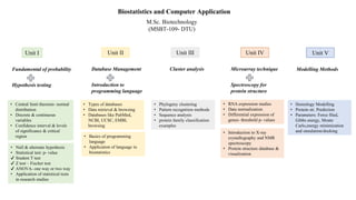
  • 1. Biostatistics and Computer Application M.Sc. Biotechnology (MSBT-109- DTU) Unit I Fundamental of probability Hypothesis testing Unit II Database Management Introduction to programming language Unit III Cluster analysis Unit IV Microarray technique Spectroscopy for protein structure Unit V Modelling Methods • Homology Modelling • Protein str. Prediction • Parameters: Force filed, Gibbs energy, Monte Carlo,energy minimization and simulation/docking • RNA expression studies • Data normalization • Differential expression of genes- threshold p- values • Introduction to X-ray crystallography and NMR spectroscopy • Protein structure database & visualization • Phylogeny clustering • Pattern recognition methods • Sequence analysis • protein family classification examples • Types of databases • Data retrieval & browsing • Databases like PubMed, NCBI, UCSC, EMBL browsing • Central limit theorem- normal distribution • Discrete & continuous variables • Confidence interval & levels of significance & critical region • Basics of programming language • Application of language in biostatistics • Null & alternate hypothesis • Statistical test: p- value ✔ Student T test ✔ Z test – Fischer test ✔ ANOVA- one way or two way • Application of statistical tests in research studies
  • 3. What is Statistics Statistics is the area of applied math that deals with the collection, organization, analysis, interpretation, and presentation of data. Biostatistics is the application of statistical techniques to scientific research in health-related fields, including medicine, biology, and public health. Two main branches of Statistics: • Descriptive Statistics • Inferential Statistics Descriptive statistics focus on describing the visible characteristics of a dataset. A data set is a collection of responses or observations from a sample or entire population. They represent all of the procedures that can be used to organise, summarise, display, and categorise data collected for a certain experiment or event. It includes tabulation, graphical presentation, measures of central tendency, etc Inferential statistics focus on making predictions or generalizations about a larger dataset, based on a sample of those data. The inferential statistics include z test, t test, analysis of variance, etc. In short statistics are about summarizing and answering question based on data. A measurement or datum is a single observation. Data (plural) are a collection of scores.
  • 4. Descriptive statistics • Describe the features of populations and/or samples • Organize and present data in a purely factual way • Present final results visually, using tables, charts, or graphs • Draw conclusions based on known data • Use measures like central tendency, distribution, and variance Descriptive Statistics
  • 5. Descriptive Statistics Descriptive Statistics are used to summarize, organize and simplify data
  • 7. Inferential statistics Use samples to make generalizations about larger populations Help us to make estimates and predict future outcomes Present final results in the form of probabilities Draw conclusions that go beyond the available data Use techniques like hypothesis testing, confidence intervals, and regression and correlation analysis Inferential Statistics
  • 8. • The population may be defined as the entire number of observations that constitute a particular group. Samples are generally a relatively small group of observations that have been taken from a defined population. • Parameters are characteristics of populations while statistic are characteristics of samples representing summary measures computed on observed sample values. • Parameters or population values are usually represented by Greek symbols (e.g. μ) and sample statistic are denoted by letters (e.g. x ̄ ) Population and Samples
  • 9. Population and Samples Ques: what’s the mean diastolic blood pressure of the given population? Sampling error: The discrepancy between the sample statistic and the true population parameter it is estimating. To reduce the sampling error: ✔ Sufficiently large sample size ✔ Random selection (unbiased sample collection)
  • 10. ⮚ Problem Solving ⮚ Use in Clinical Trials ⮚ Use in Manufacturing of Pharmaceuticals ⮚ Use in Quality Control of Pharmaceuticals ⮚ Use in Research and Development of Drugs and Technology ⮚ Use in Anatomy and Physiology ⮚ Use in Pharmacology and Medicine ⮚ Use in Community Medicine and Public Health ⮚ Use in Health and Vital statistics ⮚ Use in Biotechnology, Bioinformatics and Computational Biotechnology Applications and Uses of Biostatistics
  • 11. Variables and Constants ✔ A constant is a characteristic that is fixed across conditions. For example: fingerprint, country in which you were born, genotype. ✔ A variable is something that changes across conditions. For example salary, age, marital status, respiratory rate, blood type etc. Data are the values we get when we measure or observe a variable. ✔ How do we measure things? Qualitatively: By putting them into categories Quantitatively: By using numbers
  • 12. A typical characteristics of this variable are that they do not have any units of measurement, and the ordering of the categories is completely arbitrary. Example: Blood group types - Nominal categorical variable This data too do not have any units of measurement as like that of nominal variables but the ordering of the categories is not arbitrary as it was with nominal variables. Example: Scoring of a patients- Ordinal Ordinal data are not real numbers. They cannot be placed on the number line. As ordinal data are not real numbers, it is not appropriate to apply any of the rules of basic arithmetic to sort this data Nominal Variable Continuous Variable With metric variables, proper measurement is possible and therefore these variables produce data that are real numbers, and can be placed on the number line. Metric continuous variables can be properly measured and have units of measurement. Example: Birth weight (g), blood pressure (mmHg)- Metric continuous Continuous metric data usually comes from measuring while discrete metric data, usually comes from counting The data produced are real numbers, and are invariably integer (i.e. whole number). They can be placed on the number line, and have the same interval and ratio properties as continuous metric data. Metric discrete variables can be properly counted and have units of measurement- ‘numbers of things’. Example: Number of deaths, number of pressure sores, number of angina Attacks- discrete variables Discrete Variable Ordinal Variable Variables
  • 13.
  • 14. Identify type of variable: 1. Dosage form - tablet/ capsule / ointment 2. Bioavailability measurements (C ,T ,AUC) 3. Age ( in years). 4. Hypertension -Mild, Moderate and Severe 5. Smoking history (cigarattes per day) 6. Test- pass or fail criteria 7. Weight 8. Male vs female subjects 9. Scores for patient responses to treatment
  • 16. 1. Biostatistics is branch of statistics applied to_______ science whereby collection, classification, summarising, analysis and interpretation of data is done. a. pharmaceutical b. medicinal c. biological d. chemical 2. Descriptive statistics represents all of the procedures that can be used to_______. a. organise, summarise b. display and categorise c. a & b d. none of above 3. The population is_________. a. the entire number of observations that constitutes a particular group. b. the entire number of samples that constitutes a particular group. c. a & b d. None of above 4. Categorical variable can be divided into__________. a. Nominal & continuous b. nominal & discrete c. discrete&continuous d. nominal&ordinal 5. Metric data can be divided into___________. a. Nominal & continuous b. nominal & discrete c. discrete&continuous d. nominal&ordinal 6. The goal of ___________ is to focus on summarizing and explaining a specific set of data. a. inferential statistics b. descriptive statistics c. none of the above d. all of the above 7. Metric variable can be properly_________. a. measured b. counted c. a & b d. none of the above 8. In categorical variables, values are in ________ categories. a. arbitrary & counted b. arbitrary & measured c. arbitrary & ordered d. counted & measured. 9. Bioavailability measurement is a ___________ variable. a. metric continuous b. metric discrete c. categorical continuous d. categorical ordinal. 10. Scores for patient responses to treatment is a ____________ variable. a. metric continuous b. metric discrete c. categorical continuous d. categorical ordinal Fundamental of Biostatistics- Basic concepts and terminologies
  • 17. Gender Eye Color Identify type of variable: Ethnicity Places in a Race Olympics medals Cloth sizes
  • 19. 01 02 04 03 Frequency Distribution Graphical representations Shape of data distribution Central tendency and dispersion Learning objectives
  • 20. Fundamental of Biostatistics- Data Representation and Distribution ▪ Whenever the data is collected for some project, it is usually in the ‘raw’ form and not in a organised way. ▪ Descriptive statistics deals with sorting this raw data by putting it into a table or by presenting it in an appropriate chart or summarising it numerically. ▪ An important consideration in sorting the raw data is the type of variable concerned. The data from some variables are best described with a table, some with a chart, and some with both. However, a numeric summary is more appropriate for some types of variable ▪ Tabulation is the first step before the data is used for analysis or interpretation. ▪ Frequency distribution tables presents data in a relatively compact form, ready to use but certain information may be lost. The data can be reduced to manageable form using frequency tables. It can have one or all the following parameters, depending on the type of data. 1. Frequency tells you how often something happened OR number of times that any particular value come in a data. 2. Relative frequency is the frequency converted into percentage of the total number of observations. 3. Cumulative frequency is the cumulative total of frequencies and is obtained by adding the frequency of observations at each level point to those frequencies of the preceding level(s). 4. Cumulative relative frequency It is cumulative frequency converted into the percentage of the total number of observations.
  • 21. ⮚ Frequency distribution in nominal data Shows that a higher percentage of nurses than of doctors work in rural areas, but that, overall, a greater proportion of staff works in urban areas (67%). ⮚ It makes no sense to calculate cumulative frequency for nominal data, because of the arbitrary category order. Hence, cumulative frequency is not calculated. But can be done for the ordinal data. The Cumulative and relative cumulative frequency distributions for data Frequency tables can show either categorical variables (sometimes called qualitative variables) or quantitative variables (numeric values). Relative frequency table showing the percentage of students in each blood group
  • 22. ⮚ The most useful approach with metric continuous data is to group them first, and then construct a frequency distribution of the grouped data. It requires major components: class, class limits, boundaries and intervals. Also class marks and open ended groups can be used. • Class: (range of data points) ÷ (range of classes) eg 20 ÷ 5 = 4 • Class size: Difference between the lower and upper class-limits. • Class limit: Represent the smallest and largest data values that can belong to each class. • Class interval: Difference between the upper and lower class limit • Classmark : Average of the upper and lower limits of a class.
  • 23. The frequency distribution table for metric discrete data The relative, cumulative and relative cumulative frequency distribution table ⮚ Grouped frequency table: Exclusive Class Interval: the upper limit of one class is the same as the lower limit of the succeeding class. Note that in continuous cases, any observation corresponding to the extreme values of a class is always included in that class where it is the lower limit. For example, if we had a student who has scored 5 marks in the test, his marks would be included in the class interval 5-10 and not 0-5. Inclusive Class interval: the lower limit of a class does not get repeated in the upper limit of the preceding class. When a frequency distribution is analyzed the iinclusive class interval has to be converted to an exclusive class interval. This can be done by subtracting 0.5 from the lower class limit and adding 0.5 to the upper class limit.
  • 24. Practice question Construct a frequency table for the data on marks obtained by 20 students in their math exam. 20,43,74,89,75,60,31,43,37,36,50,38,21,99,93,45,64,92,38,60 Class Freq Relative freq Cumulative freq Relative Cumulative freq 20-40 40-60 60-80 80-100
  • 25. ⮚ Graphical presentation of data with appropriate chart is a good idea for describing data effectively. Appropriate chart depends primarily on the type of data, as well as on what particular features of it we are looking for. ✔ The Graphical Presentation of Data 1. Pie chart is a diagram in which the frequencies of the groups are shown in a circle. Each segment (slice) of a pie chart should be proportional to the frequency of the category it represents. A disadvantage of a pie chart is that it can only represent one variable. It can lose clarity if it is used to represent more than four or five categories Pie chart of percentage blood group of pharmacy students Simple bar chart of blood group of pharmacy students Clustered bar chart of blood group of 95 pharmacy students by sex A stacked bar chart of blood group of 95 pharmacy students by sex 2. Bar chart: Its a chart with frequency on the vertical axis and category on the horizontal axis. The simple bar chart is appropriate if only one variable is to be shown. All the bars should be of the same width, and there should be equal spaces between bars. These spaces emphasise the categorical nature of the data 3. Clustered bar chart: If there are more than one group, we can use the clustered bar chart. There are two ways of presenting a clustered bar chart. As it compare the relative sizes of the groups within each category. 4. Stacked bar charts: The bars are now stacked on top of each other. Stacked bar charts are appropriate if we want to compare the total number of subjects in each group but not so good if we want to compare category sizes between groups. 5. Pictograms are similar to bar charts. They present the same type of information, but the bars are replaced with a proportional number of icons. This type of presentation for descriptive statistics dates back to the beginning of civilization when pictorial images were used to record numbers of people, animals or objects. Population of different districts of Western Maharashtra. Each diagram indicates one lakh
  • 26. 6. Line chart is similar to a bar chart except that thin lines, instead of thicker bars, are used to represent the frequency associated with each level of the discrete variable 7. Point plots are identical to line charts, however, instead of a line, a number of points or dots equivalent to the frequency are stacked vertically for each value of the horizontal axis. Also referred to as dot diagram, point plots are useful for small data sets. Line and Point Plot of assay result of 30 amoxicillin tablets 8. A histogram looks like a bar chart but without any gaps between adjacent bars. This emphasises the continuous nature of the underlying variable. - If the groups in the frequency table are all of the same width, then the bars in the histogram will also be of the same width. - One limitation of the histogram is that it can represent only one variable at a time (like the pie chart), and this can make comparisons between two histograms difficult. histogram of the grouped weight in kg 9. A frequency polygon can be constructed by placing a dot at the midpoint (class mark) for each class interval in the histogram and then these dots are connected by straight lines. - This frequency polygon gives a better conception of the shape of the distribution. The class interval midpoint for a section in a histogram is calculated as follows: Midpoint = (highest + lowest point)/2 - The frequency polygon is then created by listing the midpoints (class marks) on the x axis, frequencies on the y-axis, and drawing lines to connect the midpoints for each interval. A Frequency Polygon of the grouped weight in kg
  • 27. Ogive of the grouped weight of 60 final year students 10. Relative Cumulative Frequency Curve (Ogive) is a graph of the cumulative relative frequency distribution. ⮚ So, to draw Ogive we should convert ordinary frequency distribution into relative cumulative frequency. ⮚ With continuous metric data, there is assumed to be a smooth continuum of values, so we can chart relative cumulative frequency with a correspondingly smooth curve, or ogive. ✔ By using Ogive we can locate any percentile that will divide the series into parts. ▪ Quartiles: There are three different points located on the entire range of variable. By using these quartiles we can calculate semi inter quartile range and inter quartile range (Q1-Q3). - Q1 or lower quartile will have 25% observations falling in its left and 75% observations on its right side. - Q2 is the median, i.e.,50%values lies on either side. - Q3 is the upper quartile, will have 75% observations falling on its left side and 25% observations on its right side. ▪ Deciles: This divides the distribution into 10 equal parts. First decile (10th percentile) will have 10% values to its left and 90% values to its right. 5th decile is the median and contains 50% values on either side. ▪ Quintiles: This divides the distribution into 5 equal parts. So, 20th percentile or 1st quintile will have 20% observations falling to its left and 80% to its right.
  • 29. 12. The stem-and-leaf plot is a visual representation for continuous data and contains features common to both the frequency distribution and dot diagrams. Digits, instead of bars are used to illustrate the spread and shape of the distribution. Each piece of data is divided into "leading" and "trailing" digits. All the leading digits are sorted from lowest to highest and listed to the left of a vertical line. These digits become the stem. The trailing digits are then written in the appropriate location to the right of the vertical line. These become the leaves. 11. Box-whisker plot: This plot that displays a great deal of information about a continuous variable is the box-and-whisker plot. It shows the bulk of the data as a rectangular box in which the upper and lower lines represent the third quartile (75% of observations below Q3) and first quartile (25% of observations below Ql), respectively. The second quartile (50% of the observations below this point) is depicted as a horizontal line through the box. Vertical lines (whiskers) extend from the top and bottom lines of the box to an upper and lower adjacent value. 13. A scatter diagram is an extremely useful presentation for showing the relationship between two continuous variables. The two dimensional plot has both horizontal and vertical axes which cover the ranges of the two variables. Plotted data points represent paired observations for both the x and y variable. These types of plots are valuable for correlation and regression inferential tests. 14. Time series plot: If the data collected are from measurements made at regular intervals of time (minutes, weeks, years, etc.), we can present the data with a time series chart. Usually these charts are used with metric data, but may also be appropriate for ordinal data. Time is always plotted on the horizontal axis, and data values on the vertical axis.
  • 30. 1. The values are fairly evenly spread throughout their possible range. This is a uniform distribution. 2. The values are concentrated towards the bottom of the range, with progressively fewer values towards the top of the range. This is a right or positively skewed distribution. 3. The values are concentrated towards the top of the range, with progressively fewer values towards the bottom of the range. This is a left or negatively skewed distribution. 4. The values are clumped together around one particular value, with progressively fewer values both below and above this value. This is a symmetric or mound-shaped distribution. 5. The values are clumped around two or more particular values. This is a bimodal or multimodal distribution. ✔ There is one particular symmetric bell-shaped distribution, known as the Normal distribution. Many human clinical features are distributed normally The choice of the most appropriate procedures for summarising and analysing data will not only depend on the type of variable but also on the shape of the distribution. Fundamental of Biostatistics- Data Distribution
  • 31. ✔ It is bell shaped curve ✔ It is symmetrical in distribution; variables on either side of mean are equal in number. ✔ Its maximum height is at the mean. ✔ Mean= mode= median , in case of normal distribution coincide. ✔ Skewness of the curve is zero. ✔ It is asymptotic, in that tails never touch baseline. ✔ Total area of curve is one and standard deviation is also one. ✔ It has two curves. Central part is convex and when it comes down, it becomes concave on both sides. Skewness measures asymmetry around the mean. The parameter is best interpreted as relative to the normal distribution (whose skewness equals to zero). The interpretation of the skewness is : ⮚ Skewness > 0 asymmetric tail with more values above the mean ⮚ Skewness < 0 asymmetric tail with more values below the mean Skewed data is required to be treated using non parametric tests while normal curve data is treated using parametric tests. Kurtosis is a property associated with a frequency distribution and refers to the shape of the distribution of values regarding its relative flatness and peaked-ness. Compared with normal distribution, the interpretation of the kurtosis is: ⮚ Kurtosis > 0 peaked relative to Normal distribution ⮚ Kurtosis < 0 flat relative to Normal distribution
  • 32. ⮚ In any research, enormous data is collected and, to describe it meaningfully, one needs to summarise the same. ⮚ The bulkiness of the data can be reduced by organising it into a frequency table or histogram. ⮚ Frequency distribution organises the heap of data into a few meaningful categories. ⮚ Collected data can also be summarised as a single index/value, which represents the entire data. ⮚ These measures may also help in the comparison of data. ✔ Defined as “the statistical measure that identifies a single value as representative of an entire distribution”. ✔ It aims to provide an accurate description of the entire data. ✔ It is the single value that is most typical/representative of the collected data. Mean is generally considered the best measure of central tendency and the most frequently used. However, there are some situations where the other measures of central tendency are preferred. ✔ The mean, median and mode are the three commonly used measures of central tendency. Measure of Central Tendency
  • 33. ❑ Arithmetic mean (or, simply, “mean”) is nothing but the average. It is computed by adding all the values in the data set divided by the number of observations in it. Measure of Central Tendency- Types of Averages ❑ Median is the value which occupies the middle position when all the observations are arranged in an ascending/descending order. It divides the frequency distribution exactly into two halves. 50% of observations in a distribution have scores at or below the median. Hence median is the 50th percentile. Median is also known as ‘positional average’. ❑ Mode is defined as the value that occurs most frequently in the data. Some data sets do not have a mode because each value occurs only once. On the other hand, some data sets can have more than one mode. This happens when the data set has two or more values of equal frequency which is greater than that of any other value. Mode is rarely used as a summary statistic except to describe a bimodal distribution. In a bimodal distribution, the taller peak is called the major mode and the shorter one is the minor mode. Median is preferred to mean when: ✔ There are few extreme scores in the distribution. ✔ Some scores have undetermined values. ✔ There is an open ended distribution. ✔ Data are measured in an ordinal scale. ⮚ Mode is the preferred measure when data are measured in a nominal scale.
  • 34. Measuring dispersion or variations associated with Central Tendency 1. The range is the distance from the smallest value to the largest. Not affected by skewness, but is sensitive to the addition or removal of an outlier value. Range = Lowest value to Highest value. 2. The interquartile range describes the middle 50% of values when ordered from lowest to highest. To find the interquartile range (IQR), ​first find the median (middle value) of the lower and upper half of the data. These values are quartile 1 (Q1) and quartile 3 (Q3). The IQR is the difference between Q3 and Q1. It is not affected either by outliers or skewness, but it does not use all of the information in the data set since it ignores the bottom and top quarter of values. 3. Standard Deviation is a measure which shows how much variation (such as spread, dispersion, spread,) from the mean exists. It indicates a “typical” deviation from the mean. The most widely used measure of dispersion, is based on all values. It is the square root, of the, mean of the squared deviations, from arithmetic mean. In statistics, Variance and standard deviation are related with each other since the square root of variance is considered the standard deviation for the given data set. 4. The mean deviation is defined as a statistical measure that is used to calculate the average deviation from the mean value of the given data set. It uses absolute values instead of squares to circumvent the issue of negative differences between the data points and their means.
  • 35. Population Parameters versus Sample Statistics Biostatistics is to analyze samples in order to make inferences about the population from which the samples were drawn
  • 36. s2 = 472.10/9 = 52.46 s = √52.46 = 7.24
  • 37. Which statistics should be used to describe the distribution below? a. Mean and IQR b. Mean and Standard Deviation c. Median and IQR d. Median and Standard Deviation Q: Salary (in K) of students after PG 35, 50,50,50,56,60,60,75,250 Mean= ~76.2 and SD = ~ 62.3 Median=56 and IQR=17.5 Questions
  • 39. Probability and its fundamental concepts related to biostatistics ⮚ The probability is the likelihood of occurrence of a particular event or chance of occurrence for an event. ⮚ Experiment refers to describe an act which can be repeated under some given conditions. Those experiments whose results depends on chance are called random experiment. Outcomes of an any experiment are called EVENTS. ⮚ Mutually exclusive events: (Incompatible) When two events cannot happen simultaneously in a single trail. Basically, occurrence of any one event precludes the occurrence of another events. (A AND B) = P(AՈB) (A OR B) = P(AUB)
  • 40. Playing with cards How many cards we have in a Deck ?
  • 41. 1. A card is drawn from a well shuffled pack of 52 cards. Find the probability of: (i) ‘2’ of spades (ii) a jack (iii) a king of red colour (iv) a card of diamond (v) a king or a queen (vi) a non-face card (vii) a black face card (viii) a black card (ix) a non-ace (x) non-face card of black colour (xi) neither a spade nor a jack (xii) neither a heart nor a red king 2. A card is drawn at random from a well-shuffled pack of cards numbered 1 to 20. Find the probability of (i) getting a number less than 7 (ii) getting a number divisible by 3. 3. A card is drawn at random from a pack of 52 playing cards. Find the probability that the card drawn is (i) a king (ii) neither a queen nor a jack.
  • 42. ⮚ Independent events: Two or more events are said to be independent, when the outcome of one event is not affected by other outcomes, as they do not effect other. ⮚ Eg. If a coin is tossed twice, the result of second throw is not affected by the result of the first throw. ✔ Single-event: we consider, probability of happening or not happening of single events. It deals with elementary events. ✔ Compound-event: we consider, the joint occurrence of two or more events. It deals with composite events. ✔ Exhaustive-event: Those events whose totality includes all possible outcomes of RANDOM experiment or sample space. ✔ Complementary-event: Let A & B are two events and both of them are mutually exclusive and exhaustive events. Then A is complementary event of B (& VICE-VERSA). ⮚ Dependent events: In these events occurrence or non- occurrence of one event in any one trial affects the probability of other events in other trails. ⮚ Equally likely event are said to be equally likely when one does not occur more often than the others.
  • 43. (A AND B) = P(AՈB) (A OR B) = P(AUB)
  • 44. CLASS-V 30 Aug 2023 None of the students attended the class
  • 46. Experiment, Outcome, and Sample Space An experiment is a process that, when performed, results in one and only one of many observations. These observations are called the outcomes of the experiment. The collection of all outcomes for an experiment is called a sample space. Examples of Experiments, Outcomes, and Sample Spaces Tree diagram, each outcome is represented by a branch of the tree. • help us understand probability concepts by presenting them visually ⮚ tree diagram for the experiment of tossing a coin once Sample space = {H, T}, where H = Head and T = Tail ⮚ Suppose we randomly select two workers from a company and observe whether the worker selected each time is a man or a woman. Sample space = {MM, MW, WM, WW} Tree diagram for one toss of a coin.
  • 47. Simple and Compound Events An event is a collection of one or more of the outcomes of an experiment. A simple event is also called an elementary event, and a compound event is also called a composite event. Simple Event An event that includes one and only one of the (final) outcomes for an experiment is called a simple event and is usually denoted by Ei. Reconsider previous example: on selecting two workers from a company and observing whether the worker selected each time is a man or a woman. Each of the final four outcomes (MM, MW, WM, and WW) for this experiment is a simple event. These four events can be denoted by E1, E2, E3, and E4, respectively. Thus, E1 = {MM}, E2 = {MW}, E3 = {WM}, and E4 = {WW} Compound Event A compound event is a collection of more than one outcome for an experiment. Reconsider the same example on selecting two workers from a company and observing whether the worker selected each time is a man or a woman. Let A be the event that at most one man is selected. Is event A a simple or a compound event? Here at most one man means one or no man is selected. Thus, event A will occur if either no man or one man is selected. Hence, the event A is given by A = at most one man is selected = {MW, WM, WW} Because event A contains more than one outcome, it is a compound event.
  • 48. Q: In a group of college students, some like ice tea and others do not. There is no student in this group who is indifferent or has no opinion. Two students are randomly selected from this group. (a) How many outcomes are possible? List all the possible outcomes. (b) Consider the following events. List all the outcomes included in each of these events. Mention whether each of these events is a simple or a compound event. (i) Both students like ice tea. (ii) At most one student likes ice tea. (iii) At least one student likes ice tea. (iv) Neither student likes ice tea. Let L denote the event that a student likes ice tea and N denote the event that a student does not like ice tea. (a) This experiment has four outcomes, LL = Both students like ice tea L N = The first student likes ice tea but the second student does not NL = The first student does not like ice tea but the second student does NN = Both students do not like ice tea (b) (i) The event both students like ice tea will occur if LL happens. Thus, Both students like ice tea = {L L} Since this event includes only one of the four outcomes, it is a simple event. (ii) The event at most one student likes ice tea will occur if one or none of the two students likes ice tea. At most one student likes ice tea = {L N, NL, N N} Since this event includes three outcomes, it is a compound event. (iii) The event at least one student likes ice tea will occur if one or two of the two students like ice tea. Thus, At least one student likes ice tea = {LN, NL, LL} Since this event includes three outcomes, it is a compound event. (iv) The event neither student likes ice tea will occur if neither of the two students likes ice tea, which will include the event NN. Thus, Neither student likes ice tea = {NN} Since this event includes one outcome, it is a simple event.
  • 49. Probability is a numerical measure of the likelihood that a specific event will occur. The probability that a simple event Ei will occur is denoted by P(Ei), and the probability that a compound event A will occur is denoted by P(A). Two Properties of Probability 1. The probability of an event always lies in the range 0 to 1. Whether it is a simple or a compound event, the probability of an event is never less than 0 or greater than 1. 0 ≤ P(Ei) ≤ 1 0 ≤ P(A) ≤ 1 2. The sum of the probabilities of all simple events (or final outcomes) for an experiment, denoted by ΣP(Ei), is always 1. For an experiment with outcomes E1, E2, E3, .a . . , ΣP(Ei) = P(E1) + P(E2) + P(E3) + . . . = 1.0 Classical Probability: Equally Likely Outcomes Two or more outcomes that have the same probability of occurrence are said to be equally likely outcomes.
  • 50. Marginal probability is the probability of a single event without consideration of any other event. Example: 15 employees in this group possess two characteristics: “male” and “in favor of paying high salaries to CEOs.” Suppose one employee is selected at random from these 100 employees. If only one characteristic is considered at a time, the employee selected can be a male, a female, in favor, or against. The probability of each of these four characteristics or events is called marginal probability. The four marginal probabilities are calculated as follows: P(male) = Number of males/ Total number of employees = 60/100 = .60 As we can observe, the probability that a male will be selected is obtained by dividing the total of the row labeled “Male” (60) by the grand total (100). Similarly, P(female) = 40/100 = .40 P(in favor) = 19/100 = .19 P(against) = 81/100 = .81
  • 51. Now suppose that one employee is selected at random from these 100 employees. Furthermore, assume it is known that this (selected) employee is a male. In other words, the event that the employee selected is a male has already occurred. Given that this selected employee is a male, he can be in favor or against. What is the probability that the employee selected is in favor of paying high salaries to CEOs? Conditional probability is the probability that an event will occur given that another event has already occurred. If A and B are two events, then the conditional probability of A given B is written as P(A ∣ B) and read as “the probability of A given that B has already occurred.”
  • 52. Mutually Exclusive Events : Events that cannot occur together are said to be mutually exclusive events. Consider the following events for one roll of a die: A = an even number is observed = {2, 4, 6} B = an odd number is observed = {1, 3, 5} C = a number less than 5 is observed = {1, 2, 3, 4} Are events A and B mutually exclusive? Are events A and C mutually exclusive? Independent Events Two events are said to be independent if the occurrence of one event does not affect the probability of the occurrence of the other event. In other words, A and B are independent events if either P(A ∣ B) = P(A) or P(B ∣ A) = P(B) Complementary Events: The complement of event A, denoted by A and read as “A bar” or “A complement,” is the event that includes all the outcomes for an experiment that are not in A. Events A and A are complements of each other. Because two complementary events, taken together, include all the outcomes for an experiment and because the sum of the probabilities of all outcomes is 1, it is obvious that P(A) + P(A) = 1.0 Question: Of the 500 adults, 325 drink coffee with sugar. Suppose one adult is randomly selected from these 500 adults, and let A be the event that this adult drinks coffee with sugar. What is the complement of event A? What are the probabilities of the two events? Mutually exclusive events A and B. Mutually nonexclusive events A and C.
  • 53. Theorem of probability Joint Probability The probability of the intersection of two events is called their joint probability. It is written as P(A and B)
  • 54.
  • 55. Union of Events : Let A and B be two events defined in a sample space. The union of events A and B is the collection of all outcomes that belong either to A or to B or to both A and B and is denoted by (A or B); (A ∪ B)
  • 56.
  • 57. Counting Rule: to Find Total Outcomes If an experiment consists of three steps, and if the first step can result in m outcomes, the second step in n outcomes, and the third step in k outcomes, then Total outcomes for the experiment = m · n · k The symbol ! (read as factorial) is used to denote factorials. The value of the factorial of a numberis obtained by multiplying all the integers from that number to 1. For example, 7! is read as “seven factorial” and is evaluated by multiplying all the integers from 7 to 1. Example: Evaluate 7!. Solution To evaluate 7!, we multiply all the integers from 7 to 1. 7!= 7 ⋅ 6 ⋅ 5 ⋅ 4 ⋅ 3 ⋅ 2 ⋅ 1 = 5040 Thus, the value of 7! is 5040. Example: Consider three tosses of a coin. How many total outcomes this experiment has? Solution This experiment of tossing a coin three times. Each step has two outcomes: a head and a tail. Thus, Total outcomes for three tosses of a coin = 2 × 2 × 2 = 8 The eight outcomes for this experiment are HHH, HHT, HTH, HTT, THH, THT, TTH, and TTT. Counting Rule, Factorials
  • 58. Discrete Random Variables and Their Probability Distributions Random Variable: A random variable is a variable whose value is determined by the outcome of a random experiment. Discrete Random Variable A random variable that assumes countable values is called a discrete random variable. examples of discrete random variables • The number of houses in a certain block • The number of customers who visit a bank during any given hour • The number of complaints received at the office of an airline on a given day Continuous Random Variable A random variable that can assume any value contained in one or more intervals is called a continuous random variable. Examples of continuous random variables • The length of a room • The time taken to commute from home to work • The weight of a letter • The price of a house
  • 59. Probability Distribution of a Discrete Random Variable: ⮚ Binomial Probability Distribution ⮚ Poisson Probability Distribution ⮚ Hypergeometric Probability Distribution The Binomial Probability Distribution ✔ most widely used discrete probability distributions. ✔ the random variable x must be a discrete dichotomous random variable. ✔ Each repetition of a binomial experiment is called a trial or a Bernoulli trial. ✔ For example, if an experiment is defined as one toss of a coin and this experiment is repeated 10 times, then each repetition (toss) is called a trial. Consequently, there are 10 total trials for this experiment. An experiment that satisfies the following four conditions is called a binomial experiment. 1. There are n identical trials. In other words, the given experiment is repeated n times, where n is a positive integer. All of these repetitions are performed under identical conditions. 2. Each trial has two and only two outcomes. These outcomes are usually called a success and a failure, respectively. In case there are more than two outcomes for an experiment, we can combine outcomes into two events and then apply binomial probability distribution. 3. The probability of success is denoted by p and that of failure by q, and p + q = 1. The probabilities p and q remain constant for each trial. 4. The trials are independent. In other words, the outcome of one trial does not affect the outcome of another trial. Note: Success does not mean favorable or desirable outcome and a failure does not refer to an unfavorable or undesirable outcome. The outcome to which the question refers is usually called a success; the outcome to which it does not refer is called a failure.
  • 60. n = total number of trials = number of students selected = 3 x = number of successes = number of students in three who use Instagram = 2 p = probability of success = probability that a student uses Instagram = .75 n − x = number of failures = number of students not using Instagram = 3 − 2 = 1 q = probability of failure = probability that a student does not use Instagram = 1 − .75 = .25 The probability of two successes is denoted by P(x = 2) or simply by P(2). Substituting all of the values in the binomial formula Example: Seventy five percent of students at a college with a large student population use the social media site Instagram. Three students are randomly selected from this college. What is the probability that exactly two of these three students use Instagram?
  • 61. Mean and Standard Deviation of the Binomial Distribution U.S. Adults with No Religious Affiliation Example: According to a Pew Research Center survey released on May 12, 2015, 22.8% of U.S. adults do not have a religious affiliation. Assume that this result is true for the current population of U.S. adults. A sample of 50 U.S. adults is randomly selected. Let x be the number of adults in this sample who do not have a religious affiliation. Find the mean and standard deviation of the probability distribution of x. Sol: This is a binomial experiment with a total of 50 trials. Each trial has two outcomes: (1) the selected adult does not have a religious affiliation, (2) the selected adult has a religious affiliation or does not want to answer the question. The probabilities p and q for these two outcomes are .228 and .772, respectively. n = 50, p = .228 and q = .772 mean and standard deviation of the binomial distribution: μ = np = 50(.228) = 11.4 σ = √npq = √(50) (.228) (.772) = 2.9666 The value of the mean is what we expect to obtain, on average, per repetition of the experiment. In this example, if we select many samples of 50 U.S. adults each, we expect that each sample will contain an average of 11.4 adults, with a standard deviation of 2.9666, who will not have a religious affiliation.
  • 62. The Hypergeometric Probability Distribution If the trials are not independent, we cannot apply the binomial probability distribution to find the probability of x successes in n trials. In such cases we replace the binomial probability distribution by the hypergeometric probability distribution Defective Auto Parts in a Shipment Example: Brown Manufacturing makes auto parts that are sold to auto dealers. Last week the company shipped 25 auto parts to a dealer. Later, it found out that 5 of those parts were defective. By the time the company manager contacted the dealer, 4 auto parts from that shipment had already been sold. What is the probability that 3 of those 4 parts were good parts and 1 was defective?
  • 63. Solution Let a good part be called a success and a defective part be called a failure. From the given information, N = total number of elements (auto parts) in the population = 25 r = number of successes (good parts) in the population = 20 N − r = number of failures (defective parts) in the population = 5 n = number of trials (sample size) = 4 x = number of successes in four trials = 3 n − x = number of failures in four trials = 1 Using the hypergeometric formula, we calculate the required probability as follows: Thus, the probability that 3 of the 4 parts sold are good and 1 is defective is .4506.
  • 64. The Poisson Probability Distribution: If the average number of occurrences for a given interval is known, then by using the Poisson probability distribution, we can compute the probability of a certain number of occurrences, x, in that interval. Conditions to Apply the Poisson Probability Distribution The following three conditions must be satisfi ed to apply the Poisson probability distribution. 1. x is a discrete random variable. 2. The occurrences are random. 3. The occurrences are independent. The following examples also qualify for the application of the Poisson probability distribution. 1. The number of accidents that occur on a given highway during a 1-week period 2. The number of customers entering a grocery store during a 1-hour interval 3. The number of television sets sold at a department store during a given week Mean and Standard Deviation of the Poisson Probability Distribution For the Poisson probability distribution, the mean and variance both are equal to λ, and the standard deviation is equal to √λ. That is, for the Poisson probability distribution, μ = λ, σ2 = λ, and σ = √λ
  • 65. Washing Machine Breakdowns A washing machine in a laundromat breaks down an average of three times per month. Using the Poisson probability distribution formula, find the probability that during the next month this machine will have (a) exactly two breakdowns (b) at most one breakdown
  • 66.
  • 67. Continuous Random Variables and the Normal Distribution Total area under a normal curve A normal curve is symmetric about the mean Areas of the normal curve beyond μ ± 3σ. The standard normal distribution is a special case of the normal distribution. For the standard normal distribution, the value of the mean is equal to zero and the value of the standard deviation is equal to 1. Equation of the normal distribution is z Values or z Scores The units marked on the horizontal axis of the standard normal curve are denoted by z and are called the z values or z scores. A specific value of z gives the distance between the mean and the point represented by z in terms of the standard deviation. For example, a point with a value of z = 2 is two standard deviations to the right of the mean. Similarly, a point with a value of z = −2 is two standard deviations to the left of the mean.