Downloaded 13 times
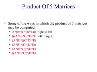
![Iterative Solution Example
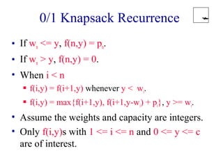
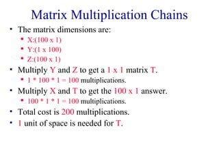
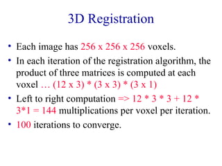
• n = 5, c = 8, w = [4,3,5,6,2], p = [9,7,10,9,3]
f[i][y] 0 1 2 3 4 5 6 7 8
y
5
4
3
2
1
i](https://image.slidesharecdn.com/lec38-140928020032-phpapp01/85/Lec38-4-320.jpg)
![Compute f[5][*]
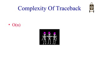
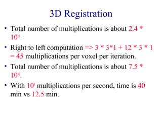
• n = 5, c = 8, w = [4,3,5,6,2], p = [9,7,10,9,3]
f[i][y] 0 1 2 3 4 5 6 7 8
y
5
4
3
2
1
i
0 0 3 3 3 3 3 3 3](https://image.slidesharecdn.com/lec38-140928020032-phpapp01/85/Lec38-5-320.jpg)
![Compute f[4][*]
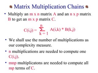
• n = 5, c = 8, w = [4,3,5,6,2], p = [9,8,10,9,3]
f[i][y] 0 1 2 3 4 5 6 7 8
y
5
4
3
2
1
i
0 0 3 3 3 3 3 3 3
0 0 3 3 3 3 9 9 12
f(i,y) = max{f(i+1,y), f(i+1,y-wi) + pi}, y >= wi](https://image.slidesharecdn.com/lec38-140928020032-phpapp01/85/Lec38-6-320.jpg)
![Compute f[3][*]
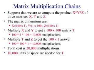
• n = 5, c = 8, w = [4,3,5,6,2], p = [9,8,10,9,3]
f[i][y] 0 1 2 3 4 5 6 7 8
y
5
4
3
2
1
i
0 0 3 3 3 3 3 3 3
0 0 3 3 3 3 9 9 12
0 0 3 3 3 10 10 13 13
f(i,y) = max{f(i+1,y), f(i+1,y-wi) + pi}, y >= wi](https://image.slidesharecdn.com/lec38-140928020032-phpapp01/85/Lec38-7-320.jpg)
![Compute f[2][*]
• n = 5, c = 8, w = [4,3,5,6,2], p = [9,8,10,9,3]
f[i][y] 0 1 2 3 4 5 6 7 8
y
5
4
3
2
1
i
0 0 3 3 3 3 3 3 3
0 0 3 3 3 3 9 9 12
0 0 3 3 3 10 10 13 13
0 0 3 8 8 11 11 13 18
f(i,y) = max{f(i+1,y), f(i+1,y-wi) + pi}, y >= wi](https://image.slidesharecdn.com/lec38-140928020032-phpapp01/85/Lec38-8-320.jpg)
![Compute f[1][c]
• n = 5, c = 8, w = [4,3,5,6,2], p = [9,8,10,9,3]
f[i][y] 0 1 2 3 4 5 6 7 8
y
5
4
3
2
1
i
0 0 3 3 3 3 3 3 3
0 0 3 3 3 3 9 9 12
0 0 3 3 3 10 10 13 13
0 0 3 8 8 11 11 13 18
18
f(i,y) = max{f(i+1,y), f(i+1,y-wi) + pi}, y >= wi](https://image.slidesharecdn.com/lec38-140928020032-phpapp01/85/Lec38-9-320.jpg)
![Traceback
• n = 5, c = 8, w = [4,3,5,6,2], p = [9,8,10,9,3]
f[i][y] 0 1 2 3 4 5 6 7 8
y
5
4
3
2
1
i
0 0 3 3 3 3 3 3 3
0 0 3 3 3 3 9 9 12
0 0 3 3 3 10 10 13 13
0 0 3 8 8 11 11 13 18
18
f[1][8] = f[2][8] => x1 = 0](https://image.slidesharecdn.com/lec38-140928020032-phpapp01/85/Lec38-10-320.jpg)
![Traceback
• n = 5, c = 8, w = [4,3,5,6,2], p = [9,8,10,9,3]
f[i][y] 0 1 2 3 4 5 6 7 8
y
5
4
3
2
1
i
0 0 3 3 3 3 3 3 3
0 0 3 3 3 3 9 9 12
0 0 3 3 3 10
10 13 13
0 0 3 8 8 11 11 13 18
18
f[2][8] != f[3][8] => x2 = 1](https://image.slidesharecdn.com/lec38-140928020032-phpapp01/85/Lec38-11-320.jpg)
![Traceback
• n = 5, c = 8, w = [4,3,5,6,2], p = [9,8,10,9,3]
f[i][y] 0 1 2 3 4 5 6 7 8
y
5
4
3
2
1
i
0 0 3 3 3 3 3 3 3
0
0 3 3 3 3 9 9 12
0 0 3 3 3 10 10 13 13
0 0 3 8 8 11 11 13 18
18
f[3][5] != f[4][5] => x3 = 1](https://image.slidesharecdn.com/lec38-140928020032-phpapp01/85/Lec38-12-320.jpg)
![Traceback
• n = 5, c = 8, w = [4,3,5,6,2], p = [9,8,10,9,3]
f[i][y] 0 1 2 3 4 5 6 7 8
y
5
4
3
2
1
i
0 3 3 3 3 3 3 3
0
0 0 3 3 3 3 9 9 12
0 0 3 3 3 10 10 13 13
0 0 3 8 8 11 11 13 18
18
f[4][0] = f[5][0] => x4 = 0](https://image.slidesharecdn.com/lec38-140928020032-phpapp01/85/Lec38-13-320.jpg)
![Traceback
• n = 5, c = 8, w = [4,3,5,6,2], p = [9,8,10,9,3]
f[i][y] 0 1 2 3 4 5 6 7 8
y
5
4
3
2
1
i
0 0 3 3 3 3 3 3 3
0 0 3 3 3 3 9 9 12
0 0 3 3 3 10 10 13 13
0 0 3 8 8 11 11 13 18
18
f[5][0] = 0 => x5 = 0](https://image.slidesharecdn.com/lec38-140928020032-phpapp01/85/Lec38-14-320.jpg)

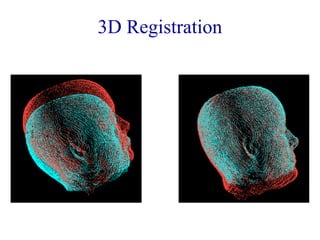

Dynamic programming is an algorithmic technique for solving problems by breaking them down into simpler subproblems. It involves viewing a problem as a sequence of decisions, setting up recurrence relations to calculate optimal solutions, and using these relations to iteratively solve for the overall optimal solution. For problems like the 0/1 knapsack problem, dynamic programming avoids recomputing solutions by storing results in a table. Finding optimal orders for matrix multiplication chains and applying dynamic programming to 3D image registration are examples discussed.