Download to read offline


![Proposed solution
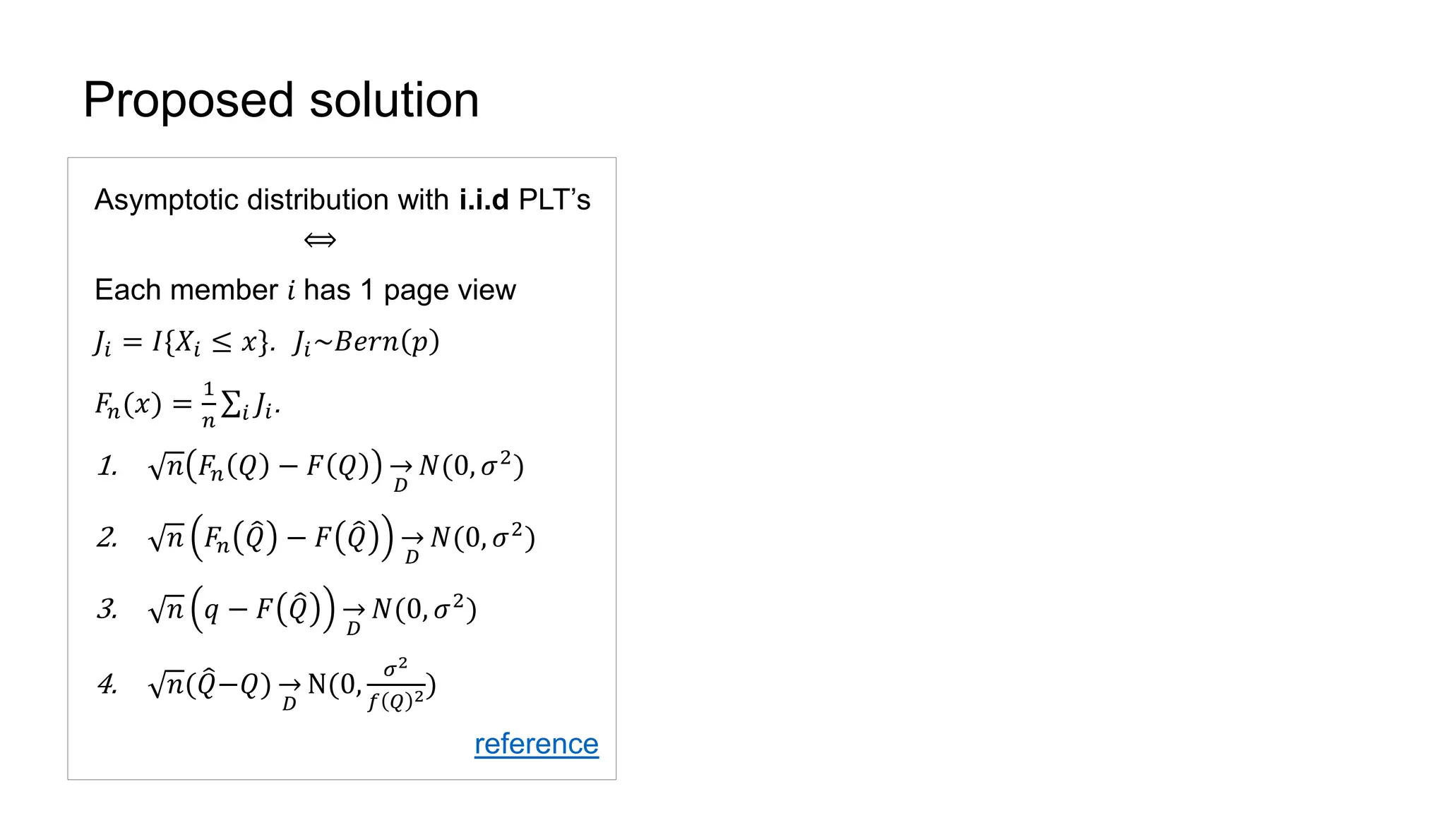
Asymptotic distribution with i.i.d PLT’s
⟺
Each member 𝑖 has 1 page view
𝐽𝑖 = 𝐼{𝑋𝑖 ≤ 𝑥}. 𝐽𝑖~𝐵𝑒𝑟𝑛 𝑝
𝐹𝑛(𝑥) =
1
𝑛 𝑖 𝐽𝑖.
1. 𝑛 𝐹𝑛 𝑄 − 𝐹 𝑄
𝐷
𝑁(0, 𝜎2
)
2. 𝑛 𝐹𝑛 𝑄 − 𝐹 𝑄
𝐷
𝑁(0, 𝜎2
)
3. 𝑛 𝑞 − 𝐹 𝑄
𝐷
𝑁(0, 𝜎2
)
4. 𝑛( 𝑄−𝑄)
𝐷
N(0,
𝜎2
𝑓 𝑄 2)
reference
Asymptotic distribution with non-i.i.d PLT’s
𝐽𝑖 = 𝑗 𝐼 𝑋𝑖,𝑗 ≤ 𝑥 . 𝐽𝑖’s are i.i.d
𝑌𝑛(𝑥) =
1
𝑛 𝑖 𝐽𝑖 and 𝑃𝑛 =
1
𝑛 𝑖 𝑃𝑖. 𝐹𝑛(𝑥) =
𝑌𝑛 𝑥
𝑃 𝑛
0. 𝑛[ 𝑌𝑛 𝑄
𝑃 𝑛
− 𝜇 𝐽
𝜇 𝑃
]
𝐷
𝑁(0, Σ)
1. 𝑛(𝐹𝑛(𝑄) − 𝐹(𝑄))
𝐷
𝑁(0, 𝜎 𝑃,𝐽
2
)
where 𝐹 𝑄 =
𝐹 𝑄 𝜇 𝑃
𝜇 𝑃
=
𝐸[𝐸(𝐽 𝑖|𝑃 𝑖)]
𝜇 𝑃
=
𝜇 𝐽
𝜇 𝑃
2. 𝑛 𝐹𝑛 𝑄 − 𝐹 𝑄
𝐷
𝑁(0, 𝜎 𝑃,𝐽
2
)
3. 𝑛 𝑞 − 𝐹 𝑄
𝐷
𝑁(0, 𝜎 𝑃,𝐽
2
)
4. 𝑛( 𝑄−𝑄)
𝐷
N(0,
𝜎 𝑃,𝐽
2
𝑓 𝑄 2)](https://image.slidesharecdn.com/largescalequantilemetrics-181218182142/75/Large-Scale-Online-Experimentation-with-Quantile-Metrics-15-2048.jpg)
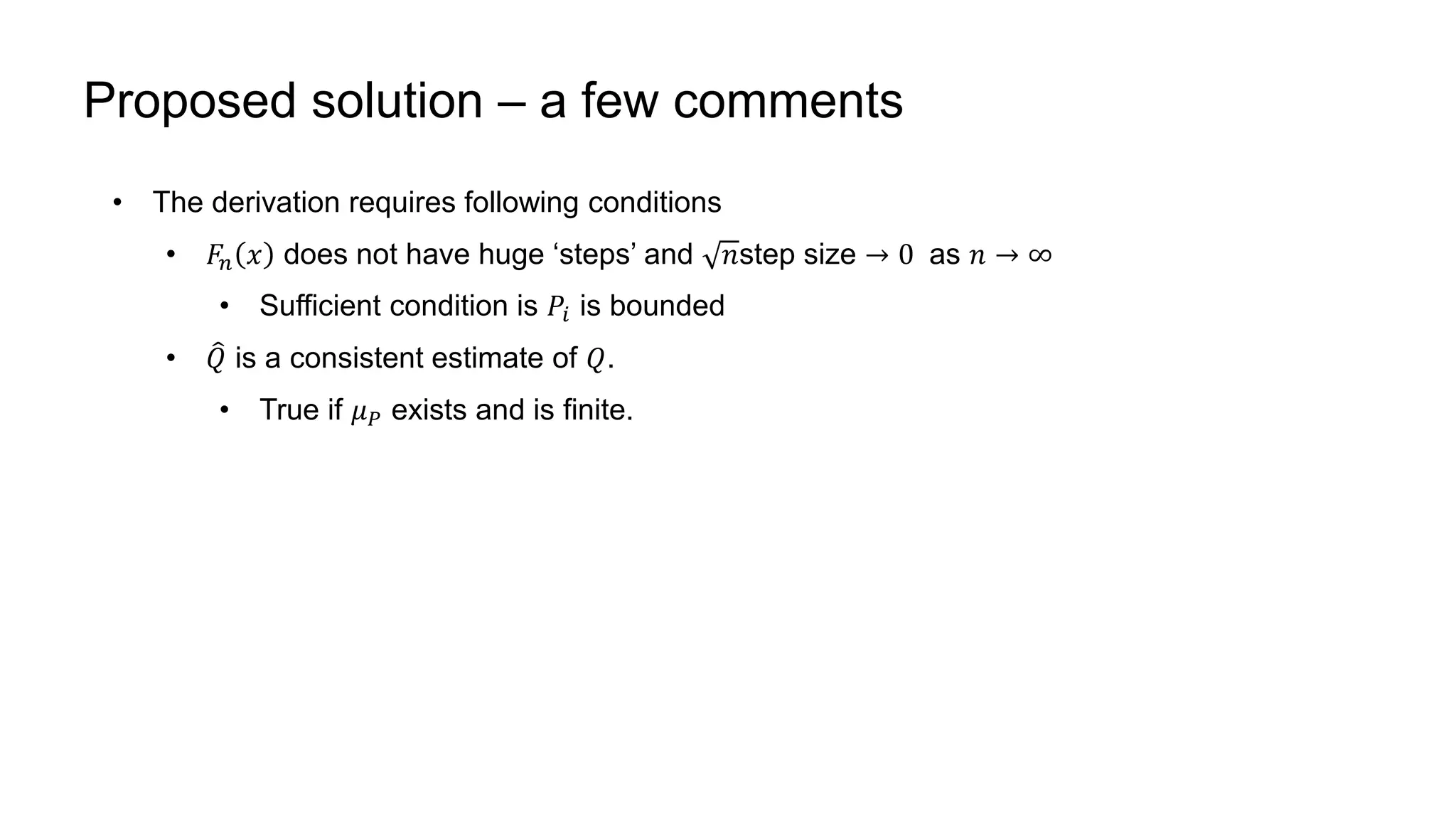
![Proposed solution – a few comments
• 𝑓(𝑄) estimated by average density in a window ( 𝑄 − 𝛿, 𝑄 + 𝛿]
• 𝛿 set to 50ms for initial estimate
• Then set to 2 × 𝑠𝑡𝑑𝑑𝑒𝑣, turns out to be very effective in reducing estimation error](https://image.slidesharecdn.com/largescalequantilemetrics-181218182142/75/Large-Scale-Online-Experimentation-with-Quantile-Metrics-17-2048.jpg)

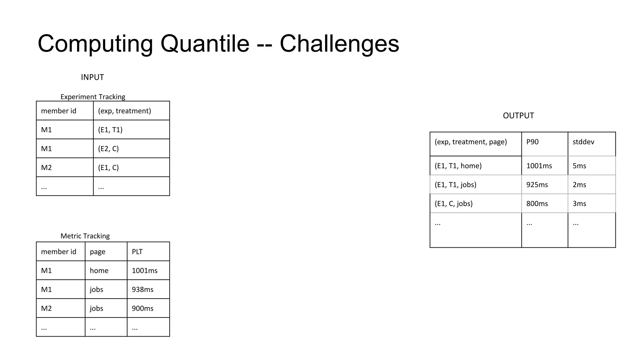
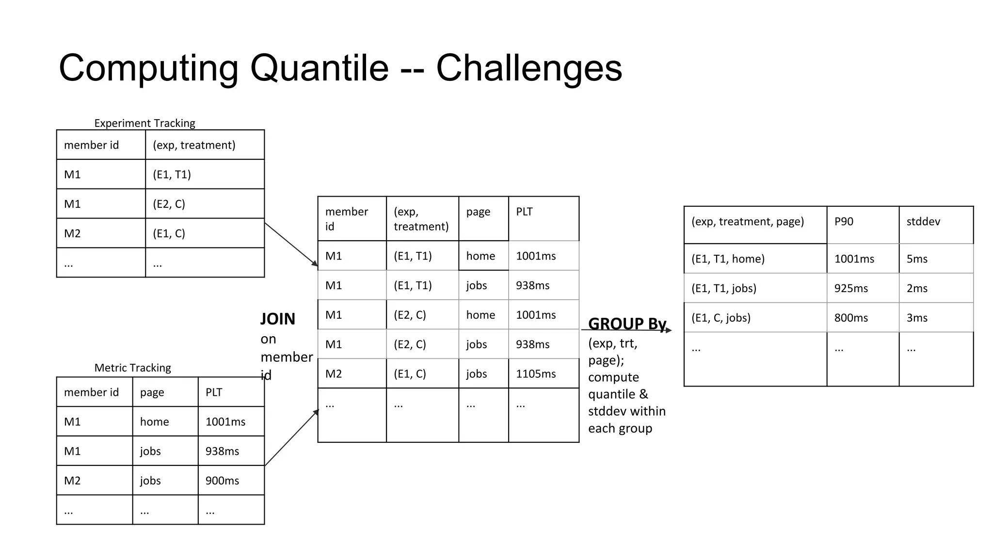
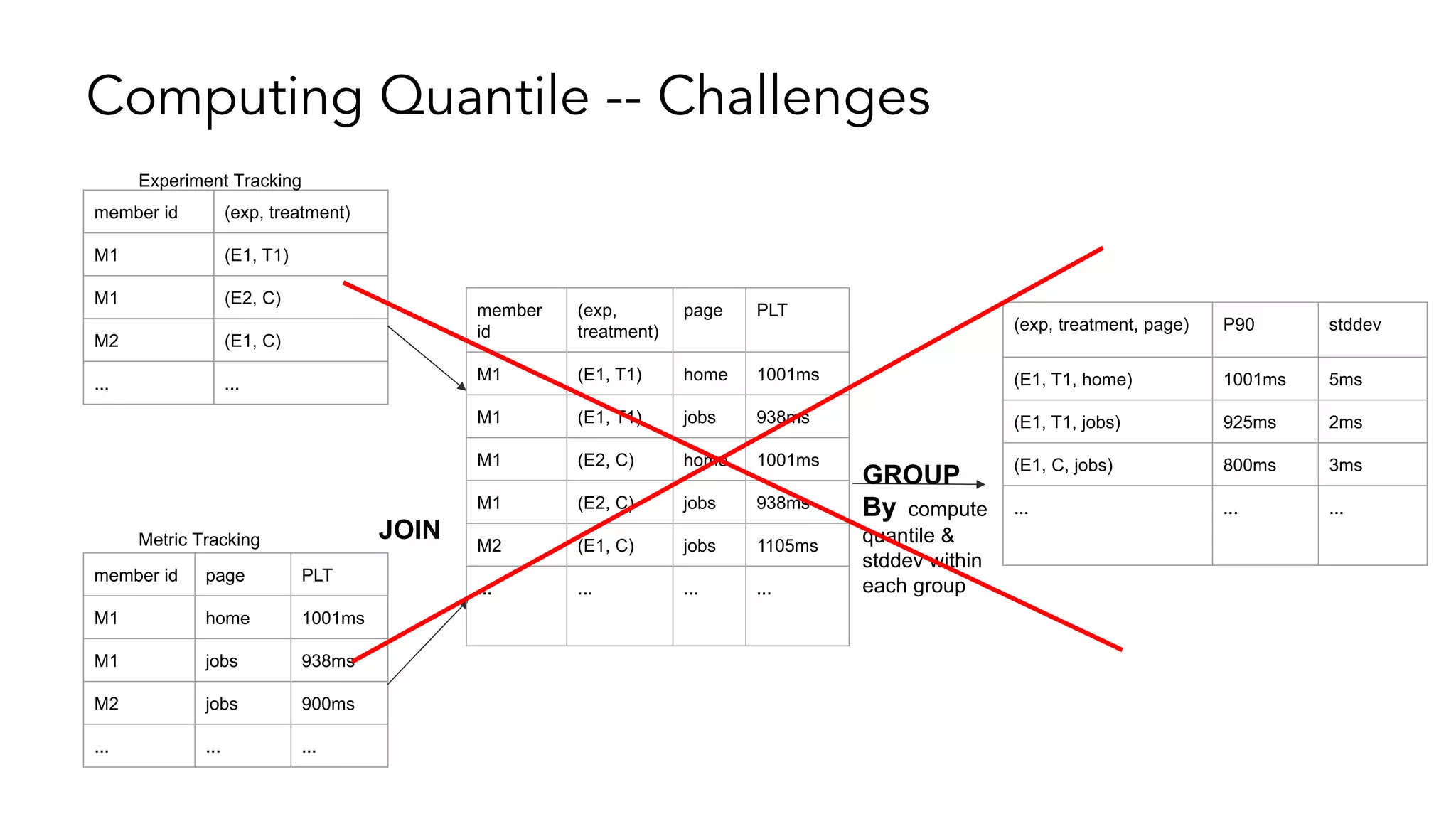
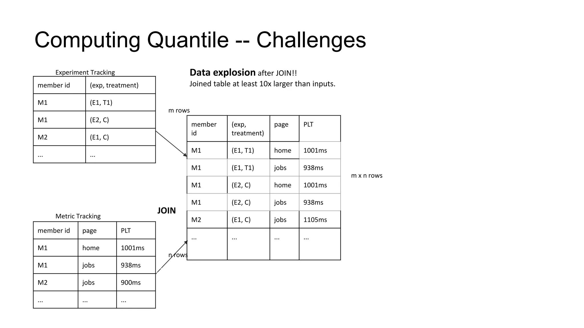
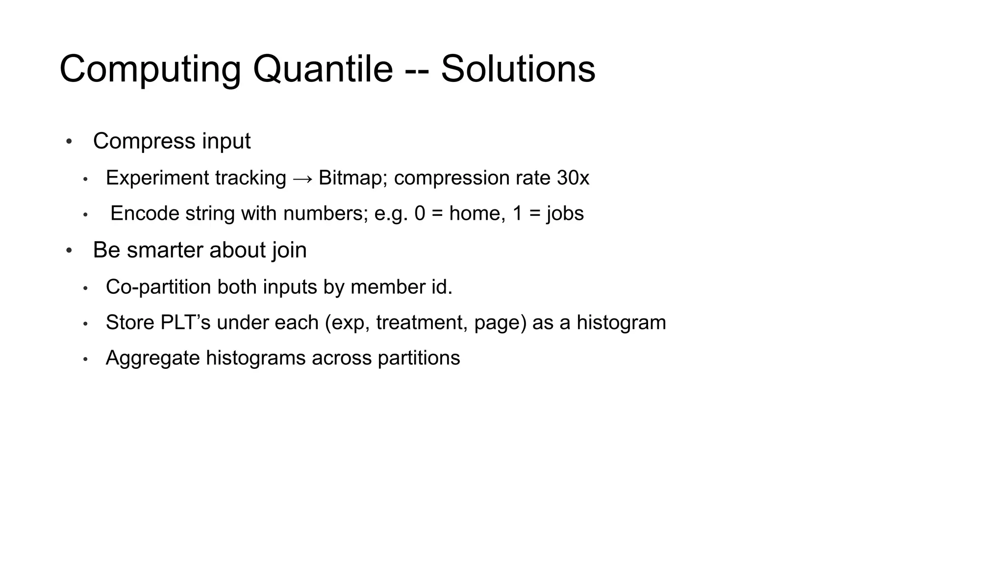
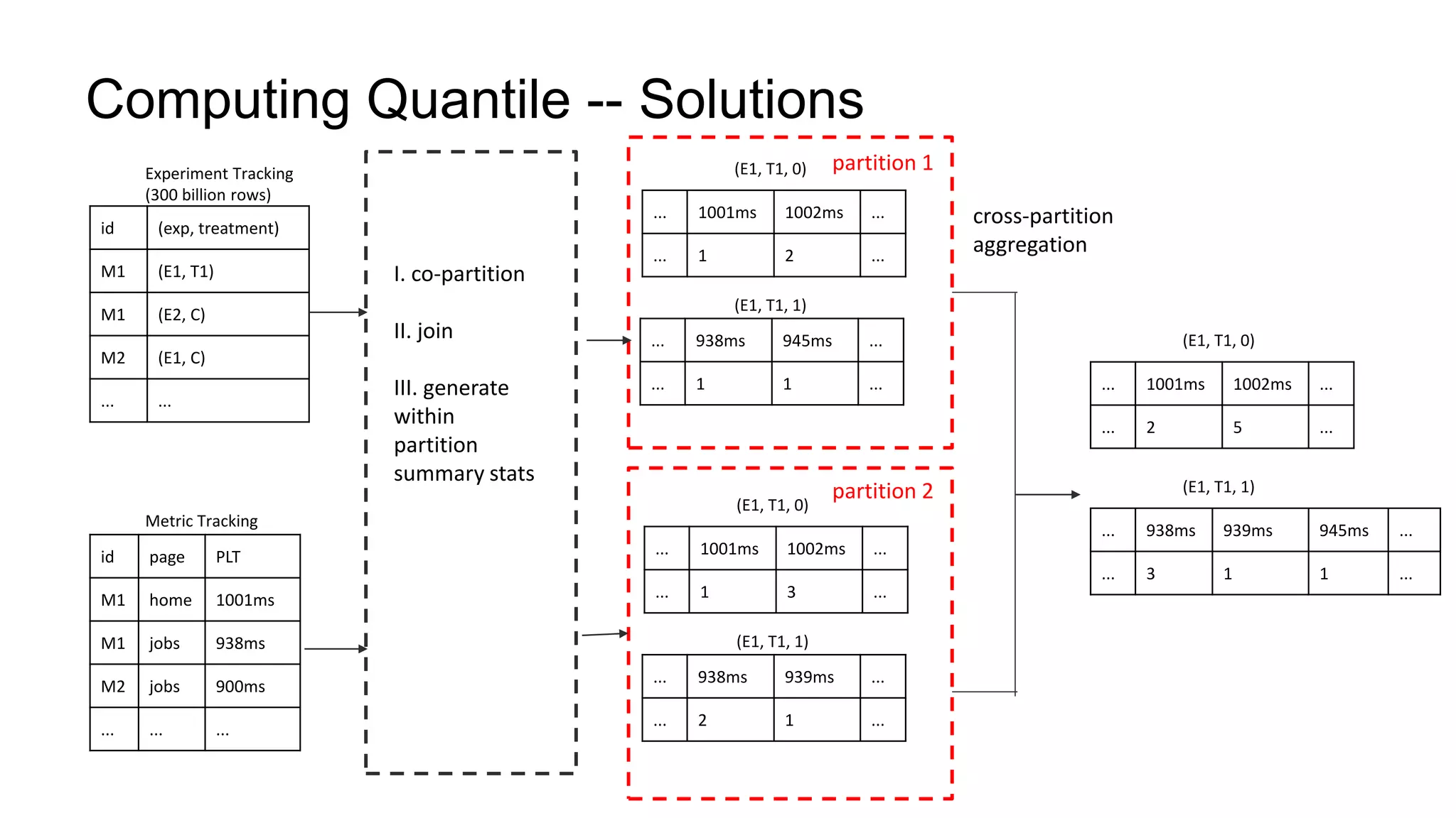
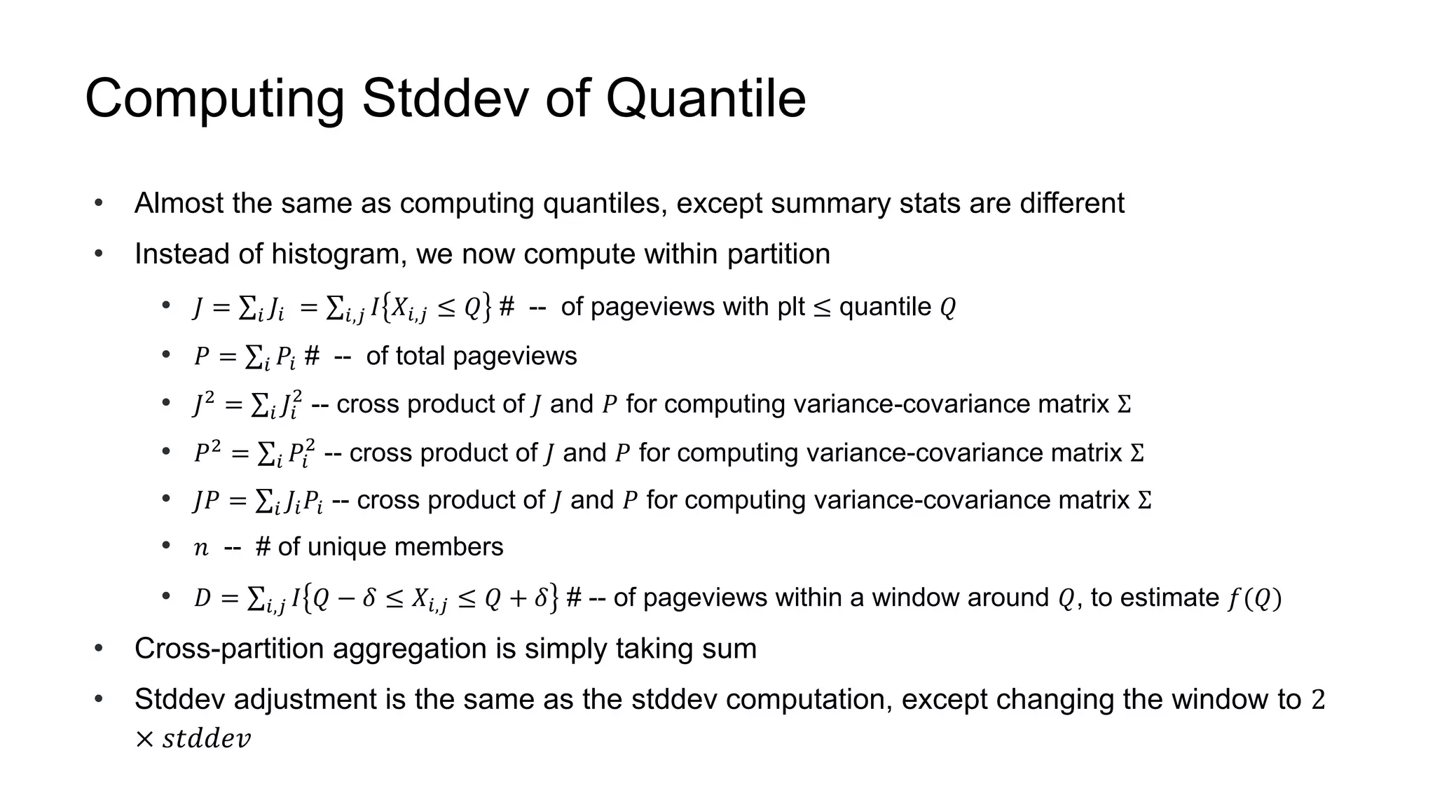

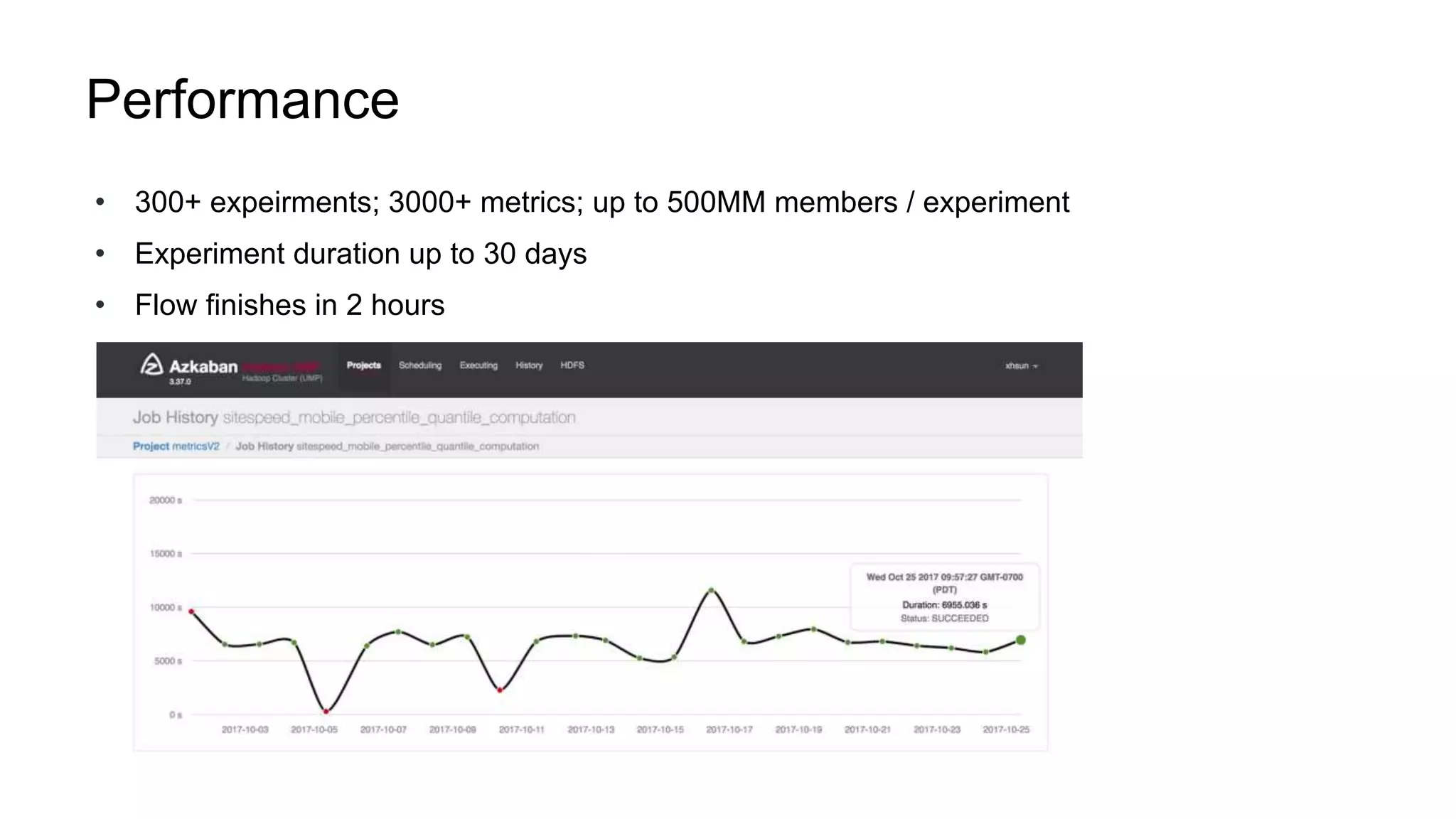
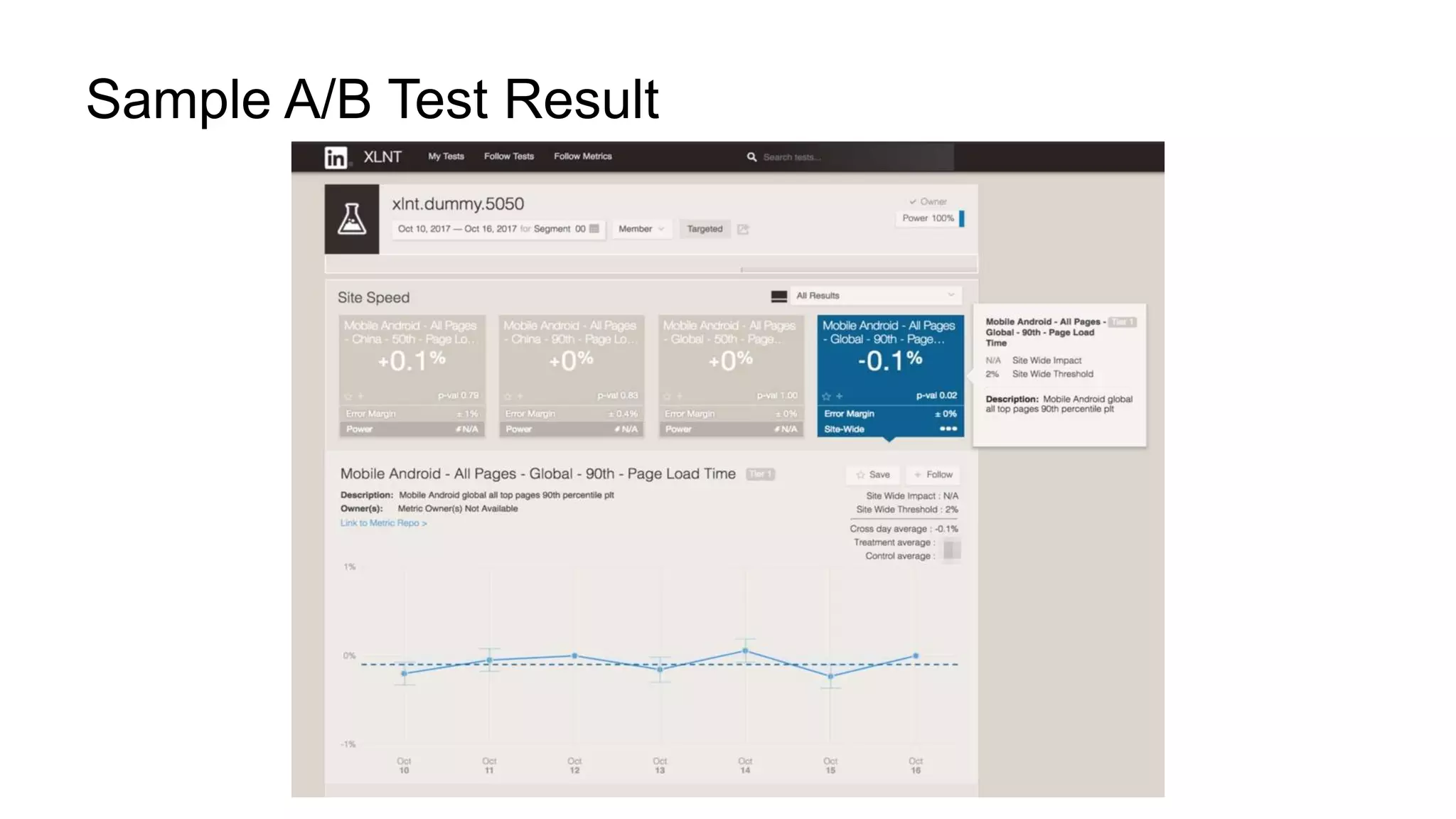

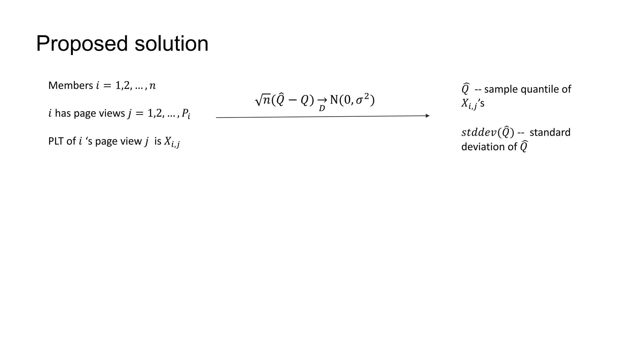
The document describes a methodology for conducting large-scale online experiments using quantile metrics. It outlines three key challenges: 1) ensuring experiments are statistically valid and scalable given hundreds of concurrent tests involving billions of data points, 2) existing solutions are either statistically valid or scalable but not both, and 3) protecting users from slow experiences by detecting degradation in page load time quantiles like P90. The proposed solution provides statistically valid quantile estimates while being 500x faster than traditional bootstrapping through an asymptotic distribution approximation, compressed data representations, and optimized pipeline design that involves co-partitioning and aggregating histogram summaries across partitions. Results demonstrated the ability to analyze over 300 experiments, 3000 metrics, and up to 500 million members