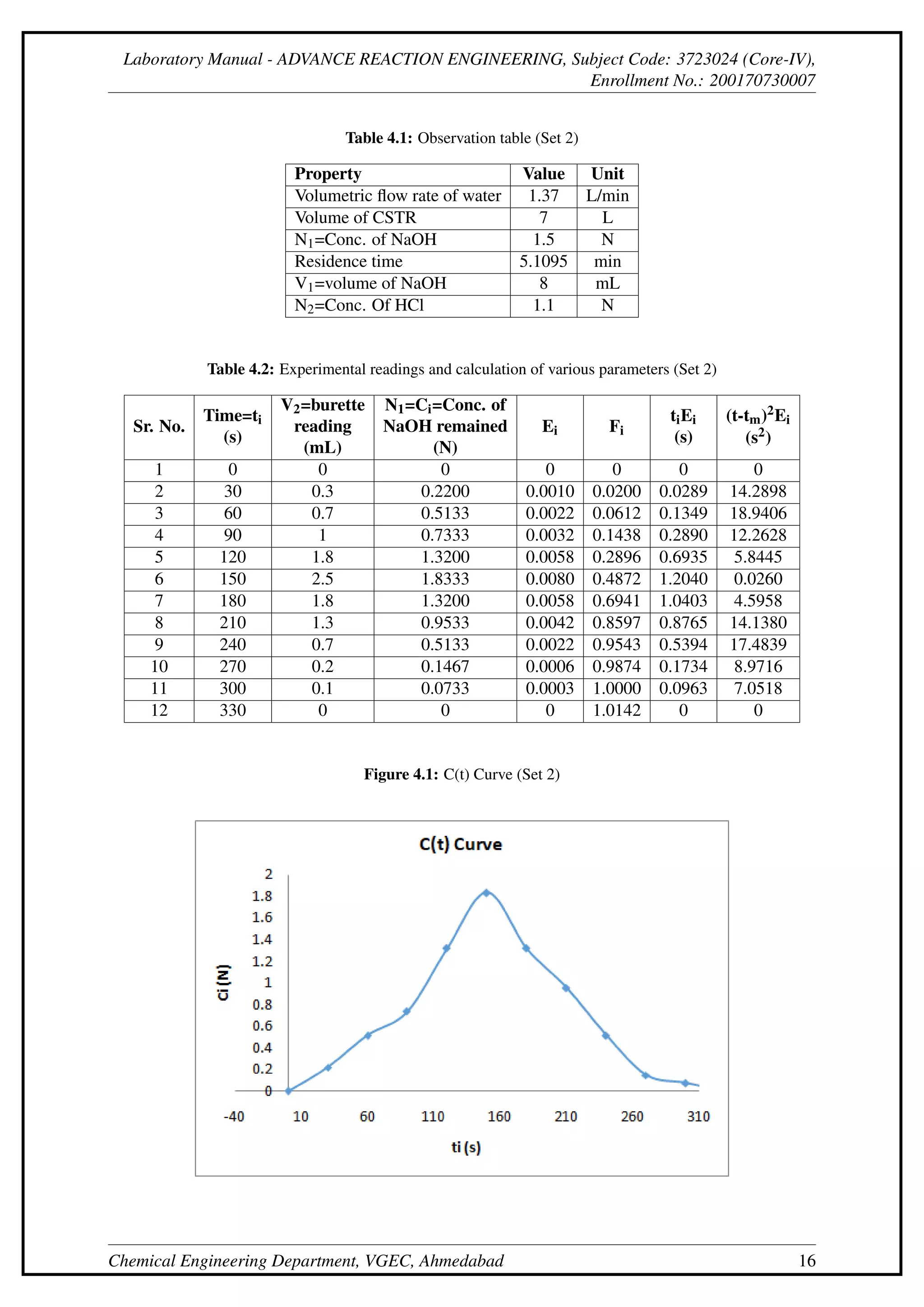
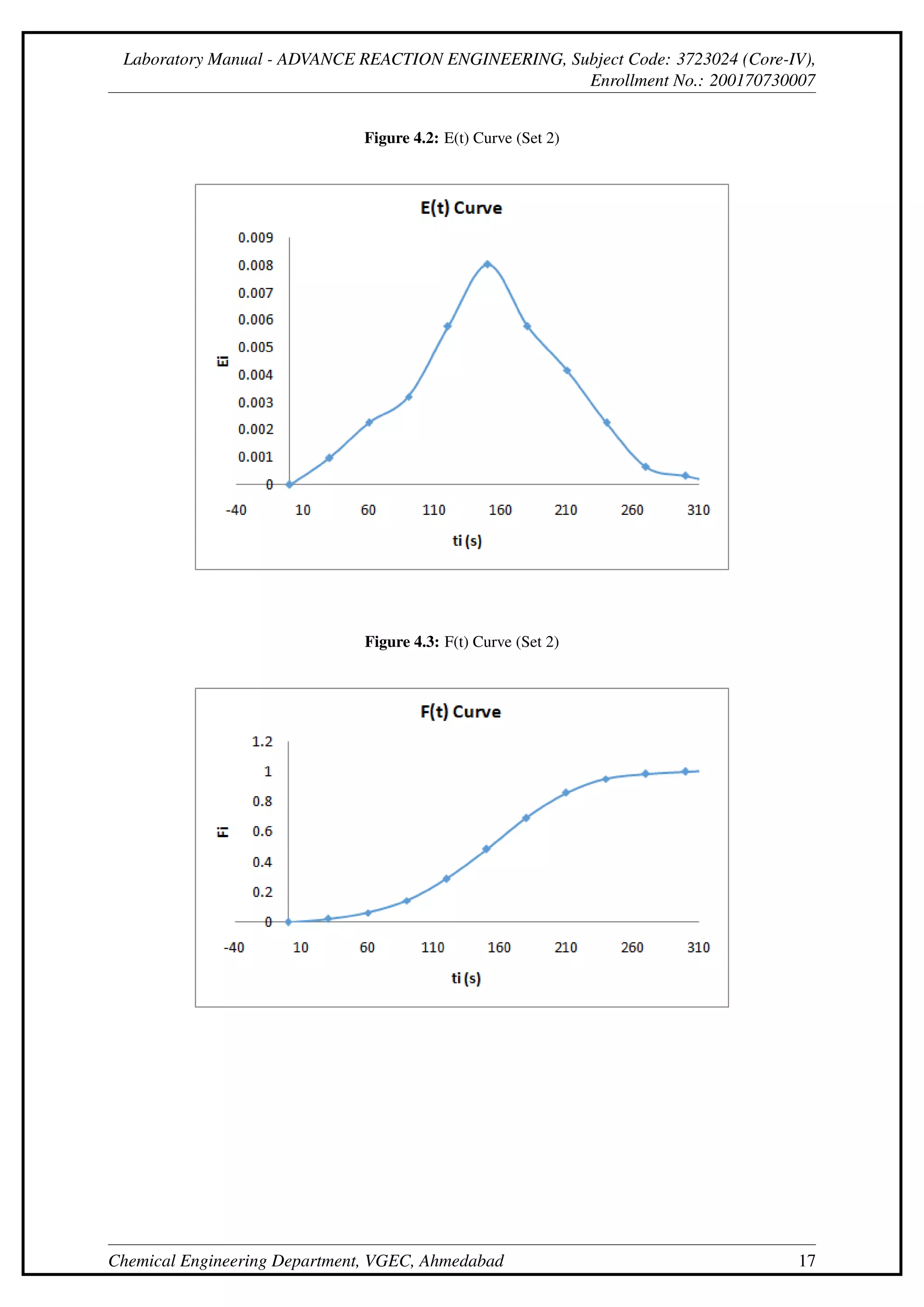
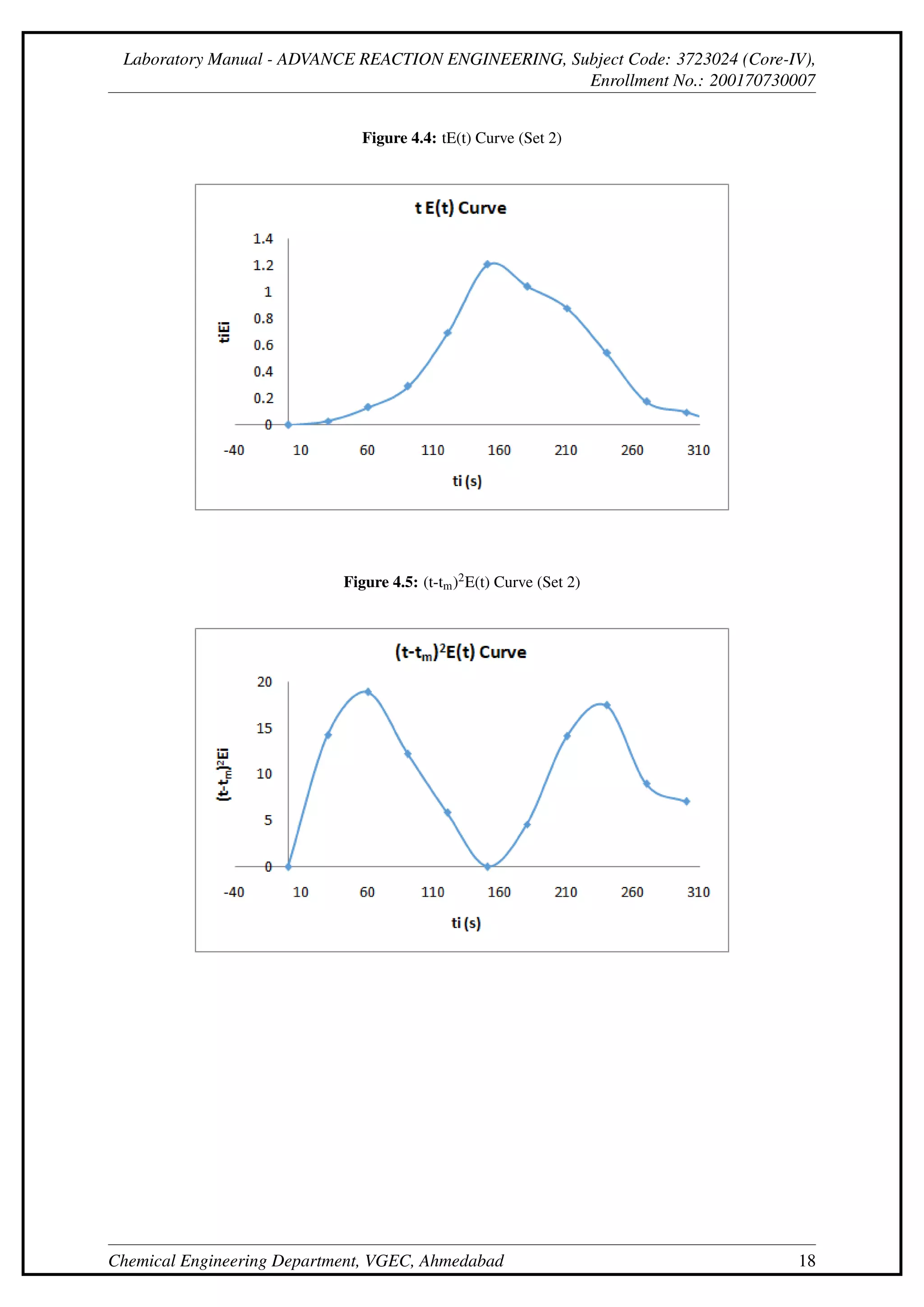
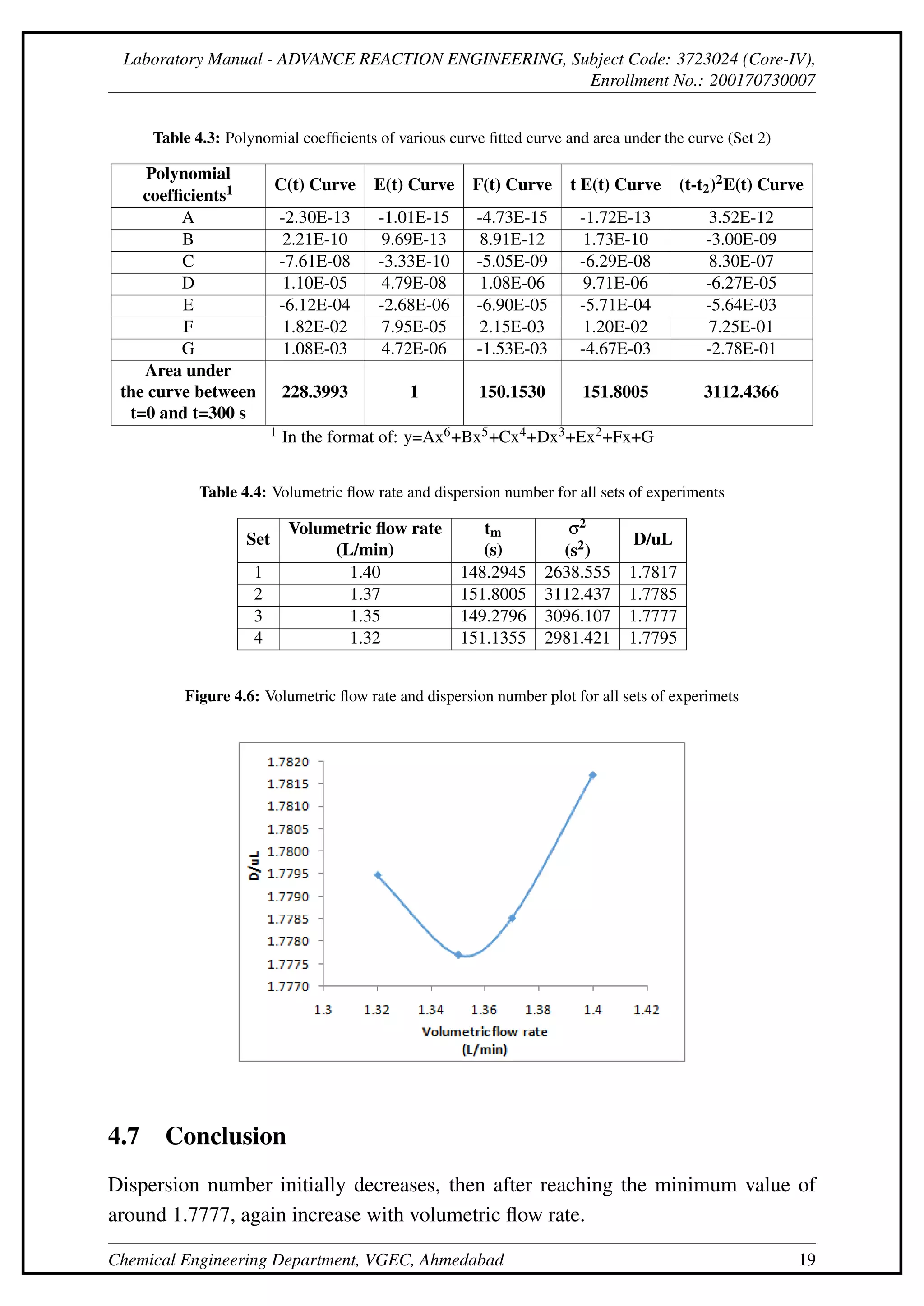
Laboratory Manual - ADVANCE REACTION ENGINEERING, Subject Code: 3723024 (Core-IV),
Enrollment No.: 200170730007
Experiment No. 4
Residence Time Distribution for Continuous Flow Stirred Tank
Reactor (CSTR)
4.1 Objective
• To construct ‘C’ and ‘E’ curve for delta function input.
• To calculate the dispersion number for different flow rates.
4.2 Apparatus
1. One tubular flow reactor with inlet and outlet flow arrangement.
2. Tracer injection system
3. Stop watch and test tubes
4. Titration set
4.3 Chemical
1. Oxalic acid ((CO2H)2(aq)) 0.05 N
2. Sodium Hydroxide (NaOH(aq)) 0.5 N
3. Hydrochloric Acid (HCl(aq)) 0.1 N
4. Indicator: Phenolphthalein
Chemical Engineering Department, VGEC, Ahmedabad 13
Laboratory Manual - ADVANCE REACTION ENGINEERING, Subject Code: 3723024 (Core-IV),
Enrollment No.: 200170730007
4.4 Theory
According to the dispersion model; and by Fick’s law for molecular diffusion in x
direction the differential equation is
∂C
∂t
= D
∂2C
∂x2
Where, D = longitudinal or axial dispersion coefficient showing the degree of back
mixing during the flow. Introducing the dimensionless variables,
Z =
x
L
,θ =
t
t
= u
L
t
The basic differential equation becomes:
∂C
∂θ
=
D
uL
∂2C
∂z2
−
∂C
∂z
Where D/uL is called the dispersion number. For plug flow through reactor,
D
uL
→ 0
For mixed flow through reactor,
D
uL
→ ∞
The variance,
σ2
=
∑t2
i Ci
∑Ci
−t2 =
∑t2
i Ci
∑Ci
−

∑tiCi
∑Ci
2
For closed vessel (variance based on dimensionless time units)
σ2
θ =
σ2
t2
σ2
θ =
σ2
t2
= 2
D
uL
−2

D
uL
2 
1−e−uL
D

4.5 Procedure
1. Standardize the Sodium hydroxide (NaOH) and Hydrochloric acid (HCl) solu-
tions by using 0.05 N Oxalic acid solutions before titration.
2. Start the circulation of a fluid through CSTR and adjust the flow rate in range
of 200 cm2/min to 1000 cm2/min.
Chemical Engineering Department, VGEC, Ahmedabad 14
Laboratory Manual - ADVANCE REACTION ENGINEERING, Subject Code: 3723024 (Core-IV),
Enrollment No.: 200170730007
3. First inject the dummy tracer and see how long the dummy tracer molecule
stays within the reactor. Divide that time into equal time interval and then
inject 5 N Sodium Hydroxide (NaOH) and start the stopwatch. Collect the
sample at a regular time interval. Collect number of samples that cover a total
time period that spent by dummy tracer molecule within the reactor. Titrate the
sample against 0.1 N Hydrochloric acid (HCl)) solutions.
4. Repeat the same procedure for another 3 different flow rates.
4.6 Calculation
• First of all plot the graph of concentration C (t) versus time (t) and find out
R ∞
0 C(t)dt either trapezoidal method or Simpson 1/3 rule or Simpson 3/8 rule
or area under the curve. One another approach of curve fitting and integration
of the curve is also suitable.
• Calculation of E(t):
E(t) =
C(t)
R ∞
0 C(t)dt
• Calculation of F(t):
F(t) =
Z t
0
E(t)dt
• Calculation of tm:
tm =
Z ∞
0
tE(t)dt
• Calculation of σ2:
σ2
=
Z ∞
0
(t −tm)2
E(t)dt
• Calculation of D/uL:
σ2
t2
m
= 2
D
uL
−2

D
uL
2 
1−e−uL
D

Chemical Engineering Department, VGEC, Ahmedabad 15
Laboratory Manual - ADVANCE REACTION ENGINEERING, Subject Code: 3723024 (Core-IV),
Enrollment No.: 200170730007
Table 4.1: Observation table (Set 2)
Property Value Unit
Volumetric flow rate of water 1.37 L/min
Volume of CSTR 7 L
N1=Conc. of NaOH 1.5 N
Residence time 5.1095 min
V1=volume of NaOH 8 mL
N2=Conc. Of HCl 1.1 N
Table 4.2: Experimental readings and calculation of various parameters (Set 2)
Sr. No.
Time=ti
(s)
V2=burette
reading
(mL)
N1=Ci=Conc. of
NaOH remained
(N)
Ei Fi
tiEi
(s)
(t-tm)2Ei
(s2)
1 0 0 0 0 0 0 0
2 30 0.3 0.2200 0.0010 0.0200 0.0289 14.2898
3 60 0.7 0.5133 0.0022 0.0612 0.1349 18.9406
4 90 1 0.7333 0.0032 0.1438 0.2890 12.2628
5 120 1.8 1.3200 0.0058 0.2896 0.6935 5.8445
6 150 2.5 1.8333 0.0080 0.4872 1.2040 0.0260
7 180 1.8 1.3200 0.0058 0.6941 1.0403 4.5958
8 210 1.3 0.9533 0.0042 0.8597 0.8765 14.1380
9 240 0.7 0.5133 0.0022 0.9543 0.5394 17.4839
10 270 0.2 0.1467 0.0006 0.9874 0.1734 8.9716
11 300 0.1 0.0733 0.0003 1.0000 0.0963 7.0518
12 330 0 0 0 1.0142 0 0
Figure 4.1: C(t) Curve (Set 2)
Chemical Engineering Department, VGEC, Ahmedabad 16
Laboratory Manual - ADVANCE REACTION ENGINEERING, Subject Code: 3723024 (Core-IV),
Enrollment No.: 200170730007
Figure 4.2: E(t) Curve (Set 2)
Figure 4.3: F(t) Curve (Set 2)
Chemical Engineering Department, VGEC, Ahmedabad 17
Laboratory Manual - ADVANCE REACTION ENGINEERING, Subject Code: 3723024 (Core-IV),
Enrollment No.: 200170730007
Figure 4.4: tE(t) Curve (Set 2)
Figure 4.5: (t-tm)2E(t) Curve (Set 2)
Chemical Engineering Department, VGEC, Ahmedabad 18
Laboratory Manual - ADVANCE REACTION ENGINEERING, Subject Code: 3723024 (Core-IV),
Enrollment No.: 200170730007
Table 4.3: Polynomial coefficients of various curve fitted curve and area under the curve (Set 2)
Polynomial
coefficients1 C(t) Curve E(t) Curve F(t) Curve t E(t) Curve (t-t2)2E(t) Curve
A -2.30E-13 -1.01E-15 -4.73E-15 -1.72E-13 3.52E-12
B 2.21E-10 9.69E-13 8.91E-12 1.73E-10 -3.00E-09
C -7.61E-08 -3.33E-10 -5.05E-09 -6.29E-08 8.30E-07
D 1.10E-05 4.79E-08 1.08E-06 9.71E-06 -6.27E-05
E -6.12E-04 -2.68E-06 -6.90E-05 -5.71E-04 -5.64E-03
F 1.82E-02 7.95E-05 2.15E-03 1.20E-02 7.25E-01
G 1.08E-03 4.72E-06 -1.53E-03 -4.67E-03 -2.78E-01
Area under
the curve between
t=0 and t=300 s
228.3993 1 150.1530 151.8005 3112.4366
1 In the format of: y=Ax6+Bx5+Cx4+Dx3+Ex2+Fx+G
Table 4.4: Volumetric flow rate and dispersion number for all sets of experiments
Set
Volumetric flow rate
(L/min)
tm
(s)
σ2
(s2)
D/uL
1 1.40 148.2945 2638.555 1.7817
2 1.37 151.8005 3112.437 1.7785
3 1.35 149.2796 3096.107 1.7777
4 1.32 151.1355 2981.421 1.7795
Figure 4.6: Volumetric flow rate and dispersion number plot for all sets of experimets
4.7 Conclusion
Dispersion number initially decreases, then after reaching the minimum value of
around 1.7777, again increase with volumetric flow rate.
Chemical Engineering Department, VGEC, Ahmedabad 19
Laboratory Manual - ADVANCE REACTION ENGINEERING, Subject Code: 3723024 (Core-IV),
Enrollment No.: 200170730007
4.8 Quiz
4.8.1 Discuss the different types of input used for RTD study.
The two most used methods of injection are as follows:
• Step input
• Pulse input
• Cyclic input
• Random input
4.8.2 Write down the physical significance of dispersion number.
• Higher the value of dispersion co-efficient, smaller is the value of Peclet num-
ber and consequently the Rate of transport by Dispersion is high.
• Similarly, Lower the value of Dispersion co-efficient, larger is the value of
Peclet number and consequently the Rate of transport by Dispersion is low.
4.8.3 What is mean by D/u L → 0?
• The amount of axial mixing is zero, like in case of an ideal PFR.
4.8.4 What is the molecularity of the reaction: H2 + Br2 → 2HBr?
• Molecularity: 2
• Order: 3/2
Chemical Engineering Department, VGEC, Ahmedabad 20

Laboratory_Manual_ARE EXP 4 1.pdf

  • 1.
    Laboratory Manual -ADVANCE REACTION ENGINEERING, Subject Code: 3723024 (Core-IV), Enrollment No.: 200170730007 Experiment No. 4 Residence Time Distribution for Continuous Flow Stirred Tank Reactor (CSTR) 4.1 Objective • To construct ‘C’ and ‘E’ curve for delta function input. • To calculate the dispersion number for different flow rates. 4.2 Apparatus 1. One tubular flow reactor with inlet and outlet flow arrangement. 2. Tracer injection system 3. Stop watch and test tubes 4. Titration set 4.3 Chemical 1. Oxalic acid ((CO2H)2(aq)) 0.05 N 2. Sodium Hydroxide (NaOH(aq)) 0.5 N 3. Hydrochloric Acid (HCl(aq)) 0.1 N 4. Indicator: Phenolphthalein Chemical Engineering Department, VGEC, Ahmedabad 13
  • 2.
    Laboratory Manual -ADVANCE REACTION ENGINEERING, Subject Code: 3723024 (Core-IV), Enrollment No.: 200170730007 4.4 Theory According to the dispersion model; and by Fick’s law for molecular diffusion in x direction the differential equation is ∂C ∂t = D ∂2C ∂x2 Where, D = longitudinal or axial dispersion coefficient showing the degree of back mixing during the flow. Introducing the dimensionless variables, Z = x L ,θ = t t = u L t The basic differential equation becomes: ∂C ∂θ = D uL ∂2C ∂z2 − ∂C ∂z Where D/uL is called the dispersion number. For plug flow through reactor, D uL → 0 For mixed flow through reactor, D uL → ∞ The variance, σ2 = ∑t2 i Ci ∑Ci −t2 = ∑t2 i Ci ∑Ci − ∑tiCi ∑Ci 2 For closed vessel (variance based on dimensionless time units) σ2 θ = σ2 t2 σ2 θ = σ2 t2 = 2 D uL −2 D uL 2 1−e−uL D 4.5 Procedure 1. Standardize the Sodium hydroxide (NaOH) and Hydrochloric acid (HCl) solu- tions by using 0.05 N Oxalic acid solutions before titration. 2. Start the circulation of a fluid through CSTR and adjust the flow rate in range of 200 cm2/min to 1000 cm2/min. Chemical Engineering Department, VGEC, Ahmedabad 14
  • 3.
    Laboratory Manual -ADVANCE REACTION ENGINEERING, Subject Code: 3723024 (Core-IV), Enrollment No.: 200170730007 3. First inject the dummy tracer and see how long the dummy tracer molecule stays within the reactor. Divide that time into equal time interval and then inject 5 N Sodium Hydroxide (NaOH) and start the stopwatch. Collect the sample at a regular time interval. Collect number of samples that cover a total time period that spent by dummy tracer molecule within the reactor. Titrate the sample against 0.1 N Hydrochloric acid (HCl)) solutions. 4. Repeat the same procedure for another 3 different flow rates. 4.6 Calculation • First of all plot the graph of concentration C (t) versus time (t) and find out R ∞ 0 C(t)dt either trapezoidal method or Simpson 1/3 rule or Simpson 3/8 rule or area under the curve. One another approach of curve fitting and integration of the curve is also suitable. • Calculation of E(t): E(t) = C(t) R ∞ 0 C(t)dt • Calculation of F(t): F(t) = Z t 0 E(t)dt • Calculation of tm: tm = Z ∞ 0 tE(t)dt • Calculation of σ2: σ2 = Z ∞ 0 (t −tm)2 E(t)dt • Calculation of D/uL: σ2 t2 m = 2 D uL −2 D uL 2 1−e−uL D Chemical Engineering Department, VGEC, Ahmedabad 15
  • 4.
    Laboratory Manual -ADVANCE REACTION ENGINEERING, Subject Code: 3723024 (Core-IV), Enrollment No.: 200170730007 Table 4.1: Observation table (Set 2) Property Value Unit Volumetric flow rate of water 1.37 L/min Volume of CSTR 7 L N1=Conc. of NaOH 1.5 N Residence time 5.1095 min V1=volume of NaOH 8 mL N2=Conc. Of HCl 1.1 N Table 4.2: Experimental readings and calculation of various parameters (Set 2) Sr. No. Time=ti (s) V2=burette reading (mL) N1=Ci=Conc. of NaOH remained (N) Ei Fi tiEi (s) (t-tm)2Ei (s2) 1 0 0 0 0 0 0 0 2 30 0.3 0.2200 0.0010 0.0200 0.0289 14.2898 3 60 0.7 0.5133 0.0022 0.0612 0.1349 18.9406 4 90 1 0.7333 0.0032 0.1438 0.2890 12.2628 5 120 1.8 1.3200 0.0058 0.2896 0.6935 5.8445 6 150 2.5 1.8333 0.0080 0.4872 1.2040 0.0260 7 180 1.8 1.3200 0.0058 0.6941 1.0403 4.5958 8 210 1.3 0.9533 0.0042 0.8597 0.8765 14.1380 9 240 0.7 0.5133 0.0022 0.9543 0.5394 17.4839 10 270 0.2 0.1467 0.0006 0.9874 0.1734 8.9716 11 300 0.1 0.0733 0.0003 1.0000 0.0963 7.0518 12 330 0 0 0 1.0142 0 0 Figure 4.1: C(t) Curve (Set 2) Chemical Engineering Department, VGEC, Ahmedabad 16
  • 5.
    Laboratory Manual -ADVANCE REACTION ENGINEERING, Subject Code: 3723024 (Core-IV), Enrollment No.: 200170730007 Figure 4.2: E(t) Curve (Set 2) Figure 4.3: F(t) Curve (Set 2) Chemical Engineering Department, VGEC, Ahmedabad 17
  • 6.
    Laboratory Manual -ADVANCE REACTION ENGINEERING, Subject Code: 3723024 (Core-IV), Enrollment No.: 200170730007 Figure 4.4: tE(t) Curve (Set 2) Figure 4.5: (t-tm)2E(t) Curve (Set 2) Chemical Engineering Department, VGEC, Ahmedabad 18
  • 7.
    Laboratory Manual -ADVANCE REACTION ENGINEERING, Subject Code: 3723024 (Core-IV), Enrollment No.: 200170730007 Table 4.3: Polynomial coefficients of various curve fitted curve and area under the curve (Set 2) Polynomial coefficients1 C(t) Curve E(t) Curve F(t) Curve t E(t) Curve (t-t2)2E(t) Curve A -2.30E-13 -1.01E-15 -4.73E-15 -1.72E-13 3.52E-12 B 2.21E-10 9.69E-13 8.91E-12 1.73E-10 -3.00E-09 C -7.61E-08 -3.33E-10 -5.05E-09 -6.29E-08 8.30E-07 D 1.10E-05 4.79E-08 1.08E-06 9.71E-06 -6.27E-05 E -6.12E-04 -2.68E-06 -6.90E-05 -5.71E-04 -5.64E-03 F 1.82E-02 7.95E-05 2.15E-03 1.20E-02 7.25E-01 G 1.08E-03 4.72E-06 -1.53E-03 -4.67E-03 -2.78E-01 Area under the curve between t=0 and t=300 s 228.3993 1 150.1530 151.8005 3112.4366 1 In the format of: y=Ax6+Bx5+Cx4+Dx3+Ex2+Fx+G Table 4.4: Volumetric flow rate and dispersion number for all sets of experiments Set Volumetric flow rate (L/min) tm (s) σ2 (s2) D/uL 1 1.40 148.2945 2638.555 1.7817 2 1.37 151.8005 3112.437 1.7785 3 1.35 149.2796 3096.107 1.7777 4 1.32 151.1355 2981.421 1.7795 Figure 4.6: Volumetric flow rate and dispersion number plot for all sets of experimets 4.7 Conclusion Dispersion number initially decreases, then after reaching the minimum value of around 1.7777, again increase with volumetric flow rate. Chemical Engineering Department, VGEC, Ahmedabad 19
  • 8.
    Laboratory Manual -ADVANCE REACTION ENGINEERING, Subject Code: 3723024 (Core-IV), Enrollment No.: 200170730007 4.8 Quiz 4.8.1 Discuss the different types of input used for RTD study. The two most used methods of injection are as follows: • Step input • Pulse input • Cyclic input • Random input 4.8.2 Write down the physical significance of dispersion number. • Higher the value of dispersion co-efficient, smaller is the value of Peclet num- ber and consequently the Rate of transport by Dispersion is high. • Similarly, Lower the value of Dispersion co-efficient, larger is the value of Peclet number and consequently the Rate of transport by Dispersion is low. 4.8.3 What is mean by D/u L → 0? • The amount of axial mixing is zero, like in case of an ideal PFR. 4.8.4 What is the molecularity of the reaction: H2 + Br2 → 2HBr? • Molecularity: 2 • Order: 3/2 Chemical Engineering Department, VGEC, Ahmedabad 20