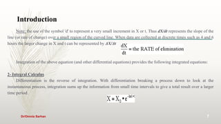
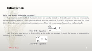
This document discusses pharmacokinetics and provides information about key concepts used in pharmacokinetics including: - Logarithms and how they relate to calculating drug concentrations over time - Differential and integral calculus which are used to develop equations to model rates of change in drug absorption and elimination over small time intervals - How to write differential equations to model different rate processes like zero-order, first-order, and Michaelis-Menten kinetics - 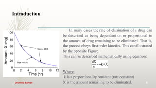The use of graphs including Cartesian and semi-log scales to plot drug concentration vs. time profiles - Examples of using these concepts to solve pharmacokinetic problems

1. Dr/Omnia Sarhan 1
PHARMACOKINETICS
Lecture 5

2. Dr/Omnia Sarhan
‫الكليـــــــــــــة‬ ‫رؤيــــــــــــة‬
‫الكليــــــــــــة‬ ‫رســـــــــــــــالة‬
‫الريادة‬
ً
‫محليا‬
ً
‫واقليميا‬
ً
‫ودوليا‬
‫لالرتقاء‬
‫بصحة‬
‫االنسان‬
‫من‬
‫خالل‬
‫استخدا‬
‫م‬
‫االبتكارات‬
‫فى‬
‫مجال‬
‫التعليم‬
‫والبحوث‬
‫العلمية‬
‫والممارسات‬
‫التطبيقية‬
.
‫توفير‬
‫أفضل‬
‫الممارسات‬
‫في‬
‫مجال‬
‫التعليم‬
‫والتعلم‬
‫والتدريب‬
‫وإستمرارية‬
‫خ‬
‫لق‬
‫فرص‬
‫للطالب‬
‫والخريجين‬
‫بإبتكار‬
‫ونشر‬
‫وتطبيق‬
‫المعرفة‬
‫الحديثة‬
‫المرتكزة‬
‫على‬
‫البحوث‬
‫والتطبيقات‬
‫في‬
‫العلوم‬
‫الصيدلية‬
‫واإلكلينيكية‬
‫واإلجتماعية‬
‫للنهوض‬
‫بال‬
‫صحة‬

3. Dr/Omnia Sarhan
3
Upon successful completion of this course the student should be able to;
• Describe the physicochemical and physiological factors that influence the
absorption of drugs
from extra and intravascular routs of administration, their distribution within the
body, and their
routes and mechanisms of elimination
• Explain how dose, bioavailability, rate of absorption, apparent volume of
distribution, total
clearance, and elimination half-life affect the plasma concentrations of a drug after
administration of single oral or single IV bolus dose
• Describe the factors which determine the time-course of systemic accumulation of
a drug
administered by multiple oral, multiple IV bolus and continuous infusion doses
• Differentiate between linear and non-linear pharmacokinetic models

4. Introduction
Dr/Omnia Sarhan 4
I- Logarithm
The logarithm of a number is the exponent or power to which a given base number must be raised to equal
that number. Thus, the logarithm of Y to the base, b, equals X, or log b (Y) = X. The logarithm of 0 and all
negative numbers is undefined or nonexistent. The logarithm of 1 is 0 and of numbers <1 is negative in all
systems.
The relationships between common and natural logarithms are the following:
a. log Y = ln Y/ln 10 = ln Y/2.303
b. ln Y = ln 10 × log Y = 2.303 × log Y

5. Introduction
Dr/Omnia Sarhan 5
II- Calculus
1- Differential Calculus
Pharmacokinetics is the study of the rate of drug absorption and disposition in the body. Thus differential calculus
is an important stepping stone in the development of many of the equations used.
Differential calculus is involved with the study of rates of processes. The calculus part comes in when we look at
these processes in detail, that is, during small time intervals. We may say that at time zero a patient has a concentration
of 25 mg/l of a drug in plasma and at time 24 hours the concentration is 5 mg/l. That may be interesting in itself, but it
doesn't give us any idea of the concentration between 0 and 24 hours, or after 24 hours. Using differential calculus we
are able to develop equations to look at the process during the small time intervals that make up the total time interval
of 0 to 24 hours.

6. Introduction
Dr/Omnia Sarhan 6
In many cases the rate of elimination of a drug can
be described as being dependent on or proportional to
the amount of drug remaining to be eliminated. That is,
the process obeys first order kinetics. This can illustrated
by the opposite Figure.
This can be described mathematically using equation:
Where:
k is a proportionality constant (rate constant)
X is the amount remaining to be eliminated.

7. Introduction
Dr/Omnia Sarhan 7
Note: the use of the symbol 'd' to represent a very small increment in X or t. Thus dX/dt represents the slope of the
line (or rate of change) over a small region of the curved line. When data are collected at discrete times such as 4 and 6
hours the larger change in X and t can be represented by ΔX/Δt
Integration of the above equation (and other differential equations) provides the following integrated equations:
2- Integral Calculus
Differentiation is the reverse of integration. With differentiation breaking a process down to look at the
instantaneous process, integration sums up the information from small time intervals to give a total result over a larger
time period.

8. Introduction
Dr/Omnia Sarhan 8
First: How writing differential equations?
Rate processes in the field of pharmacokinetics are usually limited to first order, zero order and occasionally
Michaelis-Menten kinetics. Linear pharmacokinetic systems consist of first order disposition processes and bolus
doses, first order or zero order absorption rate processes. These rate processes can be described mathematically.
First Order Equation
Each first order rate process is described by a first order rate constant (k1) and the amount or concentration
remaining to be transferred (X1).
Zero Order Equation

9. Introduction
Dr/Omnia Sarhan 9
Zero order rate processes are described by the rate constant alone.
Michaelis Menten Equation
The Michaelis Menten process is somewhat more complicated with a maximum rate (velocity, Vm) and a
Michaelis constant (Km) and the amount or concentration remaining.
The full differential equation for any component of a pharmacokinetic model can be constructed by adding an
equation segment for each arrow in the pharmacokinetic model.
The rules for each segment:
1- Direction of the arrow
*If the arrow goes into the component the equation segment is positive
*If the arrow leaves the component the equation segment is negative.

10. Introduction
Dr/Omnia Sarhan 10
2- Type of rate process
*If the rate process is first order multiply the (first order) rate constant by the amount or
concentration of drug in the component at the tail of the arrow.
*If the process is zero order just enter the rate constant.

11. Introduction
Dr/Omnia Sarhan 11
Component 1 There is one arrow leading out of component one so the rate process is negative.
This process is zero order so we just write the rate constant. The equation for this component is:
Component 2 This component is more of a challenge. There are three arrows connected with this
component. One arrow leads to the compartment so this equation segment is positive. The other
two arrows lead away from the component and these equation segments are negative. Starting
with the zero order process provides is a positive k0 to the differential equation. The first order
process is developed as the rate constant multiplied by the amount remaining in component 2.
This is negative and is -k1  X2. The final segment is the Michaelis Menten process from
component 2 to component 4. This is also negative and is described as -Vm x X2 / (Km + X2).
The total differential equation for this component is:

12. Introduction
Dr/Omnia Sarhan 12
Component 3 OK; downhill from here. Now we have one arrow going to this component from
component 2, thus the equation segment is positive. The rate process is first order so we multiply the
rate constant by the amount remaining in the component at the tail of the arrow, component 2. The
equation is:
Component 4 The fourth component is also described with one equation segment. The arrow leads to
this component so the segment is positive. The rate process is a Michaelis Menten process. The
equation for this component is:

13. Introduction
Dr/Omnia Sarhan 13
GRAPHS
Graphs are usually used to present the relationship between two or more variables. In pharmacokinetics, graphs
are commonly utilized to represent the drug concentration in the systemic circulation or drug pharmacological effect as
a function of time after drug administration. In the two-dimensional graphs that are commonly used in
pharmacokinetics, the drug concentration or drug effect (the dependent variable) is plotted on the y-axis, while time
(the independent variable) is plotted on the x-axis. There are two types of scales that are commonly utilized in
pharmacokinetics, the Cartesian scale and the semilog scale.
1- Cartesian Scale
In the Cartesian scale, both the y-axis and the x-axis are linear. Each point can be plotted on the Cartesian scale by
a pair of numerical coordinates that determine the perpendicular distance of the point from the x-axis and the y-axis.

14. Introduction
Dr/Omnia Sarhan 14
Although negative or positive values can be used for the coordinates in the
Cartesian scale, only positive coordinate values are used to present plasma
concentration versus time profile. The opposite Figure is an example of the
Cartesian scale.
2- Semilog Scale
The semilog scale has a logarithmic scale on the y-axis and a linear scale on
the x-axis, as in the next Figure. This type of graph is useful in plotting values
that are changing exponentially. On the semilog graph the spacing of the scale on
the y-axis is proportional to the logarithm of the number, not the number itself.
Plotting data on the semilog scale is equivalent of converting the dependent
variable values to their

15. Introduction
Dr/Omnia Sarhan 15
log values, and plotting the data on the
linear scale. The semilog graph paper
consists of repeated units called cycles.
Each of these cycles covers a single log10
unit, or 10-fold increase in number. The
semilog graph paper is available in one,
two, three, or more cycles per sheet.
Example
Plot the following drug concentration–
time data on the semilog scale:

16. Introduction
Dr/Omnia Sarhan 16
Answer
• The scale on the x-axis is chosen to make the time
points cover the largest portion of the x-axis.
• The drug concentration values are used to determine the
number of cycles needed.
Three cycles are needed to plot these values.

17. Problems
Dr/Omnia Sarhan 17
1-The linear relationship that describes the change in the drug amount (A) in mg, as a
function of time (t) in h, can be described by the following equation: A = 120 mg − 2
(mg/h) t.
a. Calculate the amount of the drug remaining after 10 h.
b. What is the time required for the drug amount to decrease to zero?

18. Problems
Dr/Omnia Sarhan
18
2- In an experiment to study the chemical decomposition, a drug solution was prepared and an aliquot of the
drug solution was obtained at different time points. The drug concentrations in the samples and the results
were as follows:
a. Draw the drug concentration against time on the Cartesian scale and graphically estimate the slope and y-
intercept.
b. Write the equation that describes the change in drug concentration with time.

19. Introduction
19
Rates and order of reactions
Rates
Is the velocity within which the reaction occurs. Consider the following reaction:
Drug A drug B
The amount of drug A is decreasing with respect to time
So Rate = - dA / dt (forward reaction)
Or
since the amount of B increases with respect to time
Rate = + dB / dt
The order of a reaction
Refers to the actual manner in which the concentration of the drug tends to influence the rate of
reaction or process. If the drug A changed to B and the concentration of A is C, the rate of change of A
to B as a function of time will expressed as
Dr/Omnia Sarhan

20. a +ve rate means that the concen. is increasing with time
(product).
a -ve rate means that the concentration is falling with time
(reactant).
Dr/ Omnia Sarhan

21. Introduction
21
dC / dt = - K Cn
Where;
dC / dt = the rate of reaction
K = rate constant
n = the order of the reaction or process.
When n = zero, it is called zero order reaction, when n = 1, it is called first order reaction, and so on.
1- Zero order kinetics (constant rate process);
Constant rate change and the change is independent on the concentration of the drug. It is not
possible to increase the rate of process by increasing the concentration of the drug. An example is the
elimination of alcohol. Drugs that show this type of elimination will show accumulation of plasma
levels of the drug and hence nonlinear pharmacokinetics.
Dr/Omnia Sarhan

22. Introduction
22
The amount of the drug (A) is decreasing at a constant time interval (t)
A = - Ko t + Ao
Where Ao = the amount of the drug at time = zero
A = the amount of the drug at time = t
Dr/Omnia Sarhan

23. Zero-Order Reaction
Graphically on cartesian paper:
t
k
C
Ct 0
0 

23
Time
Ct
C0
Slope=-k0
t
k
C
Ct 0
0 

Dr/Omnia Sarhan

24. – Equation of straight line:
– y = ax + b
– (a: slope, b: intercept)
x
y
Intercept
= b
Slope = a
kt
C
Ct 
 0
24
Dr/Omnia Sarhan

25. Introduction
25
The half-life (t ½);
Expresses the period of time required for the amount or concentration of a drug to decrease by one
half. Or the time required for the plasma concentration to drop from its initial value to the half. i.e.,
when t = t ½ , A = Ao / 2 .
t ½ for zero order reaction;
A = - Ko t + Ao
When t = t ½, A = Ao / 2
t ½ = Ao / 2 Ko
e.g., for zero order delivery
1. Sustained release
2. I.V infusion
3. Trans-dermal preparations
Dr/Omnia Sarhan

26. Half-life of Zero-order Reactions
0
0
2
/
1
2k
C
t 
t
k
C
Ct 0
0 

When one half-life has elapsed, by definition
2
/
1
0
0
0
2
t
k
C
C


2
0
C
Ct 
2
0
0
2
/
1
0
C
C
t
k 

2
0
2
/
1
0
C
t
k 
Dr/ Omnia Sarhan

27. 0
0
2
/
1
2k
C
t 
– Half life of zero order reaction is directly proportional to
initial concentration.
– Thus half life decrease as reaction proceed with time
(when C0 is reduced by a factor of 2, the half-life is also
decreased by a factor of 2 (in fact each successive half-
life is half the preceding one)
100%A
10 min
50%A 25%A 12.5%A
5 min 2.5 min
27
Dr/Omnia Sarhan

28. Expiration Date
It is the date at which 10% drug concentration is decomposed
(increase toxicity & decrease activity).
k
C
t
10
0
90 
%
90
0
0
9
.
0 t
k
C
C 

0
9
.
0 C
Ct 
0
0
%
90 9
.
0 C
C
kt 
 0
90 1
.
0 C
t
k 
Dr/ Omnia Sarhan

29. A drug product has an initial concentration of 125 mg/ml decays by
zero order kinetics, (k=0.5 mg/ml/hr). What is the concentration of the
intact drug remaining after 3 days? When the drug reaches zero
concentration?
Answer:
C = Co – Kt
C = 125 - 0.5 * (3 x 24)
C = 89 mg / ml
C = Co – Kt
0 = 125 – 0.5*t
t = 250 hour
Example 1
29
Dr/Omnia Sarhan

30. t
C
C
k t
o 

1
.
/
00052
.
473
0.225
-
0.47
k 


 days
liter
mole
months
days
K
C
t o
15
452
00052
.
0
2
47
.
0
2
2
/
1 




The decomposition of multi-sulfa compound was found to follow zero order
kinetics. If its concentration was 0.47 mole/liter, when freshly prepared, and
after 473 days its concentration reached 0.225 mole/liter, calculate the
degradation rate constant and t1/2 .
Answer:
Example 2
kt
C
Ct 
 0
30
Dr/Omnia Sarhan

31. 300 240
10
6
 
  
o t
C C
k
t

  
90%
0.1 0.1 300
3
10
o
C
t
K
The degradation of a drug product follows zero order process. If the
Concentration was 300 units/ml when freshly prepared & after 6
Months, its concentration reached 240 units/ml. Calculate the Constant
of reaction and the shelf life of the product.
Answer:
units/ml/month
months
Example 3
kt
C
Ct 
 0
Dr/ Omnia Sarhan

32. Introduction
32
2- First order kinetics (linear kinetics)
The rate of reaction is directly proportional to the concentration. i.e., the change depends on the
concentration.
ln A – ln Ao = - k t
ln (A/Ao) = - k t
A /Ao = e-Kt………….. (1)
Where e is the natural logarithm, the equation has one exponent and called monoexponential rate
process.
Since ln = 2.303 log, equation 1 can be written as;
Log A = log Ao – k t / 2.303 ............ (2)
A plot of log A versus time, a straight line is obtained whose
slope = k / 2.303
intercept = log Ao
Dr/Omnia Sarhan

33. Introduction
33
T½ for first order reaction
t ½ =0.693/ k
Dr/Omnia Sarhan

34. Graphically on
semilog paper
Co
1
2
1
2 log
log
t
t
y
y
slope



34
Dr/Omnia Sarhan

35. v
Conc.
Time
100
1
90
2
14
3
9
4
4.2
5
0.08
6
35
Dr/Omnia Sarhan

36. %
Remaining
Time
C0
Slope = -k/2.303
= (log y2 – log y1) / (x2 – x1)
No zero on y axis
36
Dr/Omnia Sarhan

37. k
t
693
.
0
2
/
1 
Half life t1/2 is constant
& doesn’t depend on
concentration.
2
log
303
.
2
2
/
1
k
t 
303
.
2
log
log 0
kt
C
Ct 

303
.
2
log
2
/
1
log 2
/
1
0
0
kt
C
C 

0
0
2
/
1
2
1
log
303
.
2
C
C
k
t 
0
0
2
/
1
2
/
1
log
log
303
.
2
C
C
kt


0
0
2
/
1
2
/
1
log
303
.
2 C
C
kt

37
Dr/Omnia Sarhan

38. 100%A
10
min
50%
A
25%
A
12.5%
A
10
min
10
min
Half life t1/2 is constant
& doesn’t depend on
concentration.
38
Dr/Omnia Sarhan

39. ln ln o
c c kt
  
 
 
ln ln5 0.0005 120
ln 1.549 ln
4.71 /
C
C shift
C mg ml
  


90%
0.105 0.105
210
0.0005
t
k
  
Don’t forget to
check the units of
the problem
An ophthalmic solution dispensed at 5 mg/ml conc. exhibits a first order
reaction, with a rate constant of 0.0005 day-1. How much drug remaining
after 120 days? & how long will it take for the drug to degrade to 90% of its
initial concentration?
Answer:
A first order reaction
days
Example 1
39
Dr/Omnia Sarhan

40. The original concentration of one sample was 50 mg/ml. When assayed
20 months later the concentration was found to be 40 mg/ml, assuming
that the decomposition is first order, What is the half-life of this
product?
Ans.:
Co= 50mg/mL Ct= 40mg/mL t= 20 mon.
log Ct= log Co- Kt/2.303
log 40= log 50- 20K/2.303
K= 0.0111mon-1
T1/2= 0.693/K= 0.693/ 0.0111= 62.43 mon.
Example 2
40
Dr/Omnia Sarhan

41. 1/ 2
0.693 0.693
0.1215
5.7
k
t
  
At 25 °C, the half-life period for the decomposition of N205 is 5.7
hours and is independent of the initial pressure of N205,
calculate:
a- The time for the completion of the reaction.
b- The specific rate constant for the reaction.
Answer:
•t1/2 is independent on the initial conc. So, it is 1st order, hence the
reaction never goes to an end and the life time (time for completion
of the reaction) is infinity.
hr-1
Example 3
41
Dr/Omnia Sarhan

42. Intercept
Slope
(x-
axis)
(y-axis)
Half-life
eqn.
Integrated
rate eqn.
Orde
r
Co
-Ko
t
C
t1/2 = Co
2k
Co – C = kt
0
Log Co
-K
2.303
t
LogC
t1/2 = 0.693
k
1
303
.
2
log
log 0
kt
C
Ct 

Dr/Omnia Sarhan

43. Dr/Omnia Sarhan 43