Kdd 2009
•
1 like•602 views

The document analyzes the KDD Cup 2009 competition, which involved predicting customer behavior using a large customer database from Orange, a French telecommunications company. The competition attracted over 450 participants from 46 countries. Ensemble methods such as decision trees were very effective at handling the large dataset that had many samples, attributes, mixed variable types, and missing values. The top-performing models were able to rapidly build predictive models and score new entries on the large, noisy, and unbalanced customer database.

Recommended
Recommended
More Related Content
Similar to Kdd 2009
Similar to Kdd 2009 (20)
More from Houw Liong The
More from Houw Liong The (20)
Recently uploaded
Recently uploaded (20)
Kdd 2009
- 1. JMLR: Workshop and Conference Proceedings 7: 1-22 KDD cup 2009 Analysis of the KDD Cup 2009: Fast Scoring on a Large Orange Customer Database Isabelle Guyon isabelle@clopinet.com Clopinet, Berkeley, CA 94798, USA Vincent Lemaire vincent.lemaire@orange-ftgroup.com Orange Labs, Lannion, 22300, France Marc Boull´ e marc.boulle@orange-ftgroup.com Orange Labs, Lannion, 22300, France Gideon Dror gideon@mta.ac.il Academic College of Tel-Aviv-Yaffo, Tel Aviv 61083, Israel David Vogel dvogel@dataminingsolutions.net Data Mining Solutions, Orlando, Florida, USA Editor: Neil Lawrence Abstract We organized the KDD cup 2009 around a marketing problem with the goal of identifying data mining techniques capable of rapidly building predictive models and scoring new entries on a large database. Customer Relationship Management (CRM) is a key element of modern marketing strategies. The KDD Cup 2009 offered the opportunity to work on large marketing databases from the French Telecom company Orange to predict the propensity of customers to switch provider (churn), buy new products or services (appetency), or buy upgrades or add-ons proposed to them to make the sale more profitable (up-selling). The challenge started on March 10, 2009 and ended on May 11, 2009. This challenge attracted over 450 participants from 46 countries. We attribute the popularity of the challenge to several factors: (1) A generic problem relevant to the Industry (a classification problem), but presenting a number of scientific and technical challenges of practical interest including: a large number of training examples (50,000) with a large number of missing values (about 60%) and a large number of features (15,000), unbalanced class proportions (fewer than 10% of the examples of the positive class), noisy data, presence of categorical variables with many different values. (2) Prizes (Orange offered 10,000 Euros in prizes). (3) A well designed protocol and web site (we benefitted from past experience). (4) An effective advertising campaign using mailings and a teleconference to answer potential participants questions. The results of the challenge were discussed at the KDD conference (June 28, 2009). The principal conclusions are that ensemble methods are very effective and that ensemble of decision trees offer off-the-shelf solutions to problems with large numbers of samples and attributes, mixed types of variables, and lots of missing values. The data and the platform of the challenge remain available for research and educational purposes at http://www.kddcup-orange.com/. Keywords: challenge, classification, customer management, fast scoring c 2009 Isabelle Guyon, Vincent Lemaire, Marc Boull´, Gideon Dror, David Vogel. e
- 2. ´ Guyon, Lemaire, Boulle, Dror, Vogel 1. Introduction Customer Relationship Management (CRM) is a key element of modern marketing strategies. The KDD Cup 2009 offered the opportunity to work on large marketing databases from the French Telecom company Orange to predict the propensity of customers to switch provider (churn), buy new products or services (appetency), or buy upgrades or add-ons proposed to them to make the sale more profitable (up-selling). The most practical way to build knowledge on customers in a CRM system is to produce scores. A score (the output of a model) is an evaluation for all target variables to explain (i.e., churn, appetency or up-selling). Tools producing scores provide quantifiable information on a given population. The score is computed using customer records represented by a number of variables or features. Scores are then used by the information system (IS), for example, to personalize the customer relationship. The rapid and robust detection of the most predictive variables can be a key factor in a marketing application. An industrial customer analysis platform developed at Orange Labs, capable of building predictive models for datasets having a very large number of input variables (thousands) and instances (hundreds of thousands), is currently in use by Orange marketing. A key requirement is the complete automation of the whole process. The system extracts a large number of features from a relational database, selects a subset of informative variables and instances, and efficiently builds in a few hours an accurate classifier. When the models are deployed, the platform exploits sophisticated indexing structures and parallelization in order to compute the scores of millions of customers, using the best representation. The challenge was to beat the in-house system developed by Orange Labs. It was an opportunity for participants to prove that they could handle a very large database, including heterogeneous noisy data (numerical and categorical variables), and unbalanced class distributions. Time efficiency is often a crucial point. Therefore part of the competition was time-constrained to test the ability of the participants to deliver solutions quickly. The fast track of the challenge lasted five days only. To encourage participation, the slow track of the challenge allowed participants to continue working on the problem for an additional month. A smaller database was also provided to allow participants with limited computer resources to enter the challenge. 2. Background and motivations This challenge uses important marketing problems to benchmark classification methods in a setting, which is typical of large-scale industrial applications. A large database was made available by the French Telecom company, Orange with tens of thousands of examples and variables. This dataset is unusual in that it has a large number of variables making the problem particularly challenging to many state-of-the-art machine learning algorithms. The challenge participants were provided with masked customer records and their goal was to predict whether a customer will switch provider (churn), buy the main service (appetency) and/or buy additional extras (up-selling), hence solving three binary classification problems. Churn is the propensity of customers to switch between service providers, appetency is the propensity of customers to buy a service, and up-selling is the success in selling additional good or services to make a sale more profitable. Although the technical difficulty of scaling 2
- 3. Analysis of the KDD Cup 2009 up existing algorithms is the main emphasis of the challenge, the dataset proposed offers a variety of other difficulties: heterogeneous data (numerical and categorical variables), noisy data, unbalanced distributions of predictive variables, sparse target values (only 1 to 7 percent of the examples examples belong to the positive class) and many missing values. 3. Evaluation There is value in a CRM system to evaluate the propensity of customers to buy. Therefore, tools producing scores are more usable that tools producing binary classification results. The participants were asked to provide a score (a discriminant value or a posterior probability P (Y = 1|X)), and they were judged by the area under the ROC curve (AUC). The AUC is the area under the curve plotting sensitivity vs. (1− specificity) when the threshold θ is varied (or equivalently the area under the curve plotting sensitivity vs. specificity). We call “sensitivity” the error rate of the positive class and “specificity” the error rate of the negative class. The AUC is a standard metric in classification. There are several ways of estimating error bars for the AUC. We used a simple heuristic, which gives us approximate error bars, and is fast and easy to implement: we find on the AUC curve the point corresponding to the largest balanced accuracy BAC = 0.5 (sensitivity + specificity). We then estimate the standard deviation of the BAC as: σ= 1 2 p+ (1 − p+ ) p− (1 − p− ) + , m+ m− (1) where m+ is the number of examples of the positive class, m− is the number of examples of the negative class, and p+ and p− are the probabilities of error on examples of the positive and negative class, approximated by their empirical estimates, the sensitivity and the specificity (Guyon et al., 2006). The fraction of positive/negative examples posed a challenge to the participants, yet it was sufficient to ensure robust prediction performances (as verified in the beta tests). The database consisted of 100,000 instances, split randomly into equally sized train and test sets: • Churn problem: 7.3% positive instances (3672/50000 on train). • Appetency problem: 1.8% positive instances (890/50000 on train). • Up-selling problem: 7.4% positive instances (3682/50000 on train). On-line feed-back on AUC performance was provided to the participants who made correctly formatted submissions, using only 10% of the test set. There was no limitation on the number of submissions, but only the last submission on the test set (for each task) was taken into account for the final ranking. The score used for the final ranking was the average of the scores on the three tasks (churn, appetency, and up-selling). 4. Data Orange (the French Telecom company) made available a large dataset of customer data, each consisting of: 3
- 4. ´ Guyon, Lemaire, Boulle, Dror, Vogel • Training : 50,000 instances including 15,000 inputs variables, and the target value. • Test : 50,000 instances including 15,000 inputs variables. There were three binary target variables (corresponding to churn, appetency, and upselling). The distribution within the training and test examples was the same (no violation of the i.i.d. assumption - independently and identically distributed). To encourage participation, an easier task was also built from a reshuffled version of the datasets with only 230 variables. Hence, two versions were made available (“small” with 230 variables, and “large” with 15,000 variables). The participants could enter results on either or both versions, which corresponded to the same data entries, the 230 variables of the small version being just a subset of the 15,000 variables of the large version. Both training and test data were available from the start of the challenge, without the true target labels. For practice purposes, “toy” training labels were available together with the training data from the onset of the challenge in the fast track. The results on toy targets did not count for the final evaluation. The real training labels of the tasks “churn”, “appetency”, and “up-selling”, were later made available for download, half-way through the challenge. The database of the large challenge was provided in several chunks to be downloaded more easily and we provided several data mirrors to avoid data download congestion. The data were made publicly available through the website of the challenge http://www. kddcup-orange.com/, with no restriction of confidentiality. They are still available to download for benchmark purpose. To protect the privacy of the customers whose records were used, the data were anonymized by replacing actual text or labels by meaningless codes and not revealing the meaning of the variables. Extraction and preparation of the challenge data: The Orange in-house customer analysis platform is devoted to industrializing the data mining process for marketing purpose. Its fully automated data processing machinery includes: data preparation, model building, and model deployment. The data preparation module was isolated and used to format data for the purpose of the challenge and facilitate the task of the participants. Orange customer data are initially available in a relational datamart under a star schema. The platform uses a feature construction language, dedicated to the marketing domain, to build tens of thousands of features to create a rich data representation space. For the challenge, a datamart of about one million of customers was used, with about ten tables and hundreds of fields. The first step was to resample the dataset, to obtain 100,000 instances with less unbalanced target distributions. For practical reasons (the challenge participants had to download the data), the same data sample was used for the three marketing tasks. In a second step, the feature construction language was used to generate 20,000 features and obtain a tabular representation. After discarding constant features and removing customer identifiers, we narrowed down the feature set to 15,000 variables (including 260 categorical variables). In a third step, for privacy reasons, data was anonymized, discarding variables names, randomizing the order of the variables, multiplying each continuous variable by a random factor and recoding categorical variable with randomly generated category names. Finally, the data sample was split randomly into equally sized 4
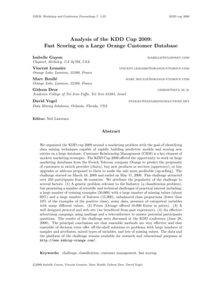
- 5. Analysis of the KDD Cup 2009 train and test sets. A random subset of 10% of the test set was designated to provide immediate performance feed-back. 5. Beta tests The website of the challenge http://www.kddcup-orange.com/ was thoroughly tested by the KDD cup chairs and volunteers. The datasets were downloaded and checked. Baseline methods were tried to verify the feasibility of the task. A Matlab R version of the data was made available and sample code were provided to format the results. A sample submission of random results was given as example and submitted to the website. The results of the Na¨ Bayes method were also uploaded to the website to provide baseline results. ıve Toy problem: The Toy problem on the LARGE dataset consisted of one single predictive continuous variable (V5963) uniformly distributed on the interval [0, 2.0]. The target value was obtained by thresholding V5963 at 1.6 and adding 20% noise. Hence for 80% of the instances, lying in interval [0, 1.6], the fraction of positive examples is 20%; for the remaining 20% lying in interval ]1.6, 2.0], the fraction of positive examples is 80%. The expected value of the AUC (called “true AUC”) can easily be computed1 . Its value is approximately 0.7206. Because of the variance in the sampling process, the AUC effectively computed using the optimal decision rule (called “optimal AUC”) is 0.7196 for the training set and a 0.7230 for the test set. Interestingly, as shown in Figure 1, the optimal solution was outperformed by many participants, up to 0.7263. This illustrates the problem of multiple testing and shows how the best test performance overestimates both the expected value of the AUC and the performance of the optimal decision rule, increasingly with the number of challenge submissions. Basic Na¨ Bayes classifier: ıve The basic Na¨ Bayes classifier (see e.g., Mitchell, 1997) makes simple independence asıve sumptions between features and votes among features with a voting score capturing the correlation of the feature to the target. No feature selection is performed and there are no hyper-parameters to adjust. For the LARGE dataset, the overall score of the basic Na¨ Bayes classifier is 0.6711, ıve with the following results on the test set: • Churn problem : AUC = 0.6468; • Appetency problem : AUC = 0.6453; 1. If we call T the total number of examples, the (expected value of) the total number of examples of the positive class P is the sum of the number of positive examples in the first and the second intervals, i.e., P = (0.2 × 0.8 + 0.8 × 0.2) T = 0.32 T . Similarly, the total number of negative examples is N = (0.8 × 0.8 + 0.2 × 0.2) T = 0.68 T . If we use the optimal decision rule (a threshold on V5963 at 1.6) the number of true positive examples is the sum of the number of true positive examples in the two intervals, i.e., T P = 0 + (0.2 × 0.8) T = 0.16 T . Similarly, the number of true negative examples is T N = (0.8 × 0.8) T = 0.64 T . Hence, the true positive rate is T P R = T P/P = 0.16/0.32 = 0.5 and the true negative rate is T N R = T N/N = 0.64/0.68 0.9412. The balanced accuracy (or the AUC because BAC = AU C in this case) is therefore: BAC = 0.5 (T P R + T N R) = 0.5 (0.5 + 0.9412) = 0.7206. 5
- 6. ´ Guyon, Lemaire, Boulle, Dror, Vogel Test AUC 0.73 Test True Optimal 0.72 0.71 10/3/09 Date 17/3/09 24/3/09 31/3/09 7/4/09 14/4/09 Figure 1: Toy problem test results. • Up-selling problem : AUC=0.7211; As per the rules of the challenge, the participants had to outperform the basic Na¨ ıve Bayes classifier to qualify for prizes. Orange in-house classifier: The Orange in-house classifier is an extension of the Na¨ Bayes classifier, called “Selective ıve Na¨ Bayes classifier” (Boull´, 2007). It includes an optimized preprocessing, variable ıve e selection, and model averaging. It significantly outperforms the basic Na¨ Bayes classifier ıve performance, which was provided to the participants as baseline, and it is computationally efficient: The results were obtained after 3 hours using a standard laptop, considering the three tasks as three different problems. The models were obtained by applying the training process Khiops R only once since the system has no hyper-parameter to adjust. The results of the in-house system were not revealed until the end of the challenge. An implementation of the method is available as shareware from http://www.khiops.com; some participants downloaded it and used it. The requirements placed on the in-house system are to obtain a high classification accuracy, under the following constraints: • Fully automatic: absolutely no hyper-parameter setting, since hundred of models need to be trained each month. • Fast to train: the three challenge marketing problems were trained in less than 3 hours on a mono-processor laptop with 2 Go RAM. • Efficient after deployment: models need to process rapidly up to ten million instances. • Interpretable: selected predictive variables must provide insight. 6
- 7. Analysis of the KDD Cup 2009 However, for the challenge, the participants were not placed under all these constraints for practical reasons: it would have been both too constraining for the participants and too difficult to enforce for the organizers. The challenge focused on maximizing accuracy under time constraints. For the LARGE dataset, the overall score of the Orange in-house classifier is 0.8311, with the following results on the test dataset: • Churn problem : AUC = 0.7435; • Appetency problem : AUC = 0.8522; • Up-selling problem : AUC=0.8975; The challenge was to beat these results, but the minimum requirement to win prizes was only to outperform the basic Na¨ Bayes classifier. ıve 6. Challenge schedule and protocol The key elements of our design were: • To make available the training and test data three weeks before the start of the “fast challenge” to allow participants to download the large volume of data, read it and preprocess it without the training labels. • To make available “toy” training labels during that period so participants could finalize their methodology and practice using the on-line submission system. • To put participants under time pressure once the training labels were released (produce results in five days) to test their ability to produce results in a timely manner. • To continue the challenge beyond this first milestone for another month (slow challenge) to give the opportunity to participants with less computational resources to enter the challenge. • To provide a down-sized version of the dataset for the slow challenge providing an opportunity for participants with yet less computational resources to enter the challenge. • To provide large prizes to encourage participation (10,000 Euros donated by Orange), without any strings attached (no legal constraint or commitment to release code or methods to download data or participate). The competition rules are summarized below are inspired from previous challenges we organized (Clopinet): 1. Conditions of participation: Anybody who complied with the rules of the challenge (KDD cup 2009) was welcome to participate. Only the organizers listed on the Credits page were excluded from participating. The participants were not required to attend the KDD cup 2009 workshop and the workshop was open to anyone. 7
- 8. ´ Guyon, Lemaire, Boulle, Dror, Vogel 2. Anonymity: All entrants had to identify themselves by registering on the KDD cup 2009 website. However, they could elect to remain anonymous during the development period. To be eligible for prizes the had to publicly reveal their identity. Teams had to declare a team leader and register their members. No individual could be part of two or more teams. 3. Data: The datasets were available for download from the Dataset page to registered participants. The data were available in several archives to facilitate downloading. 4. Challenge duration and tracks: The challenge started March 10, 2009 and ended May 11, 2009. There were two challenge tracks: • FAST (large) challenge: Results submitted on the LARGE dataset within five days of the release of the real training labels counted towards the fast challenge. • SLOW challenge: Results on the small dataset and results on the large dataset not qualifying for the fast challenge, submitted before the KDD cup 2009 deadline May 11, 2009, counted toward the SLOW challenge. If more than one submission was made in either track and with either dataset, the last submission before the track deadline was taken into account to determine the ranking of participants and attribute the prizes. 5. On-line feed-back: During the challenge, the training set performances were available on the Result page as well as partial information on test set performances: The test set performances on the “toy problem” and performances on a fixed 10% subset of the test examples for the real tasks (churn, appetency and up-selling). After the challenge was over, the performances on the whole test set were calculated and substituted in the result tables. 6. Submission method: The method of submission was via the form on the Submission page, following a designated format. Results on the “toy problem” did not count as part of the competition. Multiple submissions were allowed, but limited to 5 submissions per day to avoid congestion. For the final entry in the slow track, the participants could submit results on either (or both) small and large datasets in the same archive. 7. Evaluation and ranking: For each entrant, only the last valid entry, as defined in the Instructions counted towards determining the winner in each track (fast and slow). We limited each participating person to a single final entry in each track. Valid entries had to include results on all three real tasks. Prizes could be attributed only to entries performing better than the baseline method (Na¨ Bayes). The results of ıve the baseline method were provided to the participants. 8. Reproducibility: Participation was not conditioned on delivering code nor publishing methods. However, we asked the participants to voluntarily fill out a fact sheet about their methods and contribute papers to the proceedings. 8
- 9. Analysis of the KDD Cup 2009 Figure 2: KDD Cup Participation by year (number of teams). The full rules are available from the website of the challenge http://www.kddcup-orange. com/. The rules were designed to attract a large number of participants and were successful in that respect: Many participants did not participate in the fast challenge on the large dataset, but entered in the slow track, either on the small or the large dataset (or both). There was one minor design mistake: the small dataset was derived from the same data as the large one and, despite our efforts to disguise the identity of the features, it was possible for some entrants to match the features and entries in the small and large dataset. This provided a small advantage, in the slow track only, to the teams who did that data “unscrambling”: they could get feed-back on 20% of the data rather than 10%. The schedule of the challenge was as follows (Dates in 2009): • March 10 - Start of the FAST large challenge. Data tables without target values were made available for the large dataset. Toy training target values were made available for practice purpose. Objective: participants can download data, ask questions, finalize their methodology, try the submission process. • April 6 - Training target values were made available for the large dataset for the real problems (churn, appetency, and upselling). Feed-back: results on 10% of the test set available on-line when submissions are made. • April 10 - Deadline for the FAST large challenge. Submissions had to be received before midnight, time zone of the challenge web server. • April 11 - Data tables and training target values were made available for the small dataset. The challenge continued for the large dataset in the slow track. • May 11 - Deadline for the SLOW challenge (small and large datasets). Submissions had to be be received before midnight, time zone of the challenge web server. 7. Results The 2009 KDD Cup attracted 1299 teams from 46 different countries. From those teams, 7865 valid entries were submitted by 453 different teams. The participation was more than 9
- 10. ´ Guyon, Lemaire, Boulle, Dror, Vogel Prize 1 2 3 1 2 3 Table 1: Winning entries. Country Fast Rank IBM Research USA 1 ID Analytics USA 2 David Slate & Peter Frey USA 3 University of Melbourne Australia 27 Financial Engineering Group, Inc. Japan 4 National Taiwan University Taiwan 20 Team track Score 0.8493 0.8448 0.8443 0.8250 0.8443 0.8332 Slow Rank 1 3 8 2 4 5 track Score 0.8521 0.8479 0.8443 0.8484 0.8477 0.8461 three times greater than any KDD Cup in the past. Figure 2 represents the KDD Cup participation by year. A large participation was a key element to validate the results and for Orange to have a ranking of its in-house system; the challenge was very successful in that respect. 7.1 Winners The overall winner is the IBM Research team (IBM Research, 2009) who ranked first in both tracks. Six prizes were donated by Orange to top ranking participants in the fast and the slow tracks (see Table 1). As per the rules of the challenge, the same team could not earn two prizes. If the ranking of a team entitled it to two prizes, it received the best of the two and the next best ranking team received the other prize. All the winning teams scored best on the large dataset (and most participants obtained better results on the large dataset then on the small dataset). IBM Research, ID Analytics, and National Taiwan University (NTU) “unscrambled” the small dataset. This may have provided an advantage only to NTU since “unscrambling” affected only the slow track and the two other teams won prizes in the fast track. We briefly comment on the results of the winners. Fast track: • IBM Research: The winning entry (IBM Research, 2009) consisted of an ensemble of a wide variety of classifiers, following (Caruana and Niculescu-Mizil, 2004; Caruana et al., 2006). Effort was put into coding (most frequent values coded with binary features, missing values replaced by mean, extra features constructed, etc.) • ID Analytics, Inc.: One of the only teams to use a wrapper feature selection strategy, following a filter (Xie et al., 2009). The classifier was built from the commercial TreeNet software by Salford Systems: an additive boosting decision tree technology. Bagging was also used to gain additional robustness. • David Slate & Peter Frey (Old dogs with new tricks): After a simple preprocessing (consisting in grouping of modalities or discretizing) and filter feature selection, this team used ensembles of decision trees, similar to Random Forests (Breiman, 2001). 10
- 11. Analysis of the KDD Cup 2009 Slow track: • University of Melbourne: This team used for feature selection a cross-validation method targeting the AUC and, for classification, boosting with classification trees and shrinkage, using a Bernoulli loss (Miller et al., 2009). • Financial Engineering Group, Inc.: Few details were released by the team about their methods. They used grouping of modalities and a filter feature selection method using the AIC criterion (Akaike, 1973). Classification was based on gradient treeclassifier boosting (Friedman, 2000). • National Taiwan University: The team averaged the performances of three classifiers (Lo et al., 2009): (1) The solution of the joint multiclass problem with an L1-regularized maximum entropy model. (2) AdaBoost with tree-based weak learners (Freund and Schapire, 1996). (3) Selective Na¨ Bayes (Boull´, 2007), which is ıve e the in-house classifier of Orange (see Section 5). 7.2 Performance statistics We now turn to the statistical analysis of the results of the participants. The main statistics are summarized in Table 2. In the figures of this section, we use the following color code: 1. Black: Submissions received. 2. Blue: Overall best submissions received. Referred to as T estAU C ∗∗ . 3. Red: Baseline result, obtained with the basic Na¨ Bayes classifier or NB, provided ıve by the organizers (see Section 5). The organizers consider that this result is easy to improve. They imposed that the participants would outperform this result to win prizes to avoid that a random submission would win a prize. 4. Green: Orange system result, obtained by the in-house Orange system with the Selective Na¨ Bayes classifier or SNB (see Section 5). ıve Progress in performance Figure 3.a presents the results of the first day. A good result, better than the baseline result, is obtained after one hour and the in-house system is slightly outperformed after seven hours. The improvement during the first day of the competition, after the first 7 hours, is small: from 0.8347 to 0.8385. Figure 3.b presents the results over the first 5 days (FAST challenge). The performance progresses from 0.8385 to 0.8493. The rush of submissions before the deadline is clearly observable. Considering only the submission with Test AUC > 0.5 in the first 5 days, 30% of the submissions had worse results than the baseline (basic Na¨ Bayes) and 91% had worse ıve results than the in-house system (AUC=0.8311). Only and 9% of the submissions had better results than the in-house system. 11
- 12. ´ Guyon, Lemaire, Boulle, Dror, Vogel Table 2: Best results and baselines. The first four lines show the best score T AU C ∗ (averaged over the three tasks), over increasing periods of time [0 : t]. For comparison we give the results of the basic Na¨ Bayes classifier (NB) and the in-house ıve Orange system (SNB). The best overall performance is T AU C ∗∗ = T AU C ∗ (36d). The relative performance difference δ ∗ = (T AU C ∗∗ − T AU C)/T AU C ∗∗ is given in parenthesis (in percentage). The two last lines represent the relative performance difference δ = (T AU C ∗ (t) − T AU C)/T AU C ∗ (t) for the two reference results. T AU C (δ ∗ %) Churn Appetency Up-selling Average δ NB % δ SN B % T AU C ∗ 12h 0.7467 (2.40) 0.8661 (2.17) 0.9011 (0.89) 0.8380 (1.65) 19.92 0.82 T AU C ∗ 24h 0.7467 (2.40) 0.8714 (1.57) 0.9011 (0.89) 0.8385 (1.60) 19.96 0.88 T AU C ∗ 5d 0.7611 (0.52) 0.8830 (0.26) 0.9057 (0.38) 0.8493 (0.33) 20.98 2.14 T AU C ∗∗ 0.7651 (0) 0.8853 (0) 0.9092 (0) 0.8521 (0) 21.24 2.46 T AU C N B 0.6468 (15.46) 0.6453 (27.11) 0.7211 (20.69) 0.6711 (21.24) - T AU C SN B 0.7435 (2.82) 0.8522 (3.74) 0.8975 (1.29) 0.8311 (2.46) - Figures 3.a and 3.b show that good results were obtained already the first day and only small improvements were made later. These results, and an examination of the fact sheets of the challenge filled out by the participants, reveal that: • There are available methods, which can process fast large databases using today’s available hardware in both academia and industry. • Several teams were capable of adapting their methods to meet the requirements of the challenge and reach quickly good performances, yet the bulk of the participants did not. • The protocol of the challenge was well designed: the month given to download the data and play with the submission protocol (using the toy problem) allowed us to monitor progress in performance, not the time required to get ready for the challenge. This last point was important for Orange to assess the time taken for generating stateof-the-art models, since speed of model generation is a key requirement in such applications. The fact that performances do not significantly improve after a few hours is further confirmed in Figure 3.c: very small improvements (from 0.8493 to 0.8521) were made after the 5th day (SLOW challenge)2 . Rapidity of model building Figure 4.d gives a comparison between the submissions received and the best overall result over increasing periods of time: 12 hours, one day, 5 days, and 36 days. We compute the relative performance difference δ ∗ = (T estAU C ∗∗ − T estAU C)/T estAU C ∗∗ , (2) 2. This improvement may be partly attributed to “unscrambling”; unscrambling was not possible during the fast track of the challenge (first 5 days). 12
- 13. Analysis of the KDD Cup 2009 0.8 0.75 0.75 Test AUC 0.85 0.8 Test AUC 0.85 0.7 0.65 0.7 0.65 0.6 0.6 0.55 0.55 0.5 0 1 2 3 4 5 6 7 8 0.5 0 9 10 11 12 13 14 15 16 17 18 19 20 21 22 23 24 24 Hour 48 72 96 120 Hour (a) Test AUC - hour ∈ [0:24] (b) Test AUC - day ∈ [1:5] 0.85 0.8 Test AUC 0.75 0.7 0.65 0.6 0.55 0.5 0 2 4 6 8 10 12 14 16 18 20 22 24 26 28 30 32 34 36 Day (c) Test AUC - day ∈ [0:36] Figure 3: Participant results over time. “Test AUC” is the average AUC on the test set for the three problems. Each point represents an entry. The horizontal bars represent: basic Na¨ Bayes, selective Na¨ Bayes, and best participant entry. ıve ıve where T estAU C ∗∗ is the best overall result. The values of δ ∗ for the best performing classifier in each interval and for the reference results are found in Table 2. The following observations can be made: • there is a wide spread of results; • the median result improves significantly over time, showing that it is worth continuing the challenge to give to participants an opportunity of learning how to solve the problem (the median beats the baseline on all tasks after 5 days but keeps improving); • but the best results do not improve a lot after the first day; 13
- 14. ´ Guyon, Lemaire, Boulle, Dror, Vogel • and the distribution after 5 days is not very different from that after 36 days. Table 2 reveals that, at the end of the challenge, for the average score, the relative performance difference between the baseline model (basic Na¨ Bayes) and the best model ıve is over 20%, but only 2.46% for SNB. For the best ranking classifier, only 0.33% was gained between the fifth day (FAST challenge) and the last day of the challenge (SLOW challenge). After just one day, the best ranking classifier was only 1.60% away from the best result. The in-house system (selective Na¨ Bayes) has a result less than 1% worse than the best ıve model after one day (δ = (1 − 0.8311/0.8385) = 0.88%). We conclude that the participants did very well in building models fast. Building competitive models is one day is definitely doable and the Orange in-house system is competitive, although it was rapidly beaten by the participants. Individual task difficulty To assess the relative difficulty of the three tasks, we plotted the relative performance difference δ ∗ (Equation 2) for increasing periods of time, see Figure4.[a-c]. The churn task seems to be the most difficult one, if we consider that the performance at day one, 0.7467, only increases to 0.7651 by the end of the challenge (see Table 2 for other intermediate results). Figure 4.a shows that the median performance after one day is significantly worse than the baseline (Na¨ Bayes), whereas for the other ıve tasks the median was already beating the baseline after one day. The appetency task is of intermediate difficulty. Its day one performance of 0.8714 increases to 0.8853 by the end of the challenge. Figure 4.b shows that, from day one, the median performance beats the baseline method (which performs relatively poorly on this task). The up-selling task is the easiest one: the day one performance 0.9011, already very high, improves to 0.9092 (less that 1% relative difference). Figure 4.c shows that, by the end of the challenge, the median performance gets close to the best performance. Correlation between T estAU C and V alidAU C: The correlation between the results on the test set (100% of the test set), T estAU C, and the results on the validation set (10% of the test set used to give a feed back to the competitors), V alidAU C, is really good. This correlation (when keeping only AUC test results > 0.5 considering that test AUC < 0.5 are error submissions) is of 0.9960 ± 0.0005 (95% confidence interval) for the first 5 days and of is of 0.9959 ± 0.0003 for the 36 days. These values indicate that (i) the validation set was a good indicator for the online feedback; (ii) the competitors have not overfitted the validation set. The analysis of the correlation indicator task by task gives the same information, on the entire challenge (36 days) the correlation coefficient is for the Churn task: 0.9860 ±0.001; for the Appetency task: 0.9875 ±0.0008 and for the Up-selling task: 0.9974 ±0.0002. Several participants studied the performance estimation variance by splitting the training data multiple times into 90% for training and 10% for validation. The variance in 14
- 15. Analysis of the KDD Cup 2009 80 60 60 Delta* (%) 100 80 Delta* (%) 100 40 20 0 40 20 12h 24h 5d 0 36d 12h (a) Churn 5d 36d (b) Appetency 100 80 80 60 60 Delta* (%) 100 Delta* (%) 24h 40 20 0 40 20 12h 24h 5d 0 36d (c) Up-selling 12h 24h 5d 36d (d) Average Figure 4: Performance improvement over time. Delta∗ represents the relative difference in Test AUC compared to the overall best result T estAU C ∗∗ : Delta∗ = (T estAU C ∗∗ − T estAU C)/T estAU C ∗∗ . On each box, the central mark is the median, the edges of the box are the 25th and 75th percentiles, the whiskers extend to the most extreme data points not considered to be outliers; the outliers are plotted individually as crosses. the results that they obtained led them to use cross-validation to perform model selection rather than relying on the 10% feed-back. Cross-validation was used by all the top ranking participants. This may explain why the participants did not overfit the validation set. We also asked the participants to return training set prediction results, hoping that we could do an analysis of overfitting by comparing training set and test set performances. However, because the training set results did not affect the ranking score, some participants did not return real prediction performances using their classifier, but returned either random results or the target labels. However, if we exclude extreme performances (random or perfect), we can observe that (i) a fraction of the models performing well on test data 15
- 16. ´ Guyon, Lemaire, Boulle, Dror, Vogel have a good correlation between training and test performances; (ii) there is a group of models performing well on test data and having an AUC on training examples significantly larger. Large margin models like SVMs (Boser et al., 1992) or boosting models (Freund and Schapire, 1996) behave in this way. Among the models performing poorly on test data, some clearly overfitted (had a large difference between training and test results). 7.3 Methods employed We analyzed the information provided by the participants in the fact sheets. In Figures 5,6,7, and 8, we show histograms of the algorithms employed for preprocessing, feature selection, classifier, and model selection. We briefly comment on these statistics: • Preprocessing: Few participants did not use any preprocessing. A large fraction of the participants replaced missing values by the mean or the median or a fixed value. Some added an additional feature coding for the presence of a missing value. This allows linear classifiers to automatically compute the missing value by selecting an appropriate weight. Decision tree users did not replace missing values. Rather, they relied on the usage of “surrogate variables”: at each split in a dichotomous tree, if a variable has a missing value, it may be replaced by an alternative “surrogate” variable. Discretization was the second most used preprocessing. Its usefulness for this particular dataset is justified by the non-normality of the distribution of the variables and the existence of extreme values. The simple bining used by the winners of the slow track proved to be efficient. For categorical variables, grouping of under-represented categories proved to be useful to avoid overfitting. The winners of the fast and the slow track used similar strategies consisting in retaining the most populated categories and coarsely grouping the others in an unsupervised way. Simple normalizations were also used (like dividing by the mean). Principal Component Analysis (PCA) was seldom used and reported not to bring performance improvements. • Feature selection: Feature ranking and other filter methods were the most widely used feature selection methods. Most participants reported that wrapper methods overfitted the data. The winners of the slow track method used a simple technique based on cross-validation classification performance of single variables. • Classification algorithm: Ensembles of decision trees were the most widely used classification method in this challenge. They proved to be particularly well adapted to the nature of the problem: large number of examples, mixed variable types, and lots of missing values. The second most widely used method was linear classifiers, and more particularly logistic regression (see e.g., Hastie et al., 2000). Third came non-linear kernel methods (e.g., Support Vector Machines, Boser et al. 1992). They suffered from higher computational requirements, so most participants gave up early on them and rather introduced non-linearities by building extra features. • Model selection: The majority of the participants reported having used to some extent the on-line performance feed-back on 10% of the test set for model selection. However, the winners all declared that they quickly realized that due to variance in the data, this method was unreliable. Cross-validation (ten-fold or five-fold) has been 16
- 17. Analysis of the KDD Cup 2009 PREPROCESSING (overall usage=95%) Replacement of the missing values Discretization Normalizations Grouping modalities Other prepro Principal Component Analysis 0 20 40 Percent of participants 60 80 Figure 5: Preprocessing methods. FEATURE SELECTION (overall usage=85%) Feature ranking Filter method Other FS Forward / backward wrapper Embedded method Wrapper with search 0 10 20 30 40 Percent of participants 50 60 Figure 6: Feature selection methods. the preferred way of selecting hyper-parameters and performing model selection. But model selection was to a large extent circumvented by the use of ensemble methods. Three ensemble methods have been mostly used: boosting (Freund and Schapire, 1996; Friedman, 2000), bagging (Breiman, 1996, 2001), and heterogeneous ensembles built by forward model selection (Caruana and Niculescu-Mizil, 2004; Caruana et al., 2006). Surprisingly, less than 50% of the teams reported using regularization (Vapnik, 1998). Perhaps this is due to the fact that many ensembles of decision trees do not have explicit regularizers, the model averaging performing an implicit regularization. The wide majority of approaches were frequentist (non Bayesian). Little use was made of the unlabeled test examples for training and no performance gain was reported. 17
- 18. ´ Guyon, Lemaire, Boulle, Dror, Vogel CLASSIFIER (overall usage=93%) Decision tree... Linear classifier Non-linear kernel Other Classif - About 30% logistic loss, >15% exp loss, >15% sq loss, ~10% hinge loss. Neural Network Naïve Bayes Nearest neighbors - Less than 50% regularization (20% 2-norm, 10% 1-norm). Bayesian Network - Only 13% unlabeled data. Bayesian Neural Network 0 10 20 30 40 Percent of participants 50 60 Figure 7: Classification algorithms. MODEL SELECTION (overall usage=90%) 10% test K-fold or leave-one-out Out-of-bag est Bootstrap est Other-MS - About 75% ensemble methods (1/3 boosting, 1/3 bagging, 1/3 other). Other cross-valid Virtual leave-one-out - About 10% used unscrambling. Penalty-based Bi-level Bayesian 0 10 20 30 40 Percent of participants 50 60 Figure 8: Model selection methods. We also analyzed the fact sheets with respect to the software and hardware implementation (Figure 9): • Hardware: While some teams used heavy computational apparatus, including multiple processors and lots of memory, the majority (including the winners of the slow track) used only laptops with less than 2 Gbytes of memory, sometimes running in parallel several models on different machines. Hence, even for the large dataset, it was possible to provide competitive solutions with inexpensive computer equipment. In fact, the in-house system of Orange computes its solution in less than three hours on a laptop. 18
- 19. Analysis of the KDD Cup 2009 > 8 GB >= 32 GB Run in parallel <= 8 GB None <= 2GB Multi-processor Memory Parallelism Mac OS Java Other (R, SAS) Matlab Linux Unix Windows C C++ Software Platform Operating System Figure 9: Implementation. • Software: Even though many groups used fast implementations written in C or C++, packages in Java (Weka) and libraries available in Matlab R or “R”, presumably slow and memory inefficient, were also widely used. Users reported performing first feature selection to overcome speed and memory limitations. Windows was the most widely used operating system, closely followed by Linux and other Unix operating systems. 8. Significance Analysis One of the aims of the KDD cup 2009 competition was to find whether there are data-mining methods which are significantly better than others. To this end we performed a significance analysis on the final results (last submission before the deadline, the one counting towards the final ranking and the selection of the prize winners) of both the SLOW and FAST track. Only final results reported on the large dataset were included in the analysis since we have realized that submissions based on the small dataset were considerably inferior. To test whether the differences between the teams are statistically significant we followed a two step analysis that is specifically designed for multiple hypothesis testing when several independent task are involved (Demˇar, 2006): First we used the Friedman test (Friedman, s 1937), to examine the null hypothesis H0 , which states that the AUC values of the three tasks, (Churn, Appetency and Up-Selling) on a specific track (FAST or SLOW) are all drawn from a single distribution. The Friedman test is a non-parametric test, based on the average ranking of each team, where AUC values are ranked for each task separately. A simple test-statistic of the average ranks is sufficient to extract a p-value for H0 ; In the case when H0 is rejected, we use a two tailed Nemenyi test (Nemenyi, 1963) as a post-hoc analysis for identifying teams with significantly better or worse performances. Not surprisingly, if one takes all final submissions, one finds that H0 is rejected with high certainty (p-value < 10−12 ). Indeed, significant differences are observed even when one inspects the average final AUCs (see Figure 10), as some submissions were not substantially 19
- 20. ´ Guyon, Lemaire, Boulle, Dror, Vogel (a) FAST (b) SLOW Figure 10: Sorted final scores: The sorted AUC values on the test set of each of the three tasks, together with the average of AUC on the three tasks. Only final submissions are included. (a) FAST track and (b) SLOW track. The baselines for the basic Na¨ Bayes and selective Na¨ Bayes are superposed on the ıve ıve corresponding tasks. better than random guess, with an AUC near 0.5. Of course, Figure 10 is much less informative than the significance testing procedure we adopt, which combines the precise scores on the three tasks, and not each one separately or their averages. Trying to discriminate among the top performing teams is more subtle. When taking the best 20 submissions per track (ranked by the best average AUC) - the Friedman test still rejects H0 with p-values 0.015 and 0.001 for the FAST and SLOW tracks respectively. However, the Nemenyi tests on these reduced data are not able to identify significant differences between submissions, even with a significance level of α = 0.1! The fact that one does not see significant differences among the top performing submissions is not so surprising: during the period of the competition more and more teams have succeeded to cross the baseline, and the best submissions tended to accumulate in the tail of the distribution (bounded by the optimum) with no significant differences. This explains why the number of significant differences between the top 20 results decreases with time and number of submissions. Even on a task by task basis, Figure 10 reveals that the performance of the top 50% AUC values lie on an almost horizontal line, indicating there are no significant differences among these submissions. This is especially marked for the SLOW track. From an industrial point of view, this result is quite interesting. In an industrial setting many criteria have to be considered (performance, automation of the data mining process, training time, deployment time, etc.). But this significance testing shows using state-of the art techniques, one is unlikely to get significant improvement of performance even at the expense of a huge deterioration of the other criterions. 20
- 21. Analysis of the KDD Cup 2009 9. Conclusion The results of the KDD cup 2009 exceeded our expectations in several ways. First we reached a very high level of participation: over three times as much as the most popular KDD cups so far. Second, the participants turned in good results very quickly: within 7 hours of the start of the FAST track challenge. The performances were only marginally improved in the rest of the challenge, showing the maturity of data mining techniques. Ensemble of decision trees offer off-the-shelf solutions to problems with large numbers of samples and attributes, mixed types of variables, and lots of missing values. Ensemble methods proved to be effective for winning, but single models are still preferred by many customers. Further work include matching the performances of the top ranking participants with single classifiers. Acknowledgments We are very grateful to the Orange company who donated the data, the computer servers, many hours of engineer time, and the challenge prizes. We would like to thank all the Orange team members, including Fabrice Cl´rot and Raphael F´raud. We also gratefully e e acknowledge the ACM SIGKDD and the Pascal2 European network of excellence (FP7-ICT2007-1-216886) who supported the work of the KDD Cup 2009 co-chairs Isabelle Guyon and David Vogel and the web site development. The support of Google and Health Discovery Corporation allowed students to attend the workshop. We are very grateful to the technical support of MisterP and Pascal Gouzien. We also thank Gideon Dror for editing the proceedings. References H. Akaike. Information theory and an extension of the maximum likelihood principle. In B.N. Petrov and F. Csaki, editors, 2nd International Symposium on Information Theory, pages 267–281. Akademia Kiado, Budapest, 1973. Bernhard E. Boser, Isabelle Guyon, and Vladimir Vapnik. A training algorithm for optimal margin classifiers. In COLT, pages 144–152, 1992. Marc Boull´. Compression-based averaging of Selective Na¨ Bayes classifiers. JMLR, 8: e ıve 1659–1685, 2007. ISSN 1533-7928. Leo Breiman. Bagging predictors. Machine Learning, 24(2):123–140, 1996. Leo Breiman. Random forests. Machine Learning, 45(1):5–32, 2001. Rich Caruana, Art Munson, and Alexandru Niculescu-Mizil. Getting the most out of ensemble selection. In Proceedings of the 6th International Conference on Data Mining (ICDM ‘06), December 2006. Full-length version available as Cornell Technical Report 2006-2045. 21
- 22. ´ Guyon, Lemaire, Boulle, Dror, Vogel Rich Caruana and Alexandru Niculescu-Mizil. Ensemble selection from libraries of models. In Proceedings of the 21st International Conference on Machine Learning (ICML’04), 2004. ISBN 1-58113-838-5. Clopinet. Challenges in machine learning. URL http://clopinet.cm/challenges. Janez Demˇar. Statistical comparisons of classifiers over multiple data sets. J. Mach. Learn. s Res., 7:1–30, 2006. ISSN 1533-7928. Yoav Freund and Robert E. Schapire. Experiments with a new boosting algorithm. In ICML, pages 148–156, 1996. Jerome H. Friedman. Greedy function approximation: A gradient boosting machine. Annals of Statistics, 29:1189–1232, 2000. M. Friedman. The use of ranks to avoid the assumption of normality implicit in the analysis of variance. Journal of the American Statistical Association, 32:675–701, 1937. I. Guyon, A. Saffari, G. Dror, and J. Buhmann. Performance prediction challenge. In IEEE/INNS conference IJCNN 2006, Vancouver, Canada, July 16-21 2006. T. Hastie, R. Tibshirani, and J. Friedman. The Elements of Statistical Learning, Data Mining, Inference and Prediction. Springer Verlag, 2000. IBM Research. Winning the KDD cup orange challenge with ensemble selection. In JMLR W&CP, volume 7, KDD cup 2009, Paris, 2009. Hung-Yi Lo et al. An ensemble of three classifiers for KDD cup 2009: Expanded linear model, heterogeneous boosting, and selective na¨ Bayes. In JMLR W&CP, volume 7, ıve KDD cup 2009, Paris, 2009. Hugh Miller et al. Predicting customer behaviour: The University of Melbourne’s KDD cup report. In JMLR W&CP, volume 7, KDD cup 2009, Paris, 2009. T.M. Mitchell. Machine Learning. McGraw-Hill Co., Inc., New York, 1997. P. B. Nemenyi. Distribution-free multiple comparisons. Doctoral dissertation, Princeton University, 1963. V. Vapnik. Statistical Learning Theory. John Wiley and Sons, N.Y., 1998. Jainjun Xie et al. A combination of boosting and bagging for KDD cup 2009 - fast scoring on a large database. In JMLR W&CP, volume 7, KDD cup 2009, Paris, 2009. 22