This research investigates the use of convolutional neural networks and YOLOv5 for detecting license plates in photographs taken by speed cameras in Lima, Peru, utilizing a dataset of 2,000 images. The study optimized training through stochastic gradient descent (SGD) and Adam methods, concluding that SGD achieved better loss function convergence and accuracy metrics. The findings suggest that SGD outperforms Adam, especially in applications involving deep learning for object detection.

1. Convolutional neural networks and YOLOv5 for the
detection of license plates in digital photographic
images
Guillermo Enrique Medina Zegarra
Graduate School
Department of Systems and Informatics Engineering
Universidad Nacional Mayor de San Marcos
Lima, Peru
guillermoemz@gmail.com
Ciro Rodriguez Rodriguez
School of System Engineering and Informatic
Universidad Nacional Mayor de San Marcos
Lima, Peru
crodriguezro@unmsm.edu.pe
Edgar Lobaton
School of Electrical and Computer Engineering
North Caroline State University
North Caroline, USA
ejlobato@ncsu.edu
Roger Chipa Sierra
School of Economic Engineering and Statistics
Universidad Nacional de Ingenierı́as
Lima, Peru
rogerchipa@gmail.com
Abstract—In this research, a dataset of two thousand images
was obtained, which were taken through a speed camera to
vehicles in the city of Lima, Peru, with the purpose of detecting
license plates. Therefore, a distribution of this dataset was
made: 70% for training (1400 images), 20% for validation
(400 images), and 10% for testing (200 images). To visualize
and analyze the behavior and convergence of the loss function,
a distribution was made using the cross-validation method
with the following three folds: 1400, 840, and 280, with
two optimization methods (stochastic gradient descent with
momentum and Adam), both optimization techniques were used
for training from scratch and transfer learning. The results
obtained demonstrated that the loss function converges better
with the first optimization method. We used precision metric, too.
Keywords: Convolutional neuronal network, deep learning,
YOLO, SGD, Adam.
I. INTRODUCTION
In Peru, due to infrastructure and logistics limitations, there
were problems in the production and distribution of vehicle
license plates throughout the country. As a consequence, there
was chaos and informality in the circulation of different
vehicles nationwide, with counterfeit license plates being used.
Another identified deficiency was the lack of standardization
of vehicle license plates. As a result, the Peruvian government
approved a law [1] to standardize and uniformize the license
plates of different vehicles; in a world increasingly globalized
and with technological advancements, new technological alter-
natives and deep learning methods have emerged to automate
object detection.
Therefore, recent advancements in deep learning [2], [3],
[4], [5], [6], [7] [8] have contributed to various fields of
artificial intelligence, such as: natural language processing,
reinforcement learning, board games, card games and com-
puter vision. The use of deep convolutional neural networks [9]
[10] [11] [12] has enabled vehicle license plate and character
detection and recognition [13], weapon detection [14], facial
expression recognition [15], improvement in translations, and
more. Therefore, it is crucial to determine which optimization
method [16], [17], [18] [19] best converges the learning model
during the training and validation of deep neural networks.
II. THEORETICAL FRAMEWORK
A. Machine learning
Machine learning [20] is a branch of Artificial Intelligence
that aims to develop computational algorithms [21] [22] so
that computers can learn from a dataset, thereby creating
a predictive model. In the case of predictive or supervised
machine learning, projections can be created based on data.
On the other hand, with descriptive or unsupervised machine
learning, it does not allow making predictions but instead
recognizes patterns [23]. Through these patterns, it can detect
and classify objects using images autonomously, grouping data
based on similar or common features. Finally, the third and
last type of machine learning classification is reinforcement
learning [24], which involves learning through “reward” or
“punishment” from an environment. Thus, machine learning
is categorized into supervised learning, unsupervised learning,
and reinforcement learning.
A fundamental difference between deep learning and tradi-
tional machine learning is that deep learning exclusively uses
deep neural networks [25] to automatically solve the regres-
sion and classification problem of objects, unlike traditional
machine learning, which performs part of the process manually

2. or semi-manually and the other part automatically using a
classification method. For a better illustration, see Figure 1.
Fig. 1: Tradicional machine learning vs. deep learnig [26].
B. Convolutional Neuronal Network (CNN)
David Hubel y Torsten Wiesel [27], both from the Harvard
Medical School, conducted a series of studies and experiments
on the visual cortex of cats in the 1950s. They concluded that
many neurons in the visual cortex have a small local receptive
field through which they respond to visual stimuli located in
a specific region of the visual field. The receptive fields of
different neurons can overlap and join to form a complete
visual field. On the other hand, the authors demonstrated that
some neurons only respond to different orientations, such as a
line (see Figure 2a). They also observed that other neurons
have larger receptive fields and respond to more complex
patterns, which are combinations of lower-level patterns [20].
(a) Receptive field of a cat’s visual cortex [27].
(b) Illustration of a deep learning model, with an input layer,
three hidden layers, and an output layer [28].
(c) Convolutional Neural Network Architecture [29].
Fig. 2: Visual cortex of cats, deep learning model and CNN
architecture.
Then visual cortex of cats inspired the Neocognitron [30],
which was a model of a neural network for visual pattern
recognition. Years later, Yann LeCunn, León Bottou, Yoshua
Bengio, and Patrick Haffner designed a new model of neural
network, which allowed the use of multiple layers enabling
a process of feed-forward and backpropagation [25], solving
the classification and regression problem of object detection
(see subfigure 2c). They called the first architecture of con-
volutional neural networks LeNet-5 [31], and consequently, a
new type of artificial neural network emerged. Several years
later, Geoffrey Hinton, Ian Goodfellow, Yoshua Bengio, Aaron
Courville, among other researchers, would give more formality
to this new area called deep learning [28]. In Figure 2b,
you can see an illustration of a deep learning model can be
observed, starting with the input layer (visible layer), through
which the input variables (pixels) are fed; then, three hidden
layers can be seen, one for edge detection, another for corner
and contour detection, and the third hidden layer for the
creation or combination of object parts; after the hidden layers,
there is an output layer, through which the identification of a
classified object is obtained, such as a car, person, or animal.
The architectures of convolutional neural networks are
mainly composed of: convolutional layers, pooling layers, and
fully-connected layers.
C. Object detection
In Figure 3, the evolution of different techniques in object
detection can be observed. Starting with traditional methods,
which began with the SIFT (Scale-Invariant Feature Trans-
form) algorithm [32] [33], published in 1999. It analyzes
the image at different scales and with different levels of
smoothing (DoG), considering maximum and minimum values
and discarding irrelevant points. It is invariant to rotation,
scaling, translation, changes in illumination, and perspective.
Next, in 2001, the technique of cascading classification, also
known as Haar Cascades [34] [35], appeared. It uses Haar
features to detect patterns in an image, creating sliding win-
dows and working with features rather than pixels. The con-
catenation or combination of these advantages allows creating
strong classifiers with the support of AdaBoost. In 2005,
the HOG (Histogram of Oriented Gradients) method [36]
emerged, which allows feature extraction by concatenating
all the normalized histograms from dividing the image into
small squares, creating a feature vector, which can be useful
as input data for classification through Support Vector Machine
(SVM). In 2006, the SURF (Speeded-Up Robust Features)
technique [37] appeared as an improved version of the SIFT
method, being faster and robust to transformations. It uses
the Hessian Beaudet detector [38] to detect edges, replacing
DoG. Similarly, it uses signal processing through Haar Wavelet
[39] to represent features or interest points. In 2008, the DPM
(Deformable Part-based Models) technique [40] extended the
HOG detector, using the principle of divide and conquer
[41]. It divides the object into parts and models the spatial
relationships between them. By dividing the object into parts,
it provides input data to be used with a classifier like Support

3. Fig. 3: Evolution of object detection techniques [4] [5].
Vector Machine to identify part of the object. Finally, in
2011, a method called ”Selective Search” [42] emerged to
identify regions of interest (bounding boxes) through ex-
haustive search and segmentation. In 2012, PhD. Geoffrey
Hinton, together with Alex Krizhevsky and Ilya Sutskever,
created a convolutional neural network [11] called AlexNet
[43], which won the ImageNet Large Scale Visual Recognition
Challenge (ILSVRC) [44] of that year. They demonstrated that
feature learning (feature engineering) provides better results
than those designed or obtained manually. Consequently, from
2012, there was a surge in convolutional neural networks
and the beginning of object detection methods based on deep
learning [4] [3], as shown in Figure 3. From that year onwards,
a bifurcation can be observed, where the first division is based
on region-based methods [2] or two-stage frameworks [4] [3]
[5], whose methods include: R-CNN [45], Spatial Pyramid
Pooling (SPP-Net) [46], Fast R-CNN [47], Faster R-CNN
[48], Region Fully Convolutional Networks (R-FCN) [49],
Feature Pyramid Network (FPN) [50], and Mask R-CNN [51].
The second division is based on classification and regression
or one-stage frameworks, whose techniques include: YOLO
[52], Single Shot Multibox Detection (SSD) [53], Retina-Net
[54], CornerNet [55], CenterNet [56], and DETR (DEtection
TRansformer) [57].
Fig. 4: Components of a modern object detector [58].
On the other hand, in Figure 4, the components of a
modern object detector [58] can be observed, such as the
backbone, neck, and head, which are used to predict classes
and bounding boxes of objects. Additionally, it can be seen
that there are two types of heads, one for dense prediction
(single-stage detectors) and another for sparse prediction (two-
stage detectors), both responsible for predicting classes and
bounding boxes. The backbone consists of pre-trained models
for image classification, and the learned and extracted features
are subsequently useful for object detection (regression). The
neck comprises layers after the backbone that are useful for
fusing or combining features from different scales.
D. YOLO
In subfigure 5a, the first five versions of the YOLO family
can be observed. Similarly, for each YOLO version, different
defined architectures exist, where some of the fundamental
differences among them include the number of convolutional
layers, the number of neurons in the hidden layers, and the
different sizes of input images. For instance, YOLOv2 [59]
uses the architecture of the convolutional neural network called
darknet-19 [60], while YOLOv3 [61] utilizes the architecture
of the convolutional neural network known as darknet-53,
which is an improved version with the inclusion of residual
connections. Both YOLOv4 [58] and YOLOv5 [62] use CSP-
Darknet53 as their backbone, and the development of YOLOv5
was done through PyTorch, in contrast to previous versions
that used Darknet. For a better understanding, please refer to
Table I. On the other hand, in subfigure 5b, a benchmark of the
following five YOLOv5 architectures can be seen: YOLOv5n
(nano), YOLOv5s (small), YOLOv5m (medium), YOLOv5l
(large), and YOLOv5x (extra-large). These models, also called
P5 models, have been designed to work with images of 640 x
640 resolution.

4. (a) Versions of YOLO. (b) Benchmark of YOLOv5.
Fig. 5: Versions and benchmark YOLOv5 [63] [64] [62].
TABLE I: Versions of YOLO with their respective backbone
and size [8].
Versión YOLO Backbone Tamaño
YOLOv1 VGG16 448x448
YOLOv2 Darknet19 544x544
YOLOv3 Darknet53 608x608
YOLOv4 CSP-Darknet53 608x608
YOLOv5 CSP-Darknet53 640x640
III. DEVELOPMENT OF THE PROPOSAL
A. Description of hardware, operating system and software
We used Google CodeLabs for training and validation tests,
with the following technical characteristics:
• Ubuntu 20.04.6 LTS x86 64
• Kernel 5.15.107+
• Bash 5.0.17
• CPU: Intel Xeon (2) @ 2.199GHz
• Memory: 1310MiB / 12982MiB
• Python-3.10.12
• Torch-2.0.1+cu118
B. Data collection technique
On the Figure 6, you can see two perspectives of one
Kustom Signal cinemometer equipment, LaserCam4 model,
through this equipment all the images were taken with a size
of 720x576, 72 ppp and 24 bits.
(a) Frontal view (b) Lateral view
Fig. 6: Kustom Signal cinemometer equipment, LaserCam4
model [65].
C. Dataset size
The size of the dataset or total set of images was of two
thousand (2000), these quantity of images were useful for the
evaluation of the model through the k-fold cross-validation
method [20] for three folds of a similar proportion to 560
images, then, the numerical number of images in the training
stage were the following: 1400, 840 and 280; on the other
hand, the numerical quantity of images, in the validation and
testing phase, were 400 and 200 respectively, the quantities are
the same in the three divisions, as detailed in the following
three Tables:
TABLE II: First fold of the dataset of images.
Percentage Numeric quantity Dataset
70% 1,400 Training
20% 400 Validation
10% 200 Testing
TABLE III: Second fold of the dataset of images.
Percentage Numeric quantity Dataset
42% 840 Training
20% 400 Validation
10% 200 Testing
TABLE IV: Third fold of the dataset of images.
Percentage Numeric quantity Dataset
14% 280 Training
20% 400 Validation
10% 200 Testing
D. Optimization
On the Tabla V, you can watch the two optimization
methods used for the three folds for a similar proportion to
560 images described on Tables II, III y IV of the previous
section, these three divisions have as a dataset: training with
a batch-size of 64, the object is to create the best model.
TABLE V: Optimization methods used for each training.
Numeric quantity Dataset Optimization
1,400 Training SGD Adam
840 Training SGD Adam
280 Training SGD Adam
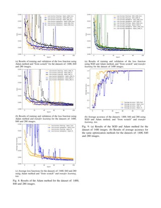
IV. RESULTS
On the subfigures 7a 7b 8a and 8b you can see four images
with the results obtained using the optimization methods SGD
and Adam, for from scratch and transfer learning training, for
the three proposed datasets of: 1400, 840 and 280 images.
On the subfigures 7c, 8c and 9b, the averages of the three
proposed datasets are shown. The subfigure 9a presents a
comparative image of the loss function for the dataset of

5. 1400 images, comparing both optimization techniques and
types of training.
Comparison of the metric accuracy for the two kind of
optimization methods SGD and Adam, and results for each
type of training (from scratch and transfer learning) for the
dataset of 1400 images.
TABLE VI: Results of the metric accuracy for both kind of
optimization SGD and ADAM and for both kind of training.
Accuracy
From scratch Transfer learning
SGD Adam SGD Adam
Average 0.941809066 0.905593933 0.9754841 0.895573062
Standard
deviation
0.2150393 0.272966644 0.113164982 0.269715075
# epoch 100 100 100 100
A. Analysis of results
Now, a demonstration of the general hypothesis, for the case
of the precision metric, with the results obtained on Table VI.
TABLE VII: Proof of the general hypothesis for the precision
metric.
General hypothesis SGD optimization method has better results than Adam,
regarding the precision metric.
Specific hypothesis 1 SGD is better, in terms of accuracy metric, than Adam from
scratch.
Specific hypothesis 2 SGD is better, in terms of accuracy metric, than Adam with
transfer learning.
Test of Specific Hypothesis 1
• Final specific hypothesis: SGD is better, in terms of
accuracy metric, than Adam from scratch.
Null hypothesis:
H0 : µSGD ≥ µAdam (1)
Alternative hypothesis:
H1 : µSGD < µAdam (2)
• Significance level α = 0.05
• Z-test for the difference of means of the specific hypoth-
esis 1
Z =
(X̄1 − X̄2) − ∆
q
σ2
1
n1
+
σ2
2
n2
(3)
Where:
x̄1 : Average of the first sample (method)
x̄2 : Average of the second sample (method)
∆ : Difference of means for null hypothesis
σ2
1 : Standard deviation of the first sample
σ2
2 : Standard deviation of the second sample
n1 : Size of the first sample
n2 : Size of the second sample
Z1 = 1.04217 (4)
• After calculating the value Z1, locate it in the Table of
Standard Normal Distribution [66] and test the null hy-
pothesis of the final specific hypothesis H0 (see equation
1) of the final specific hypothesis 1 and obtain a positive
result, H0 is accepted.
For the case of the test of specific hypothesis 2, the same
procedure is performed, where in this case it would be Z2
and its result would be: Z2 = 2.73206. Now, after calculating
the value Z2 and locating it in the Table of Standard Normal
Distribution, and testing the null hypothesis of its final specific
hypothesis H0, a positive result is obtained, therefore H0 is
also accepted.
V. CONCLUSION
• More quantity of images inside of the dataset (1400, 840
y 280), it will be converge of loss function is better; as
well as the results of metric accuracy.
• YOLOv5 is a detection method, based on deep learning,
it has proven to be a good method for detecting vehicle
license plates; for this reason, to use supervised learning
with deep convolutional neural networks is useful.
• How specific hypothesis 1 and 2 have been acepted,
then it can concluded that the stochastic gradient descent
optimization method is better than Adam, for the type of
training of transfer learning versus training from scratch
with the dataset of 1400 images.
• To use detection methods based on deep learning is good,
because it has advantage such as transfer learning. It can
reduce time of training for have models pre-trained.
LIMITATIONS AND FUTURE WORK
The most important limitation found was the technological
resource (hardware) for the training of the three proposed
datasets, either for the type of training from scratch or transfer
learning. As future work, it would be good to obtain better
hardware resources, to evaluate excellent detection methods
with deep learning, such as the transformers [57].
ACKNOWLEDGMENT
A special thanks to the National Police of Peru and National
University of San Marcos for education.
REFERENCES
[1] MTC, Decreto Supremo que aprueba el reglamento del Sistema de
Placa Única Nacional de Rodaje - Exposición de motivos. Ministerio
de Transporte y Comunicaciones - Dirección General de Transporte
Terrestre.
[2] Z. Zhao, P. Zheng, S. Xu, and X. Wu, “Object detection with
deep learning: A review,” CoRR, vol. abs/1807.05511, 2018. [Online].
Available: http://arxiv.org/abs/1807.05511
[3] Z. Zou, K. Chen, Z. Shi, Y. Guo, and J. Ye, “Object detection in 20
years: A survey,” 2023.
[4] Z. Zou, Z. Shi, Y. Guo, and J. Ye, “Object detection in 20 years:
A survey,” CoRR, vol. abs/1905.05055, 2019. [Online]. Available:
http://arxiv.org/abs/1905.05055

6. [5] L. Liu, W. Ouyang, X. Wang, P. W. Fieguth, J. Chen, X. Liu,
and M. Pietikäinen, “Deep learning for generic object detection:
A survey,” CoRR, vol. abs/1809.02165, 2018. [Online]. Available:
http://arxiv.org/abs/1809.02165
[6] L. Jiao, F. Zhang, F. Liu, S. Yang, L. Li, Z. Feng, and R. Qu, “A survey
of deep learning-based object detection,” CoRR, vol. abs/1907.09408,
2019. [Online]. Available: http://arxiv.org/abs/1907.09408
[7] S. S. A. Zaidi, M. S. Ansari, A. Aslam, N. Kanwal, M. N.
Asghar, and B. Lee, “A survey of modern deep learning based
object detection models,” CoRR, vol. abs/2104.11892, 2021. [Online].
Available: https://arxiv.org/abs/2104.11892
[8] J. Deng, X. Xuan, W. Wang, Z. Li, H. Yao, and Z. Wang, “A review of
research on object detection based on deep learning,” Journal of Physics:
Conference Series, vol. 1684, no. 1, p. 012028, nov 2020. [Online].
Available: https://dx.doi.org/10.1088/1742-6596/1684/1/012028
[9] M. D. Zeiler and R. Fergus, “Visualizing and understanding convolu-
tional networks.” CoRR, vol. abs/1311.2901, 2013. [Online]. Available:
http://dblp.uni-trier.de/db/journals/corr/corr1311.html#ZeilerF13
[10] K. Simonyan and A. Zisserman, “Very deep convolutional networks
for large-scale image recognition,” 2015. [Online]. Available: https:
//arxiv.org/abs/1409.1556
[11] S. Khan, H. Rahmani, S. A. A. Shah, and M. Bennamoun, “A guide to
convolutional neural networks for computer vision,” Synthesis Lectures
on Computer Vision, vol. 8, no. 1, pp. 1–207, 2018. [Online]. Available:
https://doi.org/10.2200/S00822ED1V01Y201712COV015
[12] C. Aggarwal, Neural Networks and Deep Learning: A Textbook.
Springer International Publishing, 2018. [Online]. Available: https:
//books.google.com.pe/books?id=achqDwAAQBAJ
[13] S. M. Silva and C. R. Jung, “A flexible approach for automatic license
plate recognition in unconstrained scenarios,” IEEE Transactions on
Intelligent Transportation Systems, vol. 23, no. 6, pp. 5693–5703, 2022.
[14] S. Narejo, B. Pandey, D. Esenarro Vargas, C. Rodriguez, and M. An-
jum, “Weapon detection using yolo v3 for smart surveillance system,”
Mathematical Problems in Engineering, vol. 2021, pp. 1–9, 05 2021.
[15] J. Bustamante, C. Rodriguez, and D. Esenarro, “Real time facial expres-
sion recognition system based on deep learning,” International Journal
of Recent Technology and Engineering, vol. 8, Issue-2S11), pp. 4047–
4051, 09 2019.
[16] D. P. Kingma and J. Ba, “Adam: A method for stochastic optimization,”
in ICLR (Poster), 2015.
[17] S. Ruder, “An overview of gradient descent optimization algorithms,”
CoRR, vol. abs/1609.04747, 2016. [Online]. Available: http://arxiv.org/
abs/1609.04747
[18] I. Sutskever, J. Martens, G. Dahl, and G. Hinton, “On the
importance of initialization and momentum in deep learning,” in
Proceedings of the 30th International Conference on Machine
Learning, ser. Proceedings of Machine Learning Research, S. Dasgupta
and D. McAllester, Eds., vol. 28, no. 3. Atlanta, Georgia,
USA: PMLR, 17–19 Jun 2013, pp. 1139–1147. [Online]. Available:
https://proceedings.mlr.press/v28/sutskever13.html
[19] J. Moré, “The levenberg-marquardt algorithm: Implementation and
theory,” in Numerical Analysis, ser. Lecture Notes in Mathematics,
G. Watson, Ed., 1978, vol. 630, pp. 105–116.
[20] A. Géron, Hands-on Machine Learning with Scikit-Learn, Keras, and
TensorFlow: Concepts, Tools, and Techniques to Build Intelligent
Systems. O’Reilly Media, Incorporated, 2019. [Online]. Available:
https://books.google.com.pe/books?id=OCS1twEACAAJ
[21] S. Russell, P. Norvig, and J. Rodrı́guez, Inteligencia artificial:
un enfoque moderno, ser. Colección de Inteligencia Artificial
de Prentice Hall. Pearson Educación, 2004. [Online]. Available:
https://books.google.com.pe/books?id=yZCVPwAACAAJ
[22] S. Russell and P. Norvig, Artificial Intelligence: A Modern Approach,
3rd ed. Prentice Hall, 2010.
[23] S. Theodoridis and K. Koutroumbas, Pattern Recognition, Fourth Edi-
tion. Academic Press, 2009.
[24] R. S. Sutton and A. G. Barto, Reinforcement Learning: An
Introduction, 2nd ed. The MIT Press, 2018. [Online]. Available:
http://incompleteideas.net/book/the-book-2nd.html
[25] D. E. Rumelhart, G. E. Hinton, and R. J. Williams, “Learning in-
ternal representations by error propagation,” in Parallel Distributed
Processing: Explorations in the Microstructure of Cognition, Volume 1:
Foundations, D. E. Rumelhart and J. L. Mcclelland, Eds. Cambridge,
MA: MIT Press, 1986, pp. 318–362.
[26] S. Dey., CNN application on structured data-Automated Feature Extrac-
tion. Towards Data Science.
[27] D. H. Hubel and T. N. Wiesel, “Receptive fields and functional archi-
tecture of monkey striate cortex,” Journal of Physiology (London), vol.
195, pp. 215–243, 1968.
[28] I. Goodfellow, Y. Bengio, and A. Courville, Deep Learning. MIT Press,
2016, http://www.deeplearningbook.org.
[29] S. Saha., A Comprehensive Guide to Convolutional Neural Networks.
Towards Data Science.
[30] K. Fukushima, “Neocognitron: A self-organizing neural network model
for a mechanism of pattern recognition unaffected by shift in position,”
Biological Cybernetics, vol. 36, pp. 193–202, 1980.
[31] Y. Lecun, L. Bottou, Y. Bengio, and P. Haffner, “Gradient-based learning
applied to document recognition,” Proceedings of the IEEE, vol. 86,
no. 11, pp. 2278–2324, 1998.
[32] D. Lowe, “Object recognition from local scale-invariant features,” in
Proceedings of the Seventh IEEE International Conference on Computer
Vision, vol. 2, 1999, pp. 1150–1157 vol.2.
[33] D. G. Lowe, “Distinctive image features from scale-invariant keypoints,”
International Journal of Computer Vision, vol. 60, pp. 91–110, 2004.
[34] P. Viola and M. Jones, “Rapid object detection using a boosted cascade
of simple features,” in Proceedings of the 2001 IEEE Computer Society
Conference on Computer Vision and Pattern Recognition. CVPR 2001,
vol. 1, 2001, pp. I–I.
[35] ——, “Robust real-time face detection,” in Proceedings Eighth IEEE
International Conference on Computer Vision. ICCV 2001, vol. 2, 2001,
pp. 747–747.
[36] N. Dalal and B. Triggs, “Histograms of oriented gradients for human
detection,” in 2005 IEEE Computer Society Conference on Computer
Vision and Pattern Recognition (CVPR’05), vol. 1, 2005, pp. 886–893
vol. 1.
[37] H. Bay, T. Tuytelaars, and L. Van Gool, “Surf: Speeded up robust
features.” vol. 110, 01 2006, pp. 404–417.
[38] P. Beaudet, “Rotationally invariant image operators,” 1978.
[39] C. Harris and M. Stephens, “A combined corner and edge detector,” in
In Proc. of Fourth Alvey Vision Conference, 1988, pp. 147–151.
[40] P. Felzenszwalb, D. McAllester, and D. Ramanan, “A discriminatively
trained, multiscale, deformable part model,” in 2008 IEEE Conference
on Computer Vision and Pattern Recognition, 2008, pp. 1–8.
[41] T. Cormen, C. Leiserson, R. Rivest, and C. Stein, Introduction to Algo-
rithms, third edition, ser. The MIT Press. MIT Press, 2009. [Online].
Available: https://books.google.com.pe/books?id=F3anBQAAQBAJ
[42] J. Uijlings, K. Sande, T. Gevers, and A. Smeulders, “Selective search
for object recognition,” International Journal of Computer Vision, vol.
104, pp. 154–171, 09 2013.
[43] A. Krizhevsky, I. Sutskever, and G. E. Hinton, “Imagenet classification
with deep convolutional neural networks,” in Advances in Neural
Information Processing Systems 25, F. Pereira, C. J. C. Burges,
L. Bottou, and K. Q. Weinberger, Eds. Curran Associates, Inc.,
2012, pp. 1097–1105. [Online]. Available: http://papers.nips.cc/paper/
4824-imagenet-classification-with-deep-convolutional-neural-networks.
pdf
[44] O. Russakovsky, J. Deng, H. Su, J. Krause, S. Satheesh, S. Ma,
Z. Huang, A. Karpathy, A. Khosla, M. Bernstein, A. C. Berg, and
L. Fei-Fei, “ImageNet Large Scale Visual Recognition Challenge,”
International Journal of Computer Vision (IJCV), vol. 115, no. 3, pp.
211–252, 2015.
[45] R. B. Girshick, J. Donahue, T. Darrell, and J. Malik, “Rich
feature hierarchies for accurate object detection and semantic
segmentation,” CoRR, vol. abs/1311.2524, 2013. [Online]. Available:
http://arxiv.org/abs/1311.2524
[46] K. He, X. Zhang, S. Ren, and J. Sun, “Spatial pyramid pooling
in deep convolutional networks for visual recognition,” CoRR, vol.
abs/1406.4729, 2014. [Online]. Available: http://arxiv.org/abs/1406.4729
[47] R. B. Girshick, “Fast R-CNN,” CoRR, vol. abs/1504.08083, 2015.
[Online]. Available: http://arxiv.org/abs/1504.08083
[48] S. Ren, K. He, R. B. Girshick, and J. Sun, “Faster R-CNN: towards
real-time object detection with region proposal networks,” CoRR, vol.
abs/1506.01497, 2015. [Online]. Available: http://arxiv.org/abs/1506.
01497
[49] J. Dai, Y. Li, K. He, and J. Sun, “R-fcn: Object detection via
region-based fully convolutional networks,” in Advances in Neural
Information Processing Systems, D. Lee, M. Sugiyama, U. Luxburg,
I. Guyon, and R. Garnett, Eds., vol. 29. Curran Associates, Inc.,

7. 2016. [Online]. Available: https://proceedings.neurips.cc/paper files/
paper/2016/file/577ef1154f3240ad5b9b413aa7346a1e-Paper.pdf
[50] T. Lin, P. Dollár, R. B. Girshick, K. He, B. Hariharan, and S. J.
Belongie, “Feature pyramid networks for object detection,” CoRR, vol.
abs/1612.03144, 2016. [Online]. Available: http://arxiv.org/abs/1612.
03144
[51] K. He, G. Gkioxari, P. Dollár, and R. B. Girshick, “Mask
R-CNN,” CoRR, vol. abs/1703.06870, 2017. [Online]. Available:
http://arxiv.org/abs/1703.06870
[52] J. Redmon, S. K. Divvala, R. B. Girshick, and A. Farhadi, “You
only look once: Unified, real-time object detection,” CoRR, vol.
abs/1506.02640, 2015. [Online]. Available: http://arxiv.org/abs/1506.
02640
[53] W. Liu, D. Anguelov, D. Erhan, C. Szegedy, S. E. Reed, C. Fu, and A. C.
Berg, “SSD: single shot multibox detector,” CoRR, vol. abs/1512.02325,
2015. [Online]. Available: http://arxiv.org/abs/1512.02325
[54] T. Lin, P. Goyal, R. B. Girshick, K. He, and P. Dollár, “Focal loss for
dense object detection,” CoRR, vol. abs/1708.02002, 2017. [Online].
Available: http://arxiv.org/abs/1708.02002
[55] H. Law and J. Deng, “Cornernet: Detecting objects as paired
keypoints,” CoRR, vol. abs/1808.01244, 2018. [Online]. Available:
http://arxiv.org/abs/1808.01244
[56] Z. Zhao, P. Zheng, S. Xu, and X. Wu, “Object detection with
deep learning: A review,” CoRR, vol. abs/1807.05511, 2018. [Online].
Available: http://arxiv.org/abs/1807.05511
[57] N. Carion, F. Massa, G. Synnaeve, N. Usunier, A. Kirillov, and
S. Zagoruyko, “End-to-end object detection with transformers,” CoRR,
vol. abs/2005.12872, 2020. [Online]. Available: https://arxiv.org/abs/
2005.12872
[58] A. Bochkovskiy, C. Wang, and H. M. Liao, “Yolov4: Optimal speed
and accuracy of object detection,” CoRR, vol. abs/2004.10934, 2020.
[Online]. Available: https://arxiv.org/abs/2004.10934
[59] J. Redmon and A. Farhadi, “YOLO9000: better, faster, stronger,”
CoRR, vol. abs/1612.08242, 2016. [Online]. Available: http://arxiv.org/
abs/1612.08242
[60] J. Redmon, “Darknet: Open source neural networks in c,” http://pjreddie.
com/darknet/, 2013–2016.
[61] J. Redmon and A. Farhadi, “Yolov3: An incremental improvement,”
CoRR, vol. abs/1804.02767, 2018. [Online]. Available: http://arxiv.org/
abs/1804.02767
[62] Ultralytics/YOLOv5., YOLOv5 in Pytorch. Github., 2023, https://github.
com/ultralytics/yolov5.
[63] J. Terven and D. Cordova-Esparza, “A comprehensive review of yolo:
From yolov1 to yolov8 and beyond,” 2023.
[64] M. Ivanov., The evolution of the YOLO neural networks family from v1
to v7. Medium.
[65] K. Signal., Equipo cinemómetro, modelo LaserCam4. Home page KUS-
TOM SIGNALS INC., 2023, https://kustomsignals.com/handheld-lidar/
lasercam-4.
[66] J. Devore, Probability and Statistics for Engineering and the Sciences,
Enhanced Review Edition, ser. Available 2010 Titles Enhanced
Web Assign Series. Cengage Learning, 2008. [Online]. Available:
https://books.google.com.pe/books?id=Wbym40WgsXMC
(a) Results of training and validation of the loss function using
SGD method and “from scratch” for the datasets of: 1400, 840
and 280 images.
(b) Results of training and validation of the loss function using
SGD method and transfer learning for the datasets of: 1400,
840 and 280 images.
(c) Average loss functions for the datasets of: 1400, 840 and 280
using SGD method and “from scratch” and transfer learning,
too.
Fig. 7: Results of the Stocasthic Gradient Descent method for
the dataset of: 1400, 840 and 280 images.

8. (a) Results of training and validation of the loss function using
Adam method and “from scratch” for the datasets of: 1400, 840
and 280 images.
(b) Results of training and validation of the loss function using
Adam method and transfer learning for the datasets of: 1400,
840 and 280 images.
(c) Average loss functions for the datasets of: 1400, 840 and 280
using Adam method and “from scratch” and transfer learning,
too.
Fig. 8: Results of the Adam method for the dataset of: 1400,
840 and 280 images.
(a) Results of training and validation of the loss function
using SGD and Adam method, and “from scratch” and transfer
learning for the dataset of 1400 images.
(b) Average accuracy of the datasets: 1400, 840 and 280 using
SGD and Adam method, and “from scratch” and transfer
learning, too.
Fig. 9: (a) Results of the SGD and Adam method for the
dataset of 1400 images. (b) Results of average accuracy for
the same optimization methods for the datasets of: 1400, 840
and 280 images.