Download as PDF, PPTX


![5.2 Predictions – JM & JMbayes
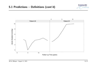
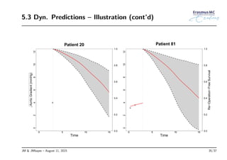
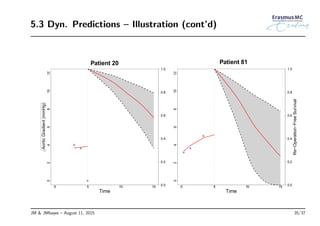
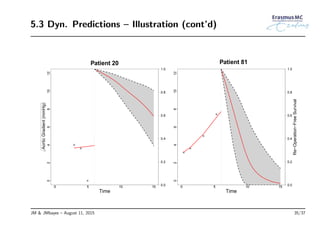
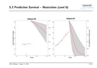
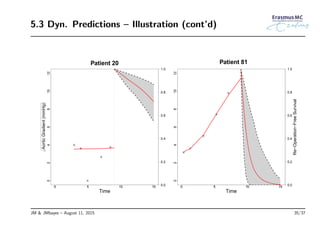
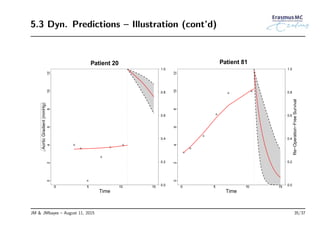
• Individualized predictions of survival probabilities are computed by function
survfitJM() – for example, for Patient 2 from the PBC dataset we have
sfit <- survfitJM(jointFit, newdata = pbc2[pbc2$id == "2", ])
sfit
plot(sfit)
plot(sfit, include.y = TRUE)
JM & JMbayes – August 11, 2015 33/37](https://image.slidesharecdn.com/presjmbayes-150809152353-lva1-app6891/85/JM-and-JMbayes-JSM2015-36-320.jpg)


The document discusses fitting joint models using R packages jm and jmbayes, focusing on longitudinal and time-to-event data analysis. It presents a case study on aortic valve patients and outlines the research questions, joint modeling framework, and software implementation for analyzing the relationships between aortic gradient and survival/re-operation events. The goals are to introduce joint modeling methods and demonstrate the capabilities of the software for statistical analyses in biostatistics.