Download as PDF, PPTX
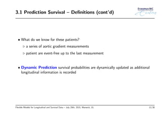


![4.2 Next Visit Time – Model (cont’d)
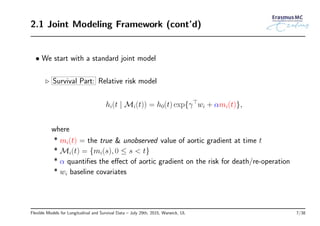
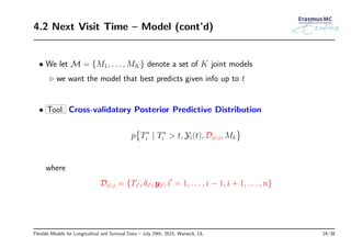
• We let M∗
the true model – then we select the model Mk in the set M that
minimizes the cross-entropy (Commenges et al., Biometrics, 2012):
CEk(t) = E
{
− log
[
p
{
T∗
i | T∗
i > t, Yi(t), Dni, Mk
}]}
where the expectation is wrt [T∗
i | T∗
i > t, Yi(t), Dni, M∗
]
• An estimate that accounts for censoring:
cvDCLk(t) =
1
nt
n∑
i=1
−I(Ti > t) log p
{
Ti, δi | Ti > t, Yi(t), Dni, Mk
}
Flexible Models for Longitudinal and Survival Data – July 29th, 2015, Warwick, UL 25/38](https://image.slidesharecdn.com/presnextvisit-150809152707-lva1-app6891/85/Personalized-Screening-using-Joint-Models-35-320.jpg)
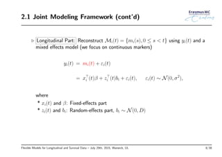
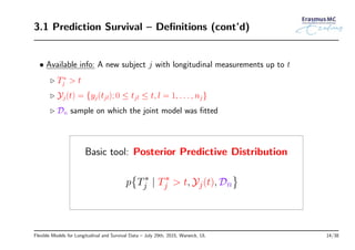
![4.3 Next Visit Time – Timing (cont’d)
• Utility function
U(u | t) = E
{
λ1 log
p
(
T∗
j | T∗
j > u,
{
Yj(t), yj(u)
}
, Dn
)
p{T∗
j | T∗
j > u, Yj(t), Dn}
+λ2 I(T∗
j > u)
}
First term Second term
expectation wrt joint predictive distribution [T∗
j , yj(u) | T∗
j > t, Yj(t), Dn]
◃ First term: expected Kullback-Leibler divergence of posterior predictive
distributions with and without yj(u)
◃ Second term: ‘cost’ of waiting up to u ⇒ increase the risk
Flexible Models for Longitudinal and Survival Data – July 29th, 2015, Warwick, UL 31/38](https://image.slidesharecdn.com/presnextvisit-150809152707-lva1-app6891/85/Personalized-Screening-using-Joint-Models-41-320.jpg)
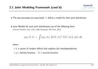
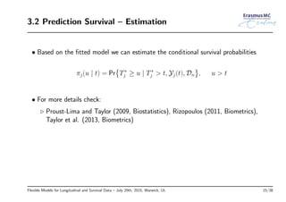
![4.3 Next Visit Time – Timing (cont’d)
• It can be shown that
◃ for any λ1 and λ2,
◃ there exists a constant κ ∈ [0, 1] for which
argmax
u
U(u | t) ⇐⇒ argmax
u
E
{
log
p
(
T∗
j | T∗
j > u,
{
Yj(t), yj(u)
}
, Dn
)
p{T∗
j | T∗
j > u, Yj(t), Dn}
}
subject to the constraint πj(u | t) ≥ κ
Flexible Models for Longitudinal and Survival Data – July 29th, 2015, Warwick, UL 33/38](https://image.slidesharecdn.com/presnextvisit-150809152707-lva1-app6891/85/Personalized-Screening-using-Joint-Models-43-320.jpg)
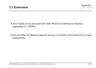
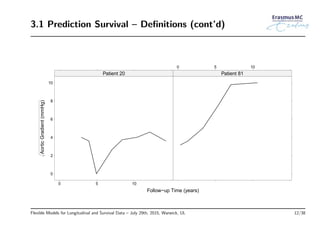
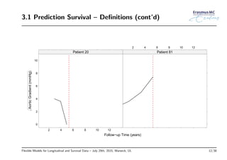
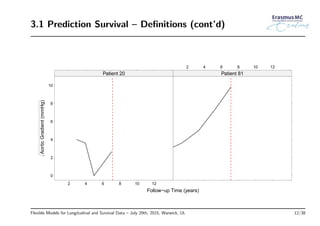
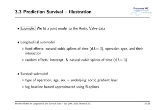
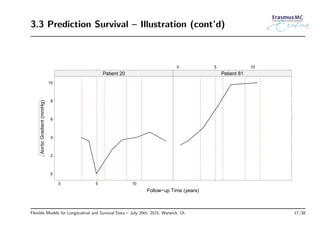
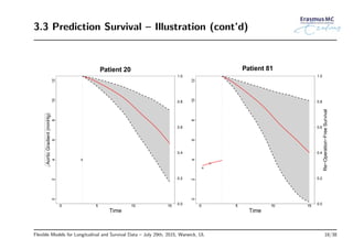
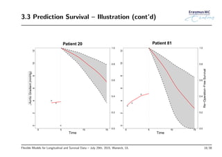
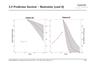
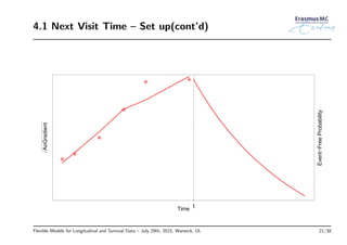
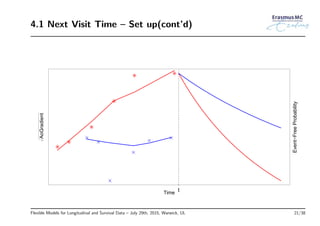
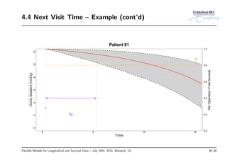
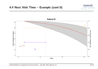
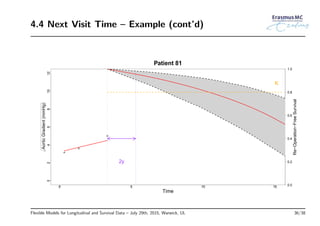
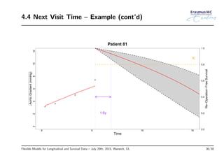
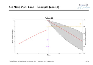
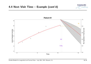
![4.4 Next Visit Time – Example
• Example: We illustrate how for Patient 81 we have seen before
◃ The threshold for the constraint is set to
πj(u | t) ≥ κ = 0.8
◃ After each visit we calculate the optimal timing for the next one using
argmax
u
EKL(u | t) where u ∈ (t, tup
]
and
tup
= min{5, u : πj(u | t) = 0.8}
Flexible Models for Longitudinal and Survival Data – July 29th, 2015, Warwick, UL 35/38](https://image.slidesharecdn.com/presnextvisit-150809152707-lva1-app6891/85/Personalized-Screening-using-Joint-Models-45-320.jpg)


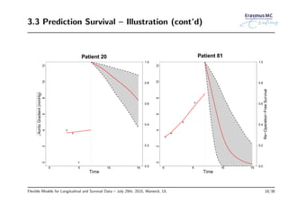
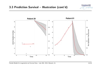
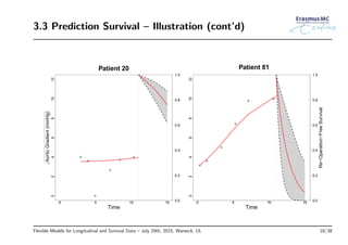
This document presents a study on optimal screening intervals for biomarkers using joint models for longitudinal and survival data, specifically in the context of aortic valve patients. It discusses the importance of personalized medicine and the use of joint models to predict survival and determine optimal timings for patient visits based on aortic gradient measurements. The methodology includes Bayesian estimation and cross-validation approaches for model selection and prediction.