This document summarizes a statistical analysis project using classification and prediction models to analyze charitable donation data. The goals were to 1) build a classification model to identify likely donors to maximize profit, and 2) develop a prediction model for donation amounts based on donor characteristics. Several models were tested on training, validation, and test datasets. The best classification model was a gradient boosting machine with an error rate of 11.4% and projected profit of $11,941.50. The best prediction model was a gradient boosting machine with a mean prediction error of 1.414.

1. STAT 897D – Applied Data Mining and Statistical Learning
Final Team Project on
Analyzing Charitable Donation Data Using
Classification and Prediction Models
Rebecca Ray
Jonathan Fivelsdal
Joana E. Matos
May 1st, 2016

2. 1
INTRODUCTION
Colleges, religions, non-profits and other humanitarian organizations receive charitable donations on
a regular basis. Every one of these organizations could benefit from identifying cost-effective methods
to achieve higher volumes of net profit. In this case study, we consider different data mining models in
order to improve the cost-effectiveness of direct marketing campaigns to previous donors carried out
by a particular charitable organization.
The task of this study is two-fold. The first objective is to build a classification model from the most
recent direct marketing campaign in order to identify likely donors such that the expected net profit is
maximized. The second objective consists of developing a model that will predict donation amounts
based on donor characteristics. For this, we fit a multitude of models to a training subset of the data in
order to identify the most appropriate classification and prediction models.
ANALYSIS
The organization’s entire dataset included 8009 observations. In order to analyze and fit the data to
several models, the entire dataset had been previously split into three groups: a training dataset
comprising of 3984 observations, a validation dataset with 2018 observations, and test dataset
comprising of 2007 observations. The training and validation data used a weighted model, over-
representing the responders so that the training and validation samples have approximately equal
numbers of donors and non-donors. The test dataset has the traditional 10% response rate making it
necessary to adjust the mailing rate to calculate profit correctly.
The outcome variables of interest are DONR (donor and non-donor) and donation amounts (DAMT).
Twenty predictors were considered in our models: REG1-4, HOME, CHLD, HINC, GENF, WRAT, AVHV,
INCM, INCA, PLOW, NPRO, TGIF, LGIF, RGIF, TDON, TLAG and AGIF (to see the details of each variable
please refer to Appendix 1).
An exploratory data analysis checked for missing values in the data set. Finding none, we next visualized
the continuous variables. Histograms and a table of Box-Cox lambda values can be found in the
Appendix (Figure 1. in Appendix 2). Skewed variables AVHV, INCM, INCA, TGIF, LGIF, RGIF, TLAG and
AGIF were log -transformed. A cube root transformation was found to be more suitable to the PLOW
variable. When called for, we also standardized the values in the training data such that each predictor
variable has a mean of 0 and a standard deviation of 1.
Classification
To classify donors into two classes – donor and not-donor, we have made use of multiple resources
learned throughout the course: General additive models (GAM), Logistic Regression (LR), Linear
Discriminant Analysis (LDA), Quadratic Discriminant Analysis (QDA), K-nearest neighbors (KNN),

3. 2
Decision trees, Bagged trees, Random forests, Boosting, and Support Vector Machines (SVM). All these
approaches can be used for classification purposes. Models were compared by classification error
rates, and more importantly based on profit.
Prediction
An array of models were used to find the best prediction model, namely, Linear Regression, Best subset
selection, Ridge regression, Lasso, Gradient Boosting Machine and Random Forest. Cross validation was
employed with several methods to improve model fit. To choose the best prediction models, we have
considered the mean prediction error obtained when fitting the model to the training dataset and the
validation dataset. The model that produced the lowest mean prediction error was chosen.
Once the best classification and prediction models were identified, these models were applied to the
test dataset. The DONR and DAMT variables in this dataset were set to “NA”. The application of the
classification model to the test dataset classified individuals into the DONR variable as donor or
nondonor. Similarly, the prediction model when applied to the test data produced a new variable
DAMT as the predicted Donation Amounts in dollars. Please refer to the file “JEDM-RR-JF.csv” for these
results.
R was used to conduct all the analysis in this report. Some figures are included in the report as an
example. The entire code and additional details can be found in the Appendix.
RESULTS
Classification Models developed for the DONR variable
The first objective of this study was to generate a model that classifies donors in two classes: class 0
and class 1. In order to choose the model that best performs this task, we used two criteria: lowest
classification error rate and highest projected profit. Ideally, projected mailings would also be the
lowest.
Logistic Regression
Logistic regression models will investigate the probability that a certain response will belong to one of
two categories, in this case being a donor or not. The logistic regression model that performed the best
was one that included HINC 2 and excluded PLOW, REG4, and AVHV achieved through backward
elimination. There were others that gave lower AIC scores but when applied to the validation data
produced larger error rates and less profit. With the above-mentioned logistic regression model, the
classification error rate was 34.1%, projected maximum profit was $10,943.50 and projected mailings
were 1,655.

4. 3
Linear Discriminant Analysis (LDA)
Linear Discriminant Analysis models the distribution of the different predictors separately for each of
the response classes and then estimates the probability of a response Y to be in a certain class, given
the predictor X. Here, we found that the best linear discriminant analysis included all variables including
HINC 2. Removal of REG4 which has been the least helpful variable in other models did not improve the
model. Fitting an LDA model to the data resulted in a model with a classification error rate of 19.9%, a
projected profit of $11,620.50 and 1,389 projected mailings (Table 1.). This was quite an improvement
over the logistic regression model above.
Quadratic Discriminant Analysis (QDA)
QDA is very similar to LDA, except that it assumes that each class (donors and not donors in this case)
will have its own covariance matrix. The best QDA also included all variables including the HINC 2. As
in the LDA, removal of REG4 was detrimental to the model, so it was added back in. With the QDA
model, the classification error rate was 23.5%, the projected profit was $11,243.50 and there were
1,418 projected mailings. QDA performed slightly poorer than LDA.
K-Nearest Neighbor (KNN)
KNN is the most non-parametric model of the models created so far. It tries to estimate the distribution
of all predictor variables to come closest to a Bayes classifier. The k values tested were between k=3
and k=14. The model that performed the best was the mode that used k=13 which is less flexible than
the k=3 model.
Generalized Additive Model (GAM)
A smoothing spline was applied to the continuous variables. The best fitting model used a df = 10 and
excluded the variables REG3, REG4, GENF, RGIF, AGIF, and LGIF. Eliminations were made using
backward elimination. This model achieved both the best AIC score and profit amounts of the GAM
candidate models (Figure 1).
Decision Trees: Random Forests, Bagging and Gradient Boosting Model
Random forests have a higher degree of flexibility than more traditional methods such as logistic
regression and linear discriminant analysis and can provide a higher quality of classification than
building a single decision tree. All random forest models in this report build 3500 trees with an
interaction depth of 4. In order to identify a tree with low error, 10-fold cross-validation (CV) was
performed. We concluded that random forests with 10 and 20 predictors displayed the lowest CV error
(0.12 and 0.11, respectively). Even though CV error was slightly higher for the random forest with 10
predictors, the profit and validation error rates were much better. The maximum profit achieved by
the random forest model using 10 predictors was $11,774.50 with 1,254 mailings. Most actual donors
and actual non-donors were correctly classified by the model when applied to the validation data set.
The classification error rate for the model is 13.73%.

5. 4
Figure 1. Expected net profit vs. number of mailings for the Gradient Boosting Machine model: maximum profit
= $11,941.50, number of mailings: 1,214.
When using bagging, the model with 10 predictors also out-performed the model with 20 predictors.
The classification error rate for this model was 16.5%, and the maximum profit was $11,695.50 with
1,308 mailings (Table 1).
For the GBM models, we experimented with different values for shrinkage (0.001 to 0.01) and number
of trees (2,500 to 3,500). The GBM that we found performed the best used 3500 trees, a depth of 4
and a shrinkage of 0.005. For this model, we found that the maximum profit $11,941.50 with 1,214
mailings, and the classification error rate was 11.4% (Table 1). This model out-performed all the
remaining models, in terms of both classification error rate and maximum profit.
We summarize the relevant results for all the classification models in the next table (Table 1). We
observe that the models consisting of decision trees performed much better than the other
classification models, both in terms of classification error rates, but also on the projected maximum
profit. Among the decision trees models, we have found that the gradient boosting model with 3500
trees, a depth of 4 and a shrinkage of 0.005 was the best and it would therefore be our selection.

6. 5
Table 1. Summary of results for the eight chosen classification models. Shown are the classification error rates,
projected mailings and projected profit.
Validation DataValidation DataValidation DataValidation Data
Classification Model for DONRClassification Model for DONRClassification Model for DONRClassification Model for DONR Classification
error rate
Projected
Mailings
Projected
Profit
Logistic RegressionLogistic RegressionLogistic RegressionLogistic Regression 34.1% 1,655 $10,943.50
LDALDALDALDA 19.9% 1,389 $11,620.50
QDAQDAQDAQDA 23.5% 1,418 $11,243.50
KNNKNNKNNKNN 18.4% 1,267 $11,197.50
GAM with df=10GAM with df=10GAM with df=10GAM with df=10 27.8% 1,528 $11,197.50
Decision Trees:Decision Trees:Decision Trees:Decision Trees:
BaggingBaggingBaggingBagging 16.5% 1,308 $11,695.50
Random ForestRandom ForestRandom ForestRandom Forest –––– 10 predictors10 predictors10 predictors10 predictors 13.7% 1,254 $11,774.50
Gradient BoostingGradient BoostingGradient BoostingGradient Boosting 11.4% 1,214 $11,941.50
Prediction Models developed for the DAMT variable
The second goal of this project was to develop a model to predict donation amounts based on the
characteristics of the donors. For this, we chose among our models using the criteria of the lowest
mean prediction error.
Least Squares, Best Subset and Backward Stepwise Regressions
Some benefits of linear regression models are that they have low bias which makes them less prone to
overfitting versus more flexible methods and they are also highly interpretable.
We have performed Least Squares Regression, Best Subset Selection and Backward Stepwise selection.
In order to evaluate these models, we have analyzed the BIC values. Figure 2. Shows the BIC values for
models with different numbers of predictors obtained from fitting a Backwards Stepwise Regression to
the training dataset. All three regressions had similar results and we found that the model with the
lowest BIC contained 8 predictors: REG3, REG4, CHLD, HINC, TGIF, LGIF, RGIF, AGIF.
Least Squares regression had the lowest Mean Prediction error – 1.62. However, the mean prediction
error obtained when fitting a best subsets regression was only slightly bigger (1.63). Please refer to
Table 2. For a summary of these results-

7. 6
Figure 2. BIC values for Backwards Stepwise Regression models with different numbers of predictors.
Support Vector Machine
Support vector machines are called Support Vector regressions (SVR) when used in the prediction
setting. It contains tuning parameters such as cost, gamma and epsilon. In order to fit a SVR model to
the data, we used a fixed gamma value of 0.5 and we performed 10-fold CV to find useful values for
the cost and epsilon parameters. The potential epsilon values we considered in the CV process were
0.1, 0.2 and 0.3 along with potential cost values of 0.01, 1 and 5. After performing 10-fold cross-
validation, it appeared that 0.2 and 1 were promising values for epsilon and cost respectively. Using a
cost value of 1, epsilon value of 0.2 and a gamma value of 0.5, we obtained a support vector regression
model with 1,347 support vectors. When this was applied to the validation set, it resulted in a mean
prediction error of 1.553 and a standard error of 0.174.
Ridge Regression
Ridge regression is similar to least squares, though the coefficients are estimated differently. This
model creates shrinkage of the predictors by using a tuning parameter λ to obtain a set of coefficient
estimates. For this problem, the best λ was 0.1141. The mean prediction error that resulted was 1.63
with a standard error of 0.16.
Lasso Regression
Lasso is another extension of linear regression, which used an alternative procedure of fitting in order
to estimate the coefficients. Given that this procedure is somewhat restrictive, it shrinks some of the
coefficients to exactly zero, unlike what it happens with Ridge. Despite being less flexible than linear
regression, it is more interpretable. We fitted our dataset with a lasso regression model and concluded

8. 7
that the mean prediction error was similar to the ones obtained with the other models (1.62), and the
standard error was 0.16 (Table 2.)
Principal Components Regression
The PCR uses clustering to decrease the dimensionality of the problem space. Looking at the cluster
graph below (Figure 3.), 14 components reduces the mean squared error to the lowest point. This
suggests that there is very little redundancy in the variance accounted for in the prediction variables.
This has been confirmed in earlier regression models. Like the other regression models, the PCR
produced the same mean prediction error (1.63) and standard error (0.16).
Figure 3. Mean Standard Error of Prediction for models with increasing number of components.
Gradient Boosting Machine
Apart from being used in classification problems, GBM models can also be used for prediction. GBM
models that were composed of 3,500 trees appeared to perform well in the classification setting and
so we considered a GBM model with 3,500 trees and a shrinkage value of 0.001 for prediction. When
examining GBM models for classifying donors in the first part, we found that adjusting the shrinkage
value created a higher performing model. After applying different shrinkage values, a GBM model with
3,500 trees and a shrinkage value of 0.01, produced a mean prediction error of 1.414 and a standard
error of 0.162. This GBM model had the lowest mean prediction error considered thus far.

9. 8
Random Forests
Just as gradient boosting machines can be used for both classification and prediction, random forests
can also be used for classification and prediction. After applying the random forest model using 10
predictors to the validation set, we obtained a mean prediction error of 1.679 and a standard error of
0.175. The mean prediction error of this random forest model was higher than every other prediction
model considered thus far except for the GBM model with 3,500 trees and a shrinkage value of 0.001.
The SVR model has a mean prediction error lower than most of the prediction models considered in
this report, however, the mean prediction error of the SVR model is still higher than the GBM model
using 3,500 trees and a shrinkage value of 0.01 (this GBM model has a mean prediction error of 1.414).
PredictionPredictionPredictionPrediction Model for DModel for DModel for DModel for DAMTAMTAMTAMT
Mean
Prediction
Error
Standard
Error
Least Squares RegressionLeast Squares RegressionLeast Squares RegressionLeast Squares Regression 1.62 0.16
Best Subsets RegressionBest Subsets RegressionBest Subsets RegressionBest Subsets Regression 1.63 0.16
Backward Stepwise SelectionBackward Stepwise SelectionBackward Stepwise SelectionBackward Stepwise Selection 1.66 0.16
Support Vector MachineSupport Vector MachineSupport Vector MachineSupport Vector Machine (cost =1, ε = 0.2 and γ = 0.5) 1.55 0.17
Ridge RegressionRidge RegressionRidge RegressionRidge Regression 1.63 0.16
Lasso RegressionLasso RegressionLasso RegressionLasso Regression 1.62 0.16
Principal Components RegressionPrincipal Components RegressionPrincipal Components RegressionPrincipal Components Regression 1.63 0.16
Random ForestRandom ForestRandom ForestRandom Forest (10 predictors)(10 predictors)(10 predictors)(10 predictors) 1.68 0.17
Gradient Boosting MachineGradient Boosting MachineGradient Boosting MachineGradient Boosting Machine (3,500 trees and shrinkage = 0.01) 1.41 0.16
Table 2. Summary of results for the seven prediction models. Shown are the mean prediction
and standard errors.
DISCUSSION
Every single kind of business requires some sort of investment and some kind of return, and its main
objective is to maximize profit. Organizations that receive charitable donations are no different. This
particular charitable organization is looking at a way of maximizing their net profit by capturing likely
donors instead of targeting everyone with their current marketing strategy.
The initial exploratory data analysis revealed that some variables would benefit from being
transformed. In fact, it is common for amounts of money to be lognormally distributed and thus benefit
from a logarithmic transformation. Versions of such variables will be normally distributed or
approximately normally distributed (Mount and Zumel, 1973). Upon analysis, we log-transformed all
the variables in the training set corresponding to an amount of money (AVHV, INCM, INCA, TGIF, LGIF,

10. 9
RGIF and AGIF). We also considered useful to log-transform TLAG and to apply a cube root
transformation to the PLOW variable.
Several models were then fit to the dataset in order to identify the classification model that would
achieve the highest maximum expected net profit value, as well as the predictive model with the lowest
mean prediction error.
From the battery of models we were taught throughout the course, we chose to investigate how
Logistic Regression, LDA, QDA, KNN, GAM with df=10, Decision Trees, Bagging, Random Forest with 10
predictors and Gradient Boosting would perform to tackle the classification of the DONR response
variable. The Gradient Boosting Machine model (GBM) with 3,500 trees and a shrinkage value of 0.05
produced the highest maximum net expected profit ($11,941), together with the lowest classification
error rate (11.4%). Interestingly it is also the model with the lowest number of projected mailings –
1,214. This type of boosting models grows trees sequentially, using information from previously grown
trees. It uses shrinkage in order to shrink or reduce the impact of each additional fitted base-learners,
and it reduces the size of incremental steps. Shrinkage is a classic method of controlling model
complexity through introducing regularization and is used in model techniques such as lasso, ridge
regression and GBMs (Gunn, 1998). It is therefore a method that will tend to keep only the most
relevant variables, and it is a very flexible method in the sense that three different parameters can be
tuned. It has been shown that increasing the value of the shrinkage parameter in a GBM model results
in a more generalizable model (Natekin and Knoll, 2013). Whilst we considered initially a default value
of 0.001, we have concluded later that a shrinkage value of 0.005 yields better results. Another tuning
parameter is the number of trees that the model produces. We have started with a GBM that used
2,500 trees but concluded that increasing this number to 3,500 improved the performance of the
model. This model was therefore the model that we would recommend the charitable organization to
use in order to classify the donors.
In order to develop a prediction model for the DAMT variable, we used the set of tools made available
to us throughout this course that allows to fit a model to a quantitative response: Least Squares
Regression, Best Subsets Regression, Support Vector Machine, Ridge Regression, Lasso Regression,
Principal Components Regression and Gradient Boosting Machine. GBMs are interesting given that they
allow to fit models regardless of whether the response variable is qualitative or quantitative. Also here,
we found that the GBM model with a shrinkage value of 0.01 and 3,400 trees yielded the best results
with the lowest mean prediction error of 1.41 and standard error. Thus, the GBM model with 3,500
trees and shrinkage of 0.01 was used to classify DONR responses in and predict donation amounts
(DAMT responses) in the test dataset (please refer to the file “TeamJ_class_preds.csv” for these
results).
It is interesting to note that this flexibility of GBMs has been previously documented and reported by
Natekin and Knoll (2013) who stated that their “…high flexibility makes the GBMs highly customizable
to any particular data driven task” and that “GBMs have shown considerable success in not only
practical applications, but also in various machine-learning and data-mining challenges.”

11. 10
REFERENCES
Gunn SR (1998). Support Vector Machines for Classification and Regression. University of
Southampton.
James G, Witten D, Hastie T, Tibshirani R. (2015). An Introduction to Statistical Learning with
Applications in R. Springer New York Heidelberg Dordrecht London.
Mount J and Zumel N (2014). Practical Data Science With R. Manning Publication Co.
Natekin A and Knoll A (2013). Gradient boosting machines, a tutorial. Frontier in Neurorobotics, Volume
7, Article 21. (Retrieved from: http://doi.org/10.3389/fnbot.2013.00021).
R Core Team. (2015). R: A Language and Environment for Statistical Computing. R Foundation for
Statistical Computing, Vienna, Austria. (Retrieved from: http://www.R-project.org/)
Course notes for STAT 897D – Applied Data Mining and Statistical Learning. [Online]. [Accessed January
- April 2016]. Available from: < https://onlinecourses.science.psu.edu/stat857/>

12. 11
APPENDIX

13. 12
APPENDIX 1 - VARIABLES
Vars. Description Vars. Description
ID Identification number PLOW % categorized as “low income” in
potential donor’s neighborhood
REG 5 regions indicator variables respectively
called REG1, REG2, REG3 and REG4
NPRO Lifetime number of promotions
received to date
HOME (1 = homeowner, 0 = not a homeowner TGIF Dollar amount of lifetime gifts to date
CHLD Number of children LGIF Dollar amount of largest gift to date
HINC Household income (7 categories) RGIF Dollar amount of most recent gift
GENF Gender (0 = Male, 1 = Female) TDON Number of months since last donation
WRAT Wealth Rating (Wealth rating uses median
family income and population statistics from
each area to index relative within each state.
The segments are denoted 0-9, with 9 being
the highest wealth group and 0 being the
lowest
TLAG Number of months between first and
second gift
AVHV Average Home Value in potential donor’s
neighborhood in $ thousands
AGIF Average dollar amount of gifts to date
INCM Median Family Income in potential donor’s
neighborhood in $ thousands
DONR Classification Response Variable
(1=Donor, 0 = Non-donor)
INCA Average Family Income in potential donor’s
neighborhood in $ thousands
DAMT Prediction Response Variable
(Donation amount in $)

14. 13
APPENDIX 2 – EXPLORATORY DATA ANALYSIS
Figure 1. Histograms for all predictor variables

15. 14
APPENDIX 3 – CODES

16. library(ggplot2)
library(tree) #Use tree package to create classification tree
library(randomForest)
library(nnet)
library(gbm)
library(caret)
library(ggplot2)
library(pbkrtest)
library(glmnet)
library(lme4)
library(Matrix)
library(gam)
library(MASS)
library(leaps)
library(glmnet)
#charity <- read.csv("~/Penn_State/STAT897D/Projects/Final_Project/charity.csv")
#charity <- read.csv("charity.csv")
charity <- read.csv("~/Penn_State/STAT897D/Projects/Final_Project/charity.csv")
#charity <- read.csv("~/Documents/teaching/psu/charity.csv")
#charity <- read.csv("charity.csv")
#A subset of the data without the donr and damt variables
charitySub <- subset(charity,select = -c(donr,damt))
#Check for missing values in the data excluding the donr and damt variables
sum(is.na(charitySub)) #There are no missing data among the other variables
# predictor transformations
charity.t <- charity
#A log transformed version of "avhv" is approximately normally distributed
# versus the untransformed version of "avhv"
charity.t$avhv <- log(charity.t$avhv)
charity.t$incm <- log(charity.t$incm)
charity.t$inca <- log(charity.t$inca)
charity.t$plow <- charity.t$plow^(1/3)
charity.t$tgif <- log(charity.t$tgif)
charity.t$lgif <- log(charity.t$lgif)
charity.t$rgif <- log(charity.t$rgif)
charity.t$tlag <- log(charity.t$tlag)
charity.t$agif <- log(charity.t$agif)
# add further transformations if desired
# for example, some statistical methods can struggle when predictors are highly skewed
# set up data for analysis
#Training Set Section
data.train <- charity.t[charity$part=="train",]
x.train <- data.train[,2:21]
c.train <- data.train[,22] # donr
n.train.c <- length(c.train) # 3984
y.train <- data.train[c.train==1,23] # damt for observations with donr=1
n.train.y <- length(y.train) # 1995
#Validation Set Section
data.valid <- charity.t[charity$part=="valid",]
x.valid <- data.valid[,2:21]
c.valid <- data.valid[,22] # donr
n.valid.c <- length(c.valid) # 2018
y.valid <- data.valid[c.valid==1,23] # damt for observations with donr=1
n.valid.y <- length(y.valid) # 999
#Test Set Section
data.test <- charity.t[charity$part=="test",]
n.test <- dim(data.test)[1] # 2007
x.test <- data.test[,2:21]
#Training Set Mean and Standard Deviation
x.train.mean <- apply(x.train, 2, mean)
x.train.sd <- apply(x.train, 2, sd)
#Standardizing the Variables in the Training Set
x.train.std <- t((t(x.train)-x.train.mean)/x.train.sd) # standardize to have zero mean and unit sd

17. apply(x.train.std, 2, mean) # check zero mean
apply(x.train.std, 2, sd) # check unit sd
#Data Frame for the "donr" variable in the Training Set
data.train.std.c <- data.frame(x.train.std, donr=c.train) # to classify donr
data.train.std.y <- data.frame(x.train.std[c.train==1,], damt=y.train) # to predict damt when donr=1
#Standardizing the Variables in the Validation Set
x.valid.std <- t((t(x.valid)-x.train.mean)/x.train.sd) # standardize using training mean and sd
data.valid.std.c <- data.frame(x.valid.std, donr=c.valid) # to classify donr
#Data Frame for the "donr" variable in the Validation Set
data.valid.std.y <- data.frame(x.valid.std[c.valid==1,], damt=y.valid) # to predict damt when donr=1
#Standardizing the Variables in the Test Set
x.test.std <- t((t(x.test)-x.train.mean)/x.train.sd) # standardize using training mean and sd
data.test.std <- data.frame(x.test.std)
# logistic Regression Model 3 is best
library(MASS)
boxplot(data.train)
model.logistic <- glm(donr ~ reg1 + +reg2 + reg3 + reg4 + home + chld + hinc + I(hinc^2)+genf + wrat +
avhv + incm + inca + plow + npro + tgif + lgif + rgif + tdon + tlag + agif, data.train,
family=binomial("logit"))
summary(model.logistic)
model.logistic1 <- glm(donr ~ reg1 + +reg2 + reg3 + reg4 + home + chld + hinc + I(hinc^2)+genf + wrat +
avhv + incm + inca + npro + tgif + lgif + rgif + tdon + tlag + agif, data.train,
family=binomial("logit"))
summary(model.logistic1)
model.logistic2 <- glm(donr ~ reg1 + +reg2 + reg3 + home + chld + hinc + I(hinc^2)+genf + wrat +
avhv + incm + inca + npro + tgif + lgif + rgif + tdon + tlag + agif, data.train,
family=binomial("logit"))
summary(model.logistic2)
model.logistic3 <- glm(donr ~ reg1 + +reg2 + reg3 + home + chld + hinc + I(hinc^2)+genf + wrat +
rgif + incm + inca + npro + tgif + lgif + tdon + tlag + agif, data.train,
family=binomial("logit"))
summary(model.logistic3)
model.logistic4 <- glm(donr ~ reg1 + +reg2 + home + chld + hinc + I(hinc^2)+genf + wrat +
rgif + incm + inca + npro + tgif + lgif + tdon + tlag + agif, data.train,
family=binomial("logit"))
summary(model.logistic4)
model.logistic5 <- glm(donr ~ reg1 + +reg2 + home + chld + hinc + I(hinc^2)+genf + wrat +
rgif + incm + inca + npro + tgif + tdon + tlag + agif, data.train, family=binomial("logit"))
summary(model.logistic5)
model.logistic6 <- glm(donr ~ reg1 + +reg2 + home + chld + hinc + I(hinc^2)+genf + wrat +
rgif + incm + inca + tgif + tdon + tlag + agif, data.train, family=binomial("logit"))
summary(model.logistic6)
model.logistic7 <- glm(donr ~ reg1 + +reg2 + home + chld + hinc + I(hinc^2)+genf + wrat +
rgif + incm + inca + tgif + tdon + tlag, data.train, family=binomial("logit"))
summary(model.logistic7)
post.valid.logistic <- predict(model.logistic,data.valid.std.c,type="response") # n.valid.c post probs
post.valid.logistic1 <- predict(model.logistic1,data.valid.std.c,type="response") # n.valid.c post probs
post.valid.logistic2 <- predict(model.logistic2,data.valid.std.c,type="response") # n.valid.c post probs
post.valid.logistic3 <- predict(model.logistic3,data.valid.std.c,type="response") # n.valid.c post probs
post.valid.logistic4 <- predict(model.logistic4,data.valid.std.c,type="response") # n.valid.c post probs
post.valid.logistic5 <- predict(model.logistic5,data.valid.std.c,type="response") # n.valid.c post probs
post.valid.logistic6 <- predict(model.logistic6,data.valid.std.c,type="response") # n.valid.c post probs
post.valid.logistic7 <- predict(model.logistic7,data.valid.std.c,type="response") # n.valid.c post probs
# calculate ordered profit function using average donation = $14.50 and mailing cost = $2
profit.logistic <- cumsum(14.5*c.valid[order(post.valid.logistic, decreasing=T)]-2)
plot(profit.logistic) # see how profits change as more mailings are made
n.mail.valid <- which.max(profit.logistic) # number of mailings that maximizes profits
c(n.mail.valid, max(profit.logistic)) # report number of mailings and maximum profit
cutoff.logistic <- sort(post.valid.logistic, decreasing=T)[n.mail.valid+1] # set cutoff based on n.mail.valid
chat.valid.logistic <- ifelse(post.valid.logistic>cutoff.logistic, 1, 0) # mail to everyone above the cutoff
table(chat.valid.logistic, c.valid) # classification table
1-mean(chat.valid.logistic==c.valid)
# True Neg 345 True Pos 983 Miss 34.19% Profit 10937.5
profit.logistic1 <- cumsum(14.5*c.valid[order(post.valid.logistic1, decreasing=T)]-2)
plot(profit.logistic1) # see how profits change as more mailings are made
n.mail.valid <- which.max(profit.logistic1) # number of mailings that maximizes profits
c(n.mail.valid, max(profit.logistic1)) # report number of mailings and maximum profit
cutoff.logistic1 <- sort(post.valid.logistic1, decreasing=T)[n.mail.valid+1] # set cutoff based on n.mail.valid
chat.valid.logistic1 <- ifelse(post.valid.logistic1>cutoff.logistic1, 1, 0) # mail to everyone above the cutoff
table(chat.valid.logistic1, c.valid) # classification table
1-mean(chat.valid.logistic1==c.valid)

18. # True Neg 345 True Pos 983 Miss 34.19% Profit 10939.5
profit.logistic2 <- cumsum(14.5*c.valid[order(post.valid.logistic2, decreasing=T)]-2)
plot(profit.logistic2) # see how profits change as more mailings are made
n.mail.valid <- which.max(profit.logistic2) # number of mailings that maximizes profits
c(n.mail.valid, max(profit.logistic2)) # report number of mailings and maximum profit
cutoff.logistic2 <- sort(post.valid.logistic2, decreasing=T)[n.mail.valid+1] # set cutoff based on n.mail.valid
chat.valid.logistic2 <- ifelse(post.valid.logistic2>cutoff.logistic2, 1, 0) # mail to everyone above the cutoff
table(chat.valid.logistic2, c.valid) # classification table
1-mean(chat.valid.logistic2==c.valid)
# True Neg 345 True Pos 983 Miss 34.19% Profit 10939.5
profit.logistic3 <- cumsum(14.5*c.valid[order(post.valid.logistic3, decreasing=T)]-2)
plot(profit.logistic3) # see how profits change as more mailings are made
n.mail.valid <- which.max(profit.logistic3) # number of mailings that maximizes profits
c(n.mail.valid, max(profit.logistic3)) # report number of mailings and maximum profit
cutoff.logistic3 <- sort(post.valid.logistic3, decreasing=T)[n.mail.valid+1] # set cutoff based on n.mail.valid
chat.valid.logistic3 <- ifelse(post.valid.logistic3>cutoff.logistic3, 1, 0) # mail to everyone above the cutoff
table(chat.valid.logistic3, c.valid) # classification table
1-mean(chat.valid.logistic3==c.valid)
# True Neg 347 True Pos 983 Miss 34.09% Profit 10943.5
profit.logistic4 <- cumsum(14.5*c.valid[order(post.valid.logistic4, decreasing=T)]-2)
plot(profit.logistic4) # see how profits change as more mailings are made
n.mail.valid <- which.max(profit.logistic4) # number of mailings that maximizes profits
c(n.mail.valid, max(profit.logistic4)) # report number of mailings and maximum profit
cutoff.logistic4 <- sort(post.valid.logistic4, decreasing=T)[n.mail.valid+1] # set cutoff based on n.mail.valid
chat.valid.logistic4 <- ifelse(post.valid.logistic4>cutoff.logistic4, 1, 0) # mail to everyone above the cutoff
table(chat.valid.logistic4, c.valid) # classification table
1-mean(chat.valid.logistic4==c.valid)
# True Neg 346 True Pos 983 Miss 34.14% Profit 10941.5
profit.logistic5 <- cumsum(14.5*c.valid[order(post.valid.logistic5, decreasing=T)]-2)
plot(profit.logistic5) # see how profits change as more mailings are made
n.mail.valid <- which.max(profit.logistic5) # number of mailings that maximizes profits
c(n.mail.valid, max(profit.logistic5)) # report number of mailings and maximum profit
cutoff.logistic5 <- sort(post.valid.logistic5, decreasing=T)[n.mail.valid+1] # set cutoff based on n.mail.valid
chat.valid.logistic5 <- ifelse(post.valid.logistic5>cutoff.logistic5, 1, 0) # mail to everyone above the cutoff
table(chat.valid.logistic5, c.valid) # classification table
1-mean(chat.valid.logistic5==c.valid)
# True Neg 345 True Pos 982 Miss 34.24% Profit 10927
profit.logistic6 <- cumsum(14.5*c.valid[order(post.valid.logistic6, decreasing=T)]-2)
plot(profit.logistic6) # see how profits change as more mailings are made
n.mail.valid <- which.max(profit.logistic6) # number of mailings that maximizes profits
c(n.mail.valid, max(profit.logistic6)) # report number of mailings and maximum profit
cutoff.logistic6 <- sort(post.valid.logistic6, decreasing=T)[n.mail.valid+1] # set cutoff based on n.mail.valid
chat.valid.logistic6 <- ifelse(post.valid.logistic6>cutoff.logistic6, 1, 0) # mail to everyone above the cutoff
table(chat.valid.logistic6, c.valid) # classification table
1-mean(chat.valid.logistic6==c.valid)
# True Neg 323 True Pos 986 35.13%
profit.logistic7 <- cumsum(14.5*c.valid[order(post.valid.logistic7, decreasing=T)]-2)
plot(profit.logistic7) # see how profits change as more mailings are made
n.mail.valid <- which.max(profit.logistic7) # number of mailings that maximizes profits
c(n.mail.valid, max(profit.logistic7)) # report number of mailings and maximum profit
cutoff.logistic7 <- sort(post.valid.logistic7, decreasing=T)[n.mail.valid+1] # set cutoff based on n.mail.valid
chat.valid.logistic7 <- ifelse(post.valid.logistic7>cutoff.logistic7, 1, 0) # mail to everyone above the cutoff
table(chat.valid.logistic7, c.valid) # classification table
1-mean(chat.valid.logistic7==c.valid)
# True Neg 324, True Pos 986 35.08% miss
# linear discriminant analysis
library(MASS)
model.lda1 <- lda(donr ~ reg1 +reg2 + reg3 + reg4 + home + chld + hinc + I(hinc^2) + genf + wrat +
avhv + incm + inca + plow + npro + tgif + lgif + rgif + tdon + tlag + agif,
data.train.std.c) # include additional terms on the fly using I()

19. # Note: strictly speaking, LDA should not be used with qualitative predictors,
# but in practice it often is if the goal is simply to find a good predictive model
post.valid.lda1 <- predict(model.lda1, data.valid.std.c)$posterior[,2] # n.valid.c post probs
# calculate ordered profit function using average donation = $14.50 and mailing cost = $2
profit.lda1 <- cumsum(14.5*c.valid[order(post.valid.lda1, decreasing=T)]-2)
plot(profit.lda1) # see how profits change as more mailings are made
n.mail.valid <- which.max(profit.lda1) # number of mailings that maximizes profits
c(n.mail.valid, max(profit.lda1)) # report number of mailings and maximum profit
# 1389.0 11620.5
cutoff.lda1 <- sort(post.valid.lda1, decreasing=T)[n.mail.valid+1] # set cutoff based on n.mail.valid
chat.valid.lda1 <- ifelse(post.valid.lda1>cutoff.lda1, 1, 0) # mail to everyone above the cutoff
table(chat.valid.lda1, c.valid) # classification table
# c.valid
#chat.valid.lda1 0 1
# 0 623 6
# 1 396 993
1-mean(chat.valid.lda1==c.valid) #Error rate
# Quadratic Discriminant Analysis
model.qda <- qda(donr ~ reg1 +reg2 + reg3 + reg4 + home + chld + hinc + I(hinc^2) + genf + wrat +
avhv + incm + inca + plow + npro + tgif + lgif + rgif + tdon + tlag + agif,
data.train.std.c) # include additional terms on the fly using I()
post.valid.qda <- predict(model.qda, data.valid.std.c)$posterior[,2] # n.valid.c post probs
# calculate ordered profit function using average donation = $14.50 and mailing cost = $2
profit.qda <- cumsum(14.5*c.valid[order(post.valid.qda, decreasing=T)]-2)
plot(profit.qda) # see how profits change as more mailings are made
n.mail.valid <- which.max(profit.qda) # number of mailings that maximizes profits
c(n.mail.valid, max(profit.qda)) # report number of mailings and maximum profit
# 1418.0 11243.5
cutoff.qda <- sort(post.valid.qda, decreasing=T)[n.mail.valid+1] # set cutoff based on n.mail.valid
chat.valid.qda <- ifelse(post.valid.qda>cutoff.qda, 1, 0) # mail to everyone above the cutoff
table(chat.valid.qda, c.valid) # classification table
# c.valid
#chat.valid.qda 0 1
# 0 572 28
# 1 447 971
1-mean(chat.valid.qda==c.valid) #Error rate
#K Nearest Neighbors
library(class)
set.seed(1)
post.valid.knn=knn(x.train.std,x.valid.std,c.train,k=13)
# calculate ordered profit function using average donation = $14.50 and mailing cost = $2
profit.knn <- cumsum(14.5*c.valid[order(post.valid.knn, decreasing=T)]-2)
plot(profit.knn) # see how profits change as more mailings are made
n.mail.valid <- which.max(profit.knn) # number of mailings that maximizes profits
c(n.mail.valid, max(profit.knn)) # report number of mailings and maximum profit
# 1267.0 11197.5
table(post.valid.knn, c.valid) # classification table
# c.valid
#chat.valid.knn 0 1
# 0 699 52
# 1 320 947
# check n.mail.valid = 320+947 = 1267
# check profit = 14.5*947-2*1267 = 11197.5
1-mean(post.valid.knn==c.valid) #Error rate
#Mailings and Profit values for different values of k
# k=3 1231 10617

20. # k=8 1248 11018
# k=10 1261.0 11151.5
# k=13 1267.0 11197.5
# k=14 1268.0 11137.5
#GAM
library(gam)
model.gam <- gam(donr ~ reg1 + reg2 + reg3 + reg4 + home + s(chld,df=5)+ s(hinc,df=5) +s(I(hinc^2), df=5)
+ genf + s(wrat,df=5) + s(avhv,df=5) + s(inca,df=5)+ s(plow,df=5) + s(npro,df=5) + s(tgif,df=5)
+ s(lgif,df=5) + s(rgif,df=5) + s(tdon,df=5) + s(tlag,df=5) + s(agif,df=5), data.train,
family=binomial)
summary(model.gam)
model.gam <- gam(donr ~ reg1 + reg2 + reg3 + home + s(chld,df=5)+ s(hinc,df=5) +s(I(hinc^2), df=5)
+ genf + s(wrat,df=5) + s(avhv,df=5) + s(inca,df=5)+ s(plow,df=5) + s(npro,df=5) + s(tgif,df=5)
+ s(lgif,df=5) + s(rgif,df=5) + s(tdon,df=5) + s(tlag,df=5) + s(agif,df=5), data.train,
family=binomial)
summary(model.gam)
model.gam <- gam(donr ~ reg1 + reg2 + reg3 + home + s(chld,df=5)+ s(hinc,df=5) +s(I(hinc^2), df=5)
+ s(wrat,df=5) + s(avhv,df=5) + s(inca,df=5)+ s(plow,df=5) + s(npro,df=5) + s(tgif,df=5)
+ s(lgif,df=5) + s(rgif,df=5) + s(tdon,df=5) + s(tlag,df=5) + s(agif,df=5), data.train,
family=binomial)
summary(model.gam)
model.gam <- gam(donr ~ reg1 + reg2 + home + s(chld,df=5)+ s(hinc,df=5) +s(I(hinc^2), df=5)
+ s(wrat,df=5) + s(avhv,df=5) + s(inca,df=5)+ s(plow,df=5) + s(npro,df=5) + s(tgif,df=5)
+ s(lgif,df=5) + s(rgif,df=5) + s(tdon,df=5) + s(tlag,df=5) + s(agif,df=5), data.train,
family=binomial)
summary(model.gam)
model.gam <- gam(donr ~ reg1 + reg2 + home + s(chld,df=5)+ s(hinc,df=5) +s(I(hinc^2), df=5)
+ s(wrat,df=5) + s(avhv,df=5) + s(inca,df=5)+ s(plow,df=5) + s(npro,df=5) + s(tgif,df=5)
+ s(lgif,df=5) + s(tdon,df=5) + s(tlag,df=5) + s(agif,df=5), data.train, family=binomial)
summary(model.gam)
model.gam <- gam(donr ~ reg1 + reg2 + home + s(chld,df=5)+ s(hinc,df=5) +s(I(hinc^2), df=5)
+ s(wrat,df=5) + s(avhv,df=5) + s(inca,df=5)+ s(plow,df=5) + s(npro,df=5) + s(tgif,df=5)
+ s(lgif,df=5) + s(tdon,df=5) + s(tlag,df=5), data.train, family=binomial)
summary(model.gam)
model.gam <- gam(donr ~ reg1 + reg2 + home + s(chld,df=5)+ s(hinc,df=5) +s(I(hinc^2), df=5)
+ s(wrat,df=5) + s(avhv,df=5) + s(inca,df=5)+ s(plow,df=5) + s(npro,df=5) + s(tgif,df=5)
+ s(tdon,df=5) + s(tlag,df=5), data.train, family=binomial)
summary(model.gam)
post.valid.gam <- predict(model.gam,data.valid.std.c,type="response") # n.valid.c post probs
profit.gam <- cumsum(14.5*c.valid[order(post.valid.gam, decreasing=T)]-2)
plot(profit.gam) # see how profits change as more mailings are made
n.mail.valid <- which.max(profit.gam) # number of mailings that maximizes profits
c(n.mail.valid, max(profit.gam)) # report number of mailings and maximum profit
cutoff.gam <- sort(post.valid.gam, decreasing=T)[n.mail.valid+1] # set cutoff based on n.mail.valid
chat.valid.gam <- ifelse(post.valid.gam>cutoff.gam, 1, 0) # mail to everyone above the cutoff
table(chat.valid.gam, c.valid) # classification table
1-mean(chat.valid.gam==c.valid)
# error rate 21.6% Profit 10461.5 mailings 2012
#GAM df=10
library(gam)
model.gam2 <- gam(donr ~ reg1 + reg2 + home + s(chld,df=10) + s(hinc,df=10) +s(I(hinc^2), df=10)
+ s(wrat,df=10) + s(avhv,df=10) + s(inca,df=10)+ s(plow,df=10) + s(npro,df=10) + s(tgif,df=10)
+ s(tdon,df=10) + s(tlag,df=10), data.train, family=binomial)
summary(model.gam2)
post.valid.gam2 <- predict(model.gam2,data.valid.std.c,type="response") # n.valid.c post probs
profit.gam2 <- cumsum(14.5*c.valid[order(post.valid.gam2, decreasing=T)]-2)
plot(profit.gam2) # see how profits change as more mailings are made
n.mail.valid <- which.max(profit.gam2) # number of mailings that maximizes profits
c(n.mail.valid, max(profit.gam2)) # report number of mailings and maximum profit
cutoff.gam2 <- sort(post.valid.gam2, decreasing=T)[n.mail.valid+1] # set cutoff based on n.mail.valid
chat.valid.gam2 <- ifelse(post.valid.gam2>cutoff.gam2, 1, 0) # mail to everyone above the cutoff
table(chat.valid.gam2, c.valid) # classification table
1-mean(chat.valid.gam2==c.valid)
# 27.8% Profit 11197.5 Mailing 1528
#GAM df=15
library(gam)

21. model.gam <- gam(donr ~ reg1 + reg2 + home + s(chld,df=15)+ s(hinc,df=15)+s(I(hinc^2),df=10)
+ s(wrat,df=15) + s(avhv,df=15) + s(inca,df=15)+ s(plow,df=15) + s(npro,df=15) + s(tgif,df=15)
+ s(tdon,df=15) + s(tlag,df=15), data.train, family=binomial)
summary(model.gam)
post.valid.gam <- predict(model.gam,data.valid.std.c,type="response") # n.valid.c post probs
profit.gam <- cumsum(14.5*c.valid[order(post.valid.gam, decreasing=T)]-2)
plot(profit.gam) # see how profits change as more mailings are made
n.mail.valid <- which.max(profit.gam) # number of mailings that maximizes profits
c(n.mail.valid, max(profit.gam)) # report number of mailings and maximum profit
cutoff.gam <- sort(post.valid.gam, decreasing=T)[n.mail.valid+1] # set cutoff based on n.mail.valid
chat.valid.gam <- ifelse(post.valid.gam>cutoff.gam, 1, 0) # mail to everyone above the cutoff
table(chat.valid.gam, c.valid) # classification table
1-mean(chat.valid.gam==c.valid)
# errror rate 41.1 Profit 10764.5 Mailings 1817
#GAM df=15
library(gam)
model.gam <- gam(donr ~ reg1 + reg2 + reg3 + reg4 + home + s(chld,df=20)+ s(hinc,df=20)
+ genf + s(wrat,df=20) + s(avhv,df=20) + s(inca,df=20)+ s(plow,df=20) + s(npro,df=20) +
s(tgif,df=20)
+ s(lgif,df=20) + s(rgif,df=20) + s(tdon,df=20) + s(tlag,df=20) + s(agif,df=20), data.train,
family=binomial)
summary(model.gam)
post.valid.gam <- predict(model.gam,data.valid.std.c,type="response") # n.valid.c post probs
profit.gam <- cumsum(14.5*c.valid[order(post.valid.gam, decreasing=T)]-2)
plot(profit.gam) # see how profits change as more mailings are made
n.mail.valid <- which.max(profit.gam) # number of mailings that maximizes profits
c(n.mail.valid, max(profit.gam)) # report number of mailings and maximum profit
cutoff.gam <- sort(post.valid.gam, decreasing=T)[n.mail.valid+1] # set cutoff based on n.mail.valid
chat.valid.gam <- ifelse(post.valid.gam>cutoff.gam, 1, 0) # mail to everyone above the cutoff
table(chat.valid.gam, c.valid) # classification table
1-mean(chat.valid.gam==c.valid)
#error rate 48.6% Profit 10517 Mailing 1977
#############################
#Random Forests for Classification
#############################
library(randomForest)
#Possible Predictors for the random forest
data.train.std.c.predictors <- data.train.std.c[,names(data.train.std.c)!="donr"]
#This code evaluates the performance of random forests using different numbers
#of predictors by means of 10 fold cross-validation
rf.cv.results <- rfcv(data.train.std.c.predictors, as.factor(data.train.std.c$donr), cv.fold=10)
with(rf.cv.results,plot(n.var,error.cv,main = "Random Forest CV Error Vs. Number of Predictors", xlab = "Number of
Predictors",
ylab = "CV Error",
type="b",lwd=5,col="red"))
#Table of number of the number of predictors versus errors in random forest
random.forest.error <- rbind(rf.cv.results$n.var,rf.cv.results$error.cv)
rownames(random.forest.error) <- c("Number of Predictors","Random Forest Error")
random.forest.error
#The minimum cross-validated error for a random forest is the random forest
#with 20 predictors. The CV error for a random forest using 20 predictors is 0.11
# and the CV error for a random forest using 10 predictors is 0.12. Since the

22. # CV error is not that much higher for the random forest with 10 predictors
# than the random forest using 20 predictors, we will first use a random forest
# using 10 predictors.
################################
#Random Forest Using 10 Predictors
################################
require(randomForest)
set.seed(1) #Seed for the random forest that uses 10 predictors
rf.charity.10 <- randomForest(x = data.train.std.c.predictors
,y=as.factor(data.train.std.c$donr),
mtry=10)
rf.charity.10.posterior.valid <- predict(rf.charity.10, data.valid.std.c, type="prob")[,2] # n.valid post probs
profit.charity.RF.10 <- cumsum(14.5*c.valid[order(rf.charity.10.posterior.valid, decreasing=T)]-2)
n.mail.valid <- which.max(profit.charity.RF.10 ) # number of mailings that maximizes profits
c(n.mail.valid, max(profit.charity.RF.10)) # report number of mailings and maximum profit
cutoff.charity.10 <- sort(rf.charity.10.posterior.valid, decreasing=T)[n.mail.valid+1] # set cutoff based on
n.mail.valid
chat.valid.charity.10 <- ifelse(rf.charity.10.posterior.valid>cutoff.charity.10, 1, 0) # mail to everyone above the
cutoff
table(chat.valid.charity.10, c.valid) # classification table
#Classification Matrix
#0 1
#0 760 18
#1 259 981
################################
#Bag - (Random Forest using all 20 possible predictors)
################################
require(randomForest)
set.seed(1)
bag.charity <- randomForest(x = data.train.std.c.predictors
,y=as.factor(data.train.std.c$donr),
mtry=20)
bag.charity.posterior.valid <- predict(bag.charity, data.valid.std.c, type="prob")[,2] # n.valid post probs
profit.charity.bag <- cumsum(14.5*c.valid[order(bag.charity.posterior.valid, decreasing=T)]-2)
n.mail.valid <- which.max(profit.charity.bag ) # number of mailings that maximizes profits
c(n.mail.valid, max(profit.charity.bag)) # report number of mailings and maximum profit
#1308 mailings and Maximum Profit $11,695.50
cutoff.bag <- sort(bag.charity.posterior.valid, decreasing=T)[n.mail.valid+1] # set cutoff based on n.mail.valid
chat.valid.bag <- ifelse(bag.charity.posterior.valid >cutoff.bag, 1, 0) # mail to everyone above the cutoff
table(chat.valid.bag, c.valid) # classification table
# Classification Matrix
#0 1
#0 699 13
#1 320 986
#Comparision of the random forest that uses all 20 predictors (the bag)
#Versus the random forest that uses 10 predictors.
# The maximum profit produced by the random forest using 10 predictors
# is $11,744.50 while the maximum profit produced by the random forest
# using all 20 predictors is $11,695.50. The number of mailings required
# for the maximum profit produced by the random forest using 10 predictors
# is 1,240 mailings while the number of mailings required for the maximum profit
# produced by the bag model (random forest using all 20 predictors)
# is 1,308 mailings.
#Gradient Boosting Machine (GBM) - Section

23. library(gbm)
set.seed(1)
#GBM with 2,500 trees
boost.charity <- gbm(donr~.,
data= data.train.std.c,
distribution = "bernoulli",n.trees=2500,interaction.depth=5)
yhat.boost.charity <- predict(boost.charity,newdata=data.valid.std.c,
n.trees=2500)
mean((yhat.boost.charity - data.valid.std.y)^2)
#Validation Set MSE = 12.64
boost.charity.posterior.valid <- predict(boost.charity,n.trees=2500, data.valid.std.c, type="response") # n.valid
post probs
profit.charity.GBM <- cumsum(14.5*c.valid[order(boost.charity.posterior.valid, decreasing=T)]-2)
plot(profit.charity.GBM ) # see how profits change as more mailings are made
n.mail.valid <- which.max(profit.charity.GBM ) # number of mailings that maximizes profits
c(n.mail.valid, max(profit.charity.GBM )) # report number of mailings and maximum profit
#Send out 1280 mailing and maximum profit: $11,737
cutoff.gbm <- sort(boost.charity.posterior.valid , decreasing=T)[n.mail.valid+1] # set cutoff based on n.mail.valid
chat.valid.gbm <- ifelse(boost.charity.posterior.valid >cutoff.gbm, 1, 0) # mail to everyone above the cutoff
table(chat.valid.gbm, c.valid) # classification table
#Confusion Matrix for GBM with 2,500 trees
# 0 1
#0 725 13
#1 294 986
#GBM with 3,500 trees
set.seed(1)
boost.charity.3500 <- gbm(donr~.,
data= data.train.std.c,
distribution = "bernoulli",n.trees=3500,interaction.depth=5)
yhat.boost.charity.3500 <- predict(boost.charity.3500,newdata=data.valid.std.c,
n.trees=3500)
mean((yhat.boost.charity.3500 - data.valid.std.y)^2)
#Validation Set MSE = 13.37
boost.charity.posterior.valid.3500 <- predict(boost.charity.3500,n.trees=3500, data.valid.std.c, type="response") #
n.valid post probs
profit.charity.GBM.3500 <- cumsum(14.5*c.valid[order(boost.charity.posterior.valid.3500, decreasing=T)]-2)
plot(profit.charity.GBM.3500 ) # see how profits change as more mailings are made
n.mail.valid <- which.max(profit.charity.GBM.3500 ) # number of mailings that maximizes profits
c(n.mail.valid, max(profit.charity.GBM.3500 )) # report number of mailings and maximum profit
#Send out 1300 mailing and maximum profit: $11,784.00
cutoff.gbm.3500 <- sort(boost.charity.posterior.valid.3500 , decreasing=T)[n.mail.valid+1] # set cutoff based on
n.mail.valid
chat.valid.gbm.3500 <- ifelse(boost.charity.posterior.valid.3500 >cutoff.gbm.3500, 1, 0) # mail to everyone above the
cutoff
table(chat.valid.gbm.3500, c.valid) # classification table
#Confusion Matrix for GBM with 3500 trees with shrinkage = 0.001
# 0 1
#0 711 7
#1 308 992
require(gbm)
set.seed(1)
boost.charity.3500.hundreth.Class <- gbm(donr~.,

24. data= data.train.std.c,
distribution = "bernoulli",n.trees=3500,interaction.depth=4,
shrinkage = 0.005)
yhat.boost.charity.3500.hundreth.Class <- predict(boost.charity.3500.hundreth.Class,newdata=data.valid.std.c,
n.trees=3500)
mean((yhat.boost.charity.3500.hundreth.Class - data.valid.std.y)^2)
#Validation Set MSE = 23.02
boost.charity.posterior.valid.3500.hundreth.Class <- predict(boost.charity.3500.hundreth.Class,n.trees=3500,
data.valid.std.c, type="response") # n.valid post probs
profit.charity.GBM.3500.hundreth.Class <-
cumsum(14.5*c.valid[order(boost.charity.posterior.valid.3500.hundreth.Class, decreasing=T)]-2)
plot(profit.charity.GBM.3500.hundreth.Class) # see how profits change as more mailings are made
n.mail.valid <- which.max(profit.charity.GBM.3500.hundreth.Class) # number of mailings that maximizes profits
c(n.mail.valid, max(profit.charity.GBM.3500.hundreth.Class)) # report number of mailings and maximum profit
#Send out 1214 mailing and maximum profit: $11,941.50
cutoff.gbm.3500.hundreth.Class <- sort(boost.charity.posterior.valid.3500.hundreth.Class , decreasing=T)
[n.mail.valid+1] # set cutoff based on n.mail.valid
chat.valid.gbm.3500.hundreth.Class <- ifelse(boost.charity.posterior.valid.3500.hundreth.Class
>cutoff.gbm.3500.hundreth.Class, 1, 0) # mail to everyone above the cutoff
table(chat.valid.gbm.3500.hundreth.Class, c.valid) # classification table
#Confusion Matrix for GBM with 3500 trees with shrinkage = 0.01
# 0 1
#0 796 8
#1 223 991
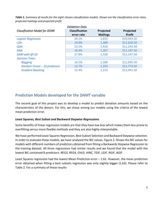
## Prediction Modeling ##
# Multiple regression
model.ls1 <- lm(damt ~ reg1 + reg2 + reg3 + reg4 + home + chld + hinc + genf + wrat +
avhv + incm + inca + plow + npro + tgif + lgif + rgif + tdon + tlag + agif,
data.train.std.y)
pred.valid.ls1 <- predict(model.ls1, newdata = data.valid.std.y) # validation predictions
mean((y.valid - pred.valid.ls1)^2) # mean prediction error
# 1.621358
sd((y.valid - pred.valid.ls1)^2)/sqrt(n.valid.y) # std error
# 0.1609862
# drop wrat, npro, inca
model.ls2 <- lm(damt ~ reg1 + reg2 + reg3 + reg4 + home + chld + hinc + genf +
avhv + incm + plow + tgif + lgif + rgif + tdon + tlag + agif,
data.train.std.y)
pred.valid.ls2 <- predict(model.ls2, newdata = data.valid.std.y) # validation predictions
mean((y.valid - pred.valid.ls2)^2) # mean prediction error
# 1.621898
sd((y.valid - pred.valid.ls2)^2)/sqrt(n.valid.y) # std error
# 0.1608288
# Best Subset, Backwards Stepwise Regression
library(leaps)
charity.sub.reg.back_step <- regsubsets(damt ~.,data.train.std.y,method = "backward", nvmax= 20)
plot(charity.sub.reg.back_step,scale="bic")
#reg3,reg4,home,chld,hinc,incm,tgif, lgif, rgif and agif
#Checked forwards stepwise, same variables returned for minimum bic
#Prediction Model #1
#Least Squares Regression Model - Using predcitors from backward stepwise regression
model.pred.model.1 <- lm(damt ~ reg3 + reg4 + home + chld + hinc + incm + tgif + lgif + rgif + agif,
data = data.train.std.y)
pred.valid.model1 <- predict(model.pred.model.1, newdata = data.valid.std.y) # validation predictions

25. mean((y.valid - pred.valid.model1)^2) # mean prediction error
# 1.628554
sd((y.valid - pred.valid.model1)^2)/sqrt(n.valid.y) # std error
# 0.1603296
charity.sub.reg.best <- regsubsets(damt ~.,data.train.std.y,nvmax= 20)
plot(charity.sub.reg.best,scale="bic")
#reg3,reg4,home,chld,hinc,incm,tgif, lgif, rgif and agif
#Same variables as backwards stepwise
#Principal Components Regression
library(pls)
set.seed(1)
pcr.fit=pcr(damt~.,data=data.train.std.y,scale=TRUE,validation="CV")
validationplot(pcr.fit,val.type="MSEP")
pred.valid.pcr=predict(pcr.fit,data.valid.std.y,ncomp=15)
mean((pred.valid.pcr-y.valid)^2)
# 1.630981
sd((y.valid - pred.valid.pcr)^2)/sqrt(n.valid.y) # std error
#0.1609462
#Support Vector Machine (SVM)
library(e1071)
set.seed(1)
svm.charity <- svm(damt ~.,kernel = "radial",data = data.train.std.y)
pred.valid.SVM.model1 <- predict(svm.charity,newdata=data.valid.std.y)
mean((y.valid - pred.valid.SVM.model1)^2) # mean prediction error
# 1.566
sd((y.valid - pred.valid.SVM.model1)^2)/sqrt(n.valid.y) # std error
# 0.175
set.seed(1)
#10-fold cross validation for SVM using the default gamma of 0.5
# and using varying values of epsilon and cost
charity.svm.tune <- tune(svm,damt~.,kernel = "radial",data=data.train.std.y,
ranges = list(epsilon = c(0.1,0.2,0.3), cost = c(0.01,1,5)))
summary(charity.svm.tune)
#The SVM model has an epsilon of 0.2, a cost of 1 and a gamma of 0.5
svm.charity1 <- charity.svm.tune$best.model
#For the SVM chosen; cost = 1, gamma =0.05 and epsilon=0.2
#There are 1,345 support vectors
summary(charity.svm.tune$best.model)
pred.valid.SVM.model <- predict(svm.charity1,newdata=data.valid.std.y)
mean((y.valid - pred.valid.SVM.model)^2) # mean prediction error
# 1.552217
sd((y.valid - pred.valid.SVM.model)^2)/sqrt(n.valid.y) # std error
# 0.1736719
library(glmnet)
x=model.matrix(damt~.,data.train.std.y)
y=y.train
grid=10^seq(10,-2,length=100)
ridge.mod=glmnet(x,y,alpha=0,lambda=grid)
dim(coef(ridge.mod))
set.seed(1)
cv.out=cv.glmnet(x,y,alpha=0)

26. bestlam=cv.out$lambda.min
valid.mm=model.matrix(damt~.,data.valid.std.y)
pred.valid.ridge=predict(ridge.mod,s=bestlam,newx=valid.mm)
mean((y.valid - pred.valid.ridge)^2) # mean prediction error
# 1.627418
sd((y.valid - pred.valid.ridge)^2)/sqrt(n.valid.y) # std error
# 0.1624537
#Lasso
lasso.mod=glmnet(x,y,alpha=1,lambda=grid)
set.seed(1)
cv.out=cv.glmnet(x,y,alpha=1)
bestlam=cv.out$lambda.min
pred.valid.lasso=predict(lasso.mod,s=bestlam,newx=valid.mm)
mean((y.valid - pred.valid.lasso)^2) # mean prediction error
# 1.622664
sd((y.valid - pred.valid.lasso)^2)/sqrt(n.valid.y) # std error
# 0.1608984
#GBM with 3,500 trees - shrinkage = 0.001
set.seed(1)
#Use Gaussian distribution for regression - 3,500 trees; shrinkage = 0.001
boost.charity.Pred.3500 <- gbm(damt~.,
data= data.train.std.y,
distribution = "gaussian",n.trees=3500,interaction.depth=4)
pred.valid.GBM.model1 <- predict(boost.charity.Pred.3500,newdata=data.valid.std.y,
n.trees=3500)
mean((y.valid - pred.valid.GBM.model1)^2) # mean prediction error
# 1.72
sd((y.valid - pred.valid.GBM.model1)^2)/sqrt(n.valid.y) # std error
# 0.17
#Prediction Model 3 - Gradient Boosting Machine (GBM) With 3,500 trees
#GBM with 3,500 trees - shrinkage = 0.01
set.seed(1)
#Use Gaussian distribution for regression - 3,500 trees; shrinkage = 0.01
boost.charity.3500.hundreth.Pred <- gbm(damt~.,
data= data.train.std.y,
distribution = "gaussian",n.trees=3500,interaction.depth=4,
shrinkage=0.01)
pred.valid.GBM.model2 <- predict(boost.charity.3500.hundreth.Pred,newdata=data.valid.std.y,
n.trees=3500)
mean((y.valid - pred.valid.GBM.model2)^2) # mean prediction error
# 1.413
sd((y.valid - pred.valid.GBM.model2)^2)/sqrt(n.valid.y) # std error
# 0.162
##################################################################################
# select GBM with 3,500 trees and shrinkage = 0.05 (with Bernoulli Distribution)
#since it has maximum profit in the validation sample
post.test <- predict(boost.charity.3500.hundreth.Class,n.trees=3500, data.test.std, type="response") # post probs for
test data
# Oversampling adjustment for calculating number of mailings for test set
n.mail.valid <- which.max(profit.charity.GBM.3500.hundreth.Class)
tr.rate <- .1 # typical response rate is .1
vr.rate <- .5 # whereas validation response rate is .5
adj.test.1 <- (n.mail.valid/n.valid.c)/(vr.rate/tr.rate) # adjustment for mail yes
adj.test.0 <- ((n.valid.c-n.mail.valid)/n.valid.c)/((1-vr.rate)/(1-tr.rate)) # adjustment for mail no
adj.test <- adj.test.1/(adj.test.1+adj.test.0) # scale into a proportion
n.mail.test <- round(n.test*adj.test, 0) # calculate number of mailings for test set

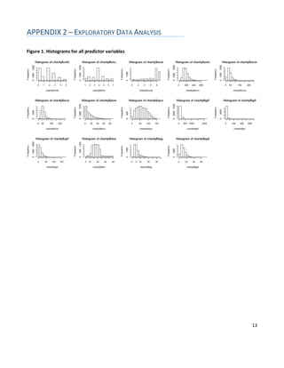
27. cutoff.test <- sort(post.test, decreasing=T)[n.mail.test+1] # set cutoff based on n.mail.test
chat.test <- ifelse(post.test>cutoff.test, 1, 0) # mail to everyone above the cutoff
table(chat.test)
# 0 1
# 1719 288
# based on this model we'll mail to the 288 highest posterior probabilities
# See below for saving chat.test into a file for submission
# select GBM with 3,500 trees and shrinkage = 0.01 (with Gaussian Distribution)
#since it has minimum mean prediction error in the validation sample
yhat.test <- predict(boost.charity.3500.hundreth.Pred,n.trees = 3500, newdata = data.test.std) # test predictions
# Save final results for both classification and regression
length(chat.test) # check length = 2007
length(yhat.test) # check length = 2007
chat.test[1:10] # check this consists of 0s and 1s
yhat.test[1:10] # check this consists of plausible predictions of damt
ip <- data.frame(chat=chat.test, yhat=yhat.test) # data frame with two variables: chat and yhat
write.csv(ip, file="JEDM-RR-JF.csv",
row.names=FALSE) # use group member initials for file name
# submit the csv file in Angel for evaluation based on actual test donr and damt values