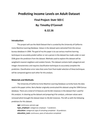
Predicting	
  Income	
  Levels	
  on	
  Adult	
  Dataset	
  
Final	
  Project:	
  Statr	
  503	
  C	
  
By:	
  Timothy	
  O’Connell	
  
6.12.16	


Introduction:	
  	
  
This	
  project	
  will	
  use	
  the	
  Adult	
  Dataset	
  that	
  is	
  curated	
  by	
  the	
  University	
  of	
  California	
  
Irvine	
  Machine	
  Learning	
  Database.	
  Values	
  in	
  the	
  dataset	
  were	
  extracted	
  from	
  the	
  census	
  
bureau	
  database	
  in	
  1994.	
  The	
  goal	
  of	
  my	
  this	
  paper	
  is	
  to	
  use	
  various	
  machine	
  learning	
  
techniques	
  to	
  accurately	
  predict	
  wither	
  or	
  not	
  a	
  person	
  in	
  the	
  dataset	
  has	
  made	
  under	
  or	
  over	
  
$50k	
  given	
  the	
  predictors	
  from	
  the	
  dataset.	
  Methods	
  used	
  to	
  explore	
  this	
  dataset	
  will	
  be	
  
weighted	
  k-­‐nearest	
  neighbors	
  and	
  random	
  forests.	
  This	
  dataset	
  contains	
  both	
  categorical	
  and	
  
integer	
  characteristics	
  and	
  requires	
  classification	
  techniques	
  to	
  accurately	
  complete	
  the	
  
prediction.	
  Classification	
  error	
  rates	
  that	
  come	
  from	
  final	
  model	
  selection	
  of	
  these	
  techniques	
  
will	
  be	
  compared	
  against	
  each	
  other	
  for	
  this	
  analysis.	


Materials	
  and	
  Methods:	
  
The	
  University	
  of	
  California	
  Irvine	
  Machine	
  Learning	
  Database	
  currently	
  hosts	
  the	
  data	
  
used	
  in	
  this	
  paper	
  online.	
  Barry	
  Becker	
  originally	
  constructed	
  this	
  dataset	
  using	
  the	
  1994	
  Census	
  
database.	
  There	
  are	
  a	
  total	
  of	
  15	
  features	
  and	
  32,561	
  instances	
  in	
  the	
  dataset	
  that	
  I	
  used	
  for	
  
this	
  analysis.	
  In	
  cleaning	
  up	
  the	
  dataset	
  and	
  preparing	
  it	
  for	
  analysis,	
  unknown	
  values	
  were	
  
removed	
  which	
  brought	
  the	
  dataset	
  down	
  to	
  30,162	
  instances.	
  This	
  left	
  us	
  with	
  the	
  following	
  
predictors	
  for	
  this	
  dataset.	
  	
  
age:	
  continuous;	
  persons	
  age	
  
type_employer:	
  categorical;	
  employer	
  -­‐	
  7	
  predictors	
  
education:	
  categorical;	
  type	
  of	
  schooling	
  completed	
  -­‐	
  16	
  predictors	
  
education_num:	
  continuous;	
  years	
  of	
  education	
  completed	
  
marital:	
  categorical;	
  persons	
  marital	
  status	
  -­‐	
  7	
  predictors	
  
occupation:	
  categorical;	
  job	
  type	
  –	
  14	
  predictors	
  
relationship:	
  categorical;	
  relationship	
  status	
  –	
  5	
  predictors	
  
race:	
  categorical;	
  persons	
  race	
  -­‐	
  5	
  predictors	
  
sex:	
  binomial	
  persons	
  sex	
  -­‐	
  Male,	
  Female	
  
capital_gain:	
  continuous;	
  capital	
  gains	
  
calital_loss:	
  continuous;	
  capital	
  losses	
  
hr_per_week:	
  continuous;	
  hours	
  person	
  worked	
  per	
  week	
  
income:	
  binomial;	
  income	
  level	
  -­‐	
  above	
  $50k,	
  below	
  $50k	
  
country:	
  categorical	
  -­‐	
  5	
  predictors	
  (see	
  explanation	
  below)	
  	
  
fnlwgt:	
  continuous;	
  predictor	
  that	
  was	
  removed	
  from	
  dataset	
  (see	
  below)	


While	
  processing	
  the	
  data	
  one	
  major	
  categorical	
  choice	
  was	
  made	
  to	
  the	
  country	
  
predictor.	
  The	
  United	
  States	
  was	
  the	
  overwhelming	
  majority	
  (27,518/30,162	
  =	
  ~	
  91.2%)	
  of	
  the	
  
country	
  predictor.	
  To	
  help	
  legitimize	
  this	
  predictor	
  countries	
  were	
  grouped	
  into	
  their	
  
geographical	
  regions	
  (Asia,	
  Canada,	
  Europe,	
  Latin-­‐America,	
  Middle-­‐East,	
  and	
  United	
  States)	
  to	
  
help	
  stabilize	
  this	
  predictor	
  and	
  brought	
  it	
  down	
  from	
  41	
  to	
  5	
  values.	
  The	
  fnlwgt	
  instance	
  in	
  this	
  
dataset	
  represents	
  what	
  the	
  census	
  bureau	
  believed	
  the	
  number	
  of	
  people	
  that	
  observation	
  
represents.	
  It	
  was	
  removed	
  from	
  this	
  analysis	
  because	
  the	
  goal	
  of	
  this	
  paper	
  is	
  not	
  to	
  delve	
  into	
  
tangible,	
  usable	
  results,	
  but	
  rather	
  to	
  compare	
  classification	
  prediction	
  methods	
  and	
  explore	
  
the	
  effects	
  of	
  tuning	
  parameters	
  within	
  these	
  methods.	


To	
  prep	
  the	
  dataset	
  for	
  machine	
  learning/prediction	
  we	
  need	
  to	
  split	
  the	
  data	
  into	
  
training	
  and	
  testing	
  sets.	
  I	
  chose	
  to	
  split	
  the	
  data	
  by	
  20%	
  and	
  80%	
  margins,	
  leaving	
  20%	
  of	
  the	
  
data	
  for	
  the	
  test	
  dataset,	
  a	
  data	
  frame	
  with	
  6,032	
  instances;	
  and	
  the	
  remaining	
  80%	
  delegated	
  
to	
  the	
  training	
  dataset,	
  a	
  dataset	
  with	
  24,130	
  instances.	
  To	
  get	
  a	
  general	
  idea	
  of	
  what	
  was	
  going	
  
on	
  within	
  this	
  dataset	
  we	
  did	
  some	
  very	
  simple	
  visualizations	
  and	
  looked	
  at	
  basic	
  linear	
  models.	
  
Three	
  of	
  the	
  more	
  prominent	
  predictors	
  are	
  shown	
  in	
  box	
  plots	
  below	
  (Figure	
  1.1).	
  As	
  can	
  be	
  
seen,	
  in	
  each	
  of	
  the	
  three	
  boxplots	
  below,	
  education,	
  age	
  and	
  hours	
  worked	
  per	
  week	
  seem	
  to	
  
correlate	
  with	
  higher	
  earnings	
  and	
  may	
  play	
  a	
  significant	
  role	
  as	
  predictors.	
  Our	
  basic	
  linear	
  
model	
  also	
  showed	
  that	
  these	
  were	
  significant	
  in	
  a	
  very	
  basic	
  linear	
  model;	
  and	
  that	
  race,	
  
country	
  (after	
  the	
  transformations)	
  and	
  marital	
  status	
  may	
  not	
  be	
  as	
  important	
  of	
  income	
  level	
  
predictors.	
  	
  
Lastly,	
  it	
  came	
  to	
  our	
  attention	
  that	
  there	
  was	
  an	
  extremely	
  high	
  correlation	
  between	
  
the	
  education	
  and	
  the	
  education_num	
  predictors	
  as	
  education	
  is	
  essentially	
  a	
  categorical	
  
version	
  of	
  education_num.	
  When	
  we	
  move	
  onto	
  model	
  selection,	
  one	
  of	
  these	
  will	
  be	
  removed	
  
from	
  the	
  datasets.	


(Figure	
  1.1)	


Results	
  
	
   The	
  adult	
  dataset	
  has	
  both	
  continuous	
  and	
  categorical	
  attributes.	
  For	
  the	
  limited	
  scope	
  
of	
  this	
  analysis	
  I	
  chose	
  to	
  used	
  the	
  “Weighted	
  k	
  Nearest	
  Neighbors”	
  and	
  “randomForests”	
  
packages	
  in	
  R	
  for	
  this	
  prediction	
  analysis.	


Weighted	
  k	
  Nearest	
  Neighbors:	
  
	
   Applying	
  the	
  weighted	
  k	
  nearest	
  neighbors	
  classification	
  and	
  clustering	
  package,	
  we	
  
started	
  with	
  the	
  “train.kknn”	
  function	
  and	
  applied	
  it	
  to	
  our	
  training	
  dataset.	
  Our	
  first	
  step	
  was	
  
to	
  run	
  the	
  function	
  on	
  the	
  entire	
  dataset	
  predicting	
  income,	
  minus	
  the	
  perfectly	
  correlated	
  
education_num	
  and	
  fnlwgt	
  predictors	
  that	
  were	
  removed.	
  We	
  ran	
  the	
  model	
  using	
  various	
  
options	
  inside	
  the	
  kernel	
  argument	
  of	
  the	
  function	
  and	
  played	
  around	
  with	
  various	
  values	
  of	
  k,	
  
making	
  sure	
  to	
  not	
  set	
  k	
  too	
  low.	
  Our	
  initial	
  findings	
  were	
  promising,	
  the	
  “train.kknn”	
  function	
  
was	
  able	
  to	
  correctly	
  predict	
  the	
  income	
  variable	
  with	
  a	
  minimal	
  misclassification	
  error	
  rate	
  of	
  
~15.9%.	
  The	
  following	
  figure	
  shows	
  the	
  tuning	
  curves	
  to	
  come	
  from	
  this	
  initial	
  model,	
  with	
  the	
  
"gaussian"	
  kernel	
  predicting	
  the	
  best	
  model	
  at	
  with	
  a	
  best	
  k	
  of	
  29	
  (Figure	
  2.1)	


(Figure	
  2.1)	


Attempting	
  to	
  improve	
  upon	
  this	
  initial	
  model	
  we	
  looked	
  at	
  the	
  predictors	
  and	
  wanted	
  
to	
  see	
  if	
  we	
  could	
  create	
  a	
  more	
  parsimonious	
  model	
  that	
  could	
  also	
  improve	
  upon	
  our	
  initial	
  
misclassification	
  error.	
  As	
  stated	
  earlier,	
  our	
  very	
  basic	
  linear	
  model	
  created	
  during	
  data	
  
exploration	
  hinted	
  that	
  race,	
  country	
  and	
  marital	
  status	
  may	
  not	
  be	
  the	
  strongest	
  predictors	
  in	
  
the	
  dataset.	
  We	
  ran	
  various	
  models	
  with	
  different	
  combinations	
  of	
  predictors	
  and	
  oddly	
  
enough,	
  the	
  linear	
  model	
  suggestion	
  ended	
  up	
  as	
  our	
  best	
  and	
  final	
  model.	
  This	
  model	
  dropped	
  
the	
  race,	
  marital	
  status	
  and	
  country	
  predictors	
  from	
  the	
  formula.	
  The	
  minimal	
  misclassification	
  
error	
  rate	
  was	
  lowered	
  to	
  around	
  ~15.4%	
  with	
  a	
  prediction	
  accuracy	
  of	
  ~88.3%	
  and	
  a	
  best	
  k	
  of	
  
19	
  using	
  the	
  optimal	
  kernel	
  setting	
  (Figure	
  2.2).	
  	
  
While	
  the	
  winning	
  model	
  and	
  tuning	
  parameters	
  for	
  this	
  weighted	
  k	
  nearest	
  neighbors	
  
only	
  had	
  a	
  ~0.5%	
  minimal	
  misclassification	
  error	
  rate	
  improvement,	
  due	
  to	
  the	
  size	
  of	
  the	
  
dataset	
  the	
  tangible	
  results	
  are	
  impressive.	
  The	
  confusion	
  matrices	
  for	
  the	
  competing	
  model	
  
and	
  winning	
  model	
  are	
  shown	
  below	
  (Figure	
  2.3).	


(Figure	
  2.2)	
  
Weighted	
  k	
  Nearest	
  Neighbors	
  Confusion	
  Matrices	


Competing	
  
Model	


   Final	
  Model	
   	
  
INCOME	
   0	
   1	
   	
   INCOME	
   0	
   1	
  
0	
   17,035	
   1,107	
   	
   0	
   17,082	
   1,060	
  
1	
   1,918	
   4,070	
   	
   1	
   1,762	
   4,226	
  
	
   (Figure	
  2.3)	
  
Random	
  Forests:	
  
	
   For	
  the	
  random	
  forest	
  prediction	
  analysis	
  part	
  of	
  this	
  paper	
  we	
  will	
  be	
  using	
  the	
  
“randomForest”	
  package	
  in	
  R	
  and	
  comparing	
  the	
  results	
  to	
  those	
  in	
  the	
  above	
  weighted	
  k	
  
nearest	
  neighbors	
  results.	
  A	
  similar	
  approach	
  as	
  used	
  in	
  the	
  weighted	
  k	
  nearest	
  neighbors	
  
analysis	
  is	
  used	
  here,	
  namely	
  that	
  the	
  first	
  model	
  run	
  on	
  the	
  “randomforest”	
  function	
  is	
  
predicting	
  income	
  on	
  the	
  entire	
  training	
  dataset.	
  However,	
  before	
  we	
  ran	
  any	
  models	
  we	
  
worked	
  with	
  tuning	
  parameters	
  to	
  find	
  the	
  best	
  “mtry”	
  and	
  “node	
  size”	
  tuning	
  arguments	
  to	
  
the	
  function	
  for	
  our	
  model.	
  Working	
  through	
  a	
  few	
  variables	
  we	
  found	
  the	
  	
  best	
  fit	
  parameters	
  
that	
  minimized	
  the	
  overall	
  error	
  rate	
  on	
  the	
  initial	
  function	
  to	
  be	
  an	
  “mtry”	
  value	
  of	
  3	
  and	
  a	
  
minimal	
  node	
  size	
  of	
  6	
  with	
  a	
  random	
  forest	
  size	
  of	
  200.	
  The	
  tuning	
  parameter	
  heat	
  map	
  (Figure	
  
3.1)	
  shows	
  the	
  best	
  fit	
  relative	
  to	
  the	
  range	
  of	
  values	
  looked	
  at	
  as	
  tuning	
  parameters	
  and	
  
highlights	
  the	
  (3,6)	
  tuning	
  choice.	


(Figure	
  3.1)	
  
	
   What	
  was	
  surprising	
  and	
  unlike	
  the	
  weighted	
  k	
  nearest	
  neighbors	
  prediction	
  model	
  is	
  
that	
  the	
  initial	
  model	
  here,	
  predicting	
  the	
  income	
  variable	
  on	
  the	
  entire	
  training	
  data	
  set	
  was	
  
actually	
  the	
  best	
  model.	
  Even	
  though	
  marital,	
  race	
  and	
  country	
  were	
  not	
  strong	
  predictors	
  in	
  
the	
  random	
  forest	
  models	
  either,	
  they	
  were	
  able	
  to	
  add	
  to	
  the	
  overall	
  strength	
  of	
  the	
  model	
  
(see	
  Variable	
  Importance	
  Plot,	
  Figure	
  3.2).	
  In	
  our	
  weighted	
  k	
  nearest	
  neighbor’s	
  models	
  these	
  
predictors	
  actually	
  detracted	
  from	
  the	
  prediction	
  model,	
  here	
  they	
  helped	
  improve	
  it.	
  The	
  best	
  
model	
  fit	
  outside	
  of	
  the	
  every	
  variable	
  model	
  was	
  the	
  model	
  that	
  did	
  not	
  include	
  race	
  as	
  a	
  
predictor	
  but	
  we	
  still	
  had	
  a	
  ~0.92%	
  higher	
  overall	
  error	
  rate	
  (misclassification).	


(Figure	
  3.2)	
  
Overall,	
  the	
  random	
  forest	
  prediction	
  models	
  did	
  not	
  perform	
  as	
  well	
  in	
  predicting	
  
income	
  levels	
  as	
  did	
  the	
  weighted	
  k	
  nearest	
  neighbors	
  models.	
  Like	
  the	
  weighted	
  k	
  nearest	
  
neighbors	
  models,	
  the	
  random	
  forest	
  models	
  had	
  much	
  lower	
  classification	
  errors	
  in	
  predicting	
  
wither	
  someone	
  made	
  below	
  $50k/year	
  than	
  they	
  did	
  in	
  predicting	
  income	
  above	
  $50k/year.	
  
The	
  error	
  rate	
  plot	
  of	
  the	
  winning	
  random	
  forest	
  model	
  below	
  shows	
  this	
  vast	
  distinction	
  for	
  
the	
  random	
  forest	
  model(Figure	
  3.3).	
  It	
  is	
  pretty	
  clear	
  that	
  the	
  winning	
  model	
  converged	
  pretty	
  
quickly	
  and	
  by	
  around	
  n=	
  50	
  trees,	
  the	
  model	
  had	
  essentially	
  leveled	
  out.	
  Following	
  this	
  plot	
  are	
  
the	
  confusion	
  matrices	
  for	
  the	
  competing	
  and	
  winning	
  random	
  forest	
  models	
  (Figure	
  3.4).	
  
 
(Figure	
  3.3)	


Random	
  Forest	
  Confusion	
  Matrices	


Competing	
  
Model	


   Final	
  Model	
   	
  
INCOME	
   0	
   1	
   	
   INCOME	
   0	
   1	
  
0	
   16,771	
   1,371	
   	
   0	
   16,916	
   1,226	
  
1	
   2,148	
   3,840	
   	
   1	
   2,071	
   3,917	
  
	
   (Figure	
  3.4)	


Test	
  Set	
  Validation:	


   The	
  following	
  charts	
  explore	
  the	
  Final	
  “Winning”	
  models	
  for	
  both	
  the	
  weighted	
  k	
  
nearest	
  neighbors	
  and	
  random	
  forest	
  predictions	
  on	
  the	
  training	
  and	
  test	
  datasets.	
  Confusion	
  
matrices	
  comparing	
  the	
  two	
  models	
  for	
  each	
  prediction	
  type	
  are	
  included	
  as	
  well.	
  For	
  both	
  
prediction	
  types	
  explored,	
  it	
  appears	
  the	
  training	
  model	
  was	
  well	
  trained	
  as	
  the	
  test	
  set	
  in	
  both	
  
cases	
  has	
  very	
  similar	
  results.	
  (Figures	
  4.1-­‐4.4)	
  
Weighted	
  k	
  Nearest	
  Neighbors	


   Training	
  Dataset	
   Test	
  Dataset	
  
Minimal	
  Misclassification	
   0.154455	
   0.1596485	
  
Best	
  k	
   19	
   23	
  
Best	
  kernal	
   optimal	
   optimal	
  
Accuracy	
   0.8830501	
   0.8778183	
  
Classification	
  Error	
  	
  <$50k	
   0.05842896	
   0.05984043	
  
Classification	
  Error	
  	
  >$50k	
   0.29376459	
   0.30723684	
  
	
  (figure	
  4.1)	


   Training	
  Set	


   Test	
  Set	
   	
  
INCOME	
   0	
   1	
   	
   INCOME	
   0	
   1	
  
0	
   17,082	
   1,060	
   	
   0	
   4,242	
   270	
  
1	
   1,762	
   4,226	
   	
   1	
   467	
   1,053	
  
(Figure	
  4.2)	


Random	
  Forest	
  
	
   Training	
  Dataset	
   Test	
  Dataset	
  
OOB	
  estimate	
  of	
  error	
  rate	
   13.66%	
   13.88%	
  
Number	
  of	
  Tree’s	
   200	
   200	
  
Classification	
  Error	
  	
  <$50k	
   0.0675780	
   0.06826241	
  
Classification	
  Error	
  	
  >$50k	
   0.3458584	
   0.34802632	
  
)Figure	
  4.3)	


   Training	
  Set	


   Test	
  Set	
   	
  
INCOME	
   0	
   1	
   	
   INCOME	
   0	
   1	
  
0	
   16,916	
   1,226	
   	
   0	
   4204	
   308	
  
1	
   2,071	
   3,917	
   	
   1	
   529	
   991	
  
(Figure	
  4.4)	


Discussion:	


   Overall,	
  this	
  dataset	
  lent	
  its	
  hand	
  well	
  to	
  prediction	
  via	
  classification	
  models.	
  Both	
  
models	
  fell	
  within	
  an	
  average	
  error	
  range	
  rate	
  of	
  around	
  ~15-­‐20%	
  before	
  tuning	
  of	
  any	
  type	
  
took	
  place.	
  Post	
  tuning	
  and	
  model	
  selection	
  we	
  were	
  able	
  to	
  get	
  ~13-­‐15%	
  average	
  error	
  rates	
  
on	
  both	
  models.	
  Surprisingly,	
  some	
  of	
  the	
  predictors	
  that	
  I	
  though	
  would	
  have	
  been	
  more	
  
important	
  ended	
  up	
  being	
  the	
  least	
  useful.	
  The	
  data	
  transformation	
  made	
  on	
  the	
  country	
  
(country	
  of	
  origin)	
  predictor	
  before	
  any	
  modeling	
  was	
  done	
  ended	
  up	
  essentially	
  trivial.	
  We	
  did	
  
not	
  use	
  country	
  in	
  the	
  weighted	
  k	
  nearest	
  neighbors	
  final	
  model	
  and	
  in	
  the	
  random	
  forest	
  
country	
  was	
  on	
  the	
  lower	
  tier	
  of	
  variable	
  importance	
  plot.	
  I	
  would	
  have	
  thought	
  that	
  race	
  and	
  
marital	
  status	
  would	
  have	
  been	
  more	
  important	
  than	
  they	
  were	
  as	
  well.	
  The	
  very	
  simple	
  linear	
  
model	
  that	
  we	
  ran	
  while	
  exploring	
  the	
  data	
  ended	
  up	
  quite	
  telling	
  of	
  overall	
  variable	
  relevance	
  
in	
  our	
  prediction	
  models.	
  
	
   Not	
  surprisingly,	
  certain	
  predictors	
  were	
  strong	
  candidates	
  in	
  both	
  models.	
  Education,	
  
age	
  and	
  occupation	
  logically	
  make	
  sense	
  as	
  good	
  predictors	
  of	
  income	
  levels	
  as	
  they	
  are	
  
generally	
  accepted	
  to	
  be	
  tied	
  to	
  a	
  persons	
  wealth	
  in	
  some	
  manner.	
  The	
  most	
  surprisingly	
  
important	
  predictors	
  were	
  the	
  capital	
  loss/capital	
  gain	
  features.	
  Both	
  these	
  features	
  had	
  
majority	
  $0	
  values.	
  It	
  is	
  my	
  assumption	
  that	
  because	
  they	
  were	
  essentially	
  null	
  for	
  many	
  of	
  the	
  
instances	
  (people),	
  when	
  a	
  value	
  was	
  present,	
  it	
  was	
  a	
  rather	
  straightforward	
  way	
  to	
  classify	
  a	
  
person’s	
  likelihood	
  to	
  be	
  above	
  or	
  below	
  the	
  income	
  threshold.	


   The	
  other	
  noticeable	
  effect	
  I	
  did	
  not	
  expect	
  to	
  see	
  was	
  the	
  disparity	
  between	
  both	
  
models	
  ability	
  to	
  predict	
  those	
  who	
  earn	
  above	
  the	
  $50k	
  threshold	
  and	
  those	
  who	
  earned	
  
below.	
  Both	
  models	
  were	
  able	
  to	
  predict	
  if	
  you	
  earned	
  below	
  $50k/year	
  within	
  about	
  ~6-­‐7%	
  
classification	
  error	
  rate.	
  However,	
  both	
  models	
  struggled	
  much	
  more	
  in	
  predicting	
  people	
  
earning	
  above	
  $50k/year.	
  Even	
  with	
  our	
  best	
  tuning	
  settings,	
  weighted	
  k	
  nearest	
  neighbors	
  had	
  
a	
  ~30%	
  classification	
  error	
  rate	
  and	
  random	
  forests	
  had	
  nearly	
  a	
  ~35%	
  classification	
  error	
  rate.	
  
To	
  be	
  fair,	
  there	
  were	
  many	
  more	
  instances	
  where	
  people	
  earned	
  below	
  the	
  $50k	
  income	
  level	
  
than	
  above	
  so	
  lack	
  of	
  instances	
  may	
  have	
  hurt	
  this	
  modeling.	
  I	
  did	
  not	
  expect	
  to	
  see	
  such	
  a	
  
drastic	
  difference	
  in	
  the	
  two	
  predictions.	


Appendix:	
  
Data	
  Source:	
  
Ronny	
  Kohavi	
  and	
  Barry	
  Becker	
  (2016).	
  UCI	
  Machine	
  Learning	
  Repository	
  
[http://archive.ics.uci.edu/ml].	
  Irvine,	
  CA:	
  University	
  of	
  California,	
  School	
  of	
  Information	
  and	
  
Computer	
  Science.	


Final Project Statr 503

  • 1.
    Predicting  Income  Levels  on  Adult  Dataset   Final  Project:  Statr  503  C   By:  Timothy  O’Connell   6.12.16     Introduction:     This  project  will  use  the  Adult  Dataset  that  is  curated  by  the  University  of  California   Irvine  Machine  Learning  Database.  Values  in  the  dataset  were  extracted  from  the  census   bureau  database  in  1994.  The  goal  of  my  this  paper  is  to  use  various  machine  learning   techniques  to  accurately  predict  wither  or  not  a  person  in  the  dataset  has  made  under  or  over   $50k  given  the  predictors  from  the  dataset.  Methods  used  to  explore  this  dataset  will  be   weighted  k-­‐nearest  neighbors  and  random  forests.  This  dataset  contains  both  categorical  and   integer  characteristics  and  requires  classification  techniques  to  accurately  complete  the   prediction.  Classification  error  rates  that  come  from  final  model  selection  of  these  techniques   will  be  compared  against  each  other  for  this  analysis.       Materials  and  Methods:   The  University  of  California  Irvine  Machine  Learning  Database  currently  hosts  the  data   used  in  this  paper  online.  Barry  Becker  originally  constructed  this  dataset  using  the  1994  Census   database.  There  are  a  total  of  15  features  and  32,561  instances  in  the  dataset  that  I  used  for   this  analysis.  In  cleaning  up  the  dataset  and  preparing  it  for  analysis,  unknown  values  were   removed  which  brought  the  dataset  down  to  30,162  instances.  This  left  us  with  the  following   predictors  for  this  dataset.     age:  continuous;  persons  age   type_employer:  categorical;  employer  -­‐  7  predictors   education:  categorical;  type  of  schooling  completed  -­‐  16  predictors   education_num:  continuous;  years  of  education  completed  
  • 2.
    marital:  categorical;  persons  marital  status  -­‐  7  predictors   occupation:  categorical;  job  type  –  14  predictors   relationship:  categorical;  relationship  status  –  5  predictors   race:  categorical;  persons  race  -­‐  5  predictors   sex:  binomial  persons  sex  -­‐  Male,  Female   capital_gain:  continuous;  capital  gains   calital_loss:  continuous;  capital  losses   hr_per_week:  continuous;  hours  person  worked  per  week   income:  binomial;  income  level  -­‐  above  $50k,  below  $50k   country:  categorical  -­‐  5  predictors  (see  explanation  below)     fnlwgt:  continuous;  predictor  that  was  removed  from  dataset  (see  below)       While  processing  the  data  one  major  categorical  choice  was  made  to  the  country   predictor.  The  United  States  was  the  overwhelming  majority  (27,518/30,162  =  ~  91.2%)  of  the   country  predictor.  To  help  legitimize  this  predictor  countries  were  grouped  into  their   geographical  regions  (Asia,  Canada,  Europe,  Latin-­‐America,  Middle-­‐East,  and  United  States)  to   help  stabilize  this  predictor  and  brought  it  down  from  41  to  5  values.  The  fnlwgt  instance  in  this   dataset  represents  what  the  census  bureau  believed  the  number  of  people  that  observation   represents.  It  was  removed  from  this  analysis  because  the  goal  of  this  paper  is  not  to  delve  into   tangible,  usable  results,  but  rather  to  compare  classification  prediction  methods  and  explore   the  effects  of  tuning  parameters  within  these  methods.       To  prep  the  dataset  for  machine  learning/prediction  we  need  to  split  the  data  into   training  and  testing  sets.  I  chose  to  split  the  data  by  20%  and  80%  margins,  leaving  20%  of  the   data  for  the  test  dataset,  a  data  frame  with  6,032  instances;  and  the  remaining  80%  delegated   to  the  training  dataset,  a  dataset  with  24,130  instances.  To  get  a  general  idea  of  what  was  going   on  within  this  dataset  we  did  some  very  simple  visualizations  and  looked  at  basic  linear  models.   Three  of  the  more  prominent  predictors  are  shown  in  box  plots  below  (Figure  1.1).  As  can  be   seen,  in  each  of  the  three  boxplots  below,  education,  age  and  hours  worked  per  week  seem  to   correlate  with  higher  earnings  and  may  play  a  significant  role  as  predictors.  Our  basic  linear   model  also  showed  that  these  were  significant  in  a  very  basic  linear  model;  and  that  race,   country  (after  the  transformations)  and  marital  status  may  not  be  as  important  of  income  level   predictors.    
  • 3.
    Lastly,  it  came  to  our  attention  that  there  was  an  extremely  high  correlation  between   the  education  and  the  education_num  predictors  as  education  is  essentially  a  categorical   version  of  education_num.  When  we  move  onto  model  selection,  one  of  these  will  be  removed   from  the  datasets.       (Figure  1.1)       Results     The  adult  dataset  has  both  continuous  and  categorical  attributes.  For  the  limited  scope   of  this  analysis  I  chose  to  used  the  “Weighted  k  Nearest  Neighbors”  and  “randomForests”   packages  in  R  for  this  prediction  analysis.       Weighted  k  Nearest  Neighbors:     Applying  the  weighted  k  nearest  neighbors  classification  and  clustering  package,  we   started  with  the  “train.kknn”  function  and  applied  it  to  our  training  dataset.  Our  first  step  was  
  • 4.
    to  run  the  function  on  the  entire  dataset  predicting  income,  minus  the  perfectly  correlated   education_num  and  fnlwgt  predictors  that  were  removed.  We  ran  the  model  using  various   options  inside  the  kernel  argument  of  the  function  and  played  around  with  various  values  of  k,   making  sure  to  not  set  k  too  low.  Our  initial  findings  were  promising,  the  “train.kknn”  function   was  able  to  correctly  predict  the  income  variable  with  a  minimal  misclassification  error  rate  of   ~15.9%.  The  following  figure  shows  the  tuning  curves  to  come  from  this  initial  model,  with  the   "gaussian"  kernel  predicting  the  best  model  at  with  a  best  k  of  29  (Figure  2.1)       (Figure  2.1)     Attempting  to  improve  upon  this  initial  model  we  looked  at  the  predictors  and  wanted   to  see  if  we  could  create  a  more  parsimonious  model  that  could  also  improve  upon  our  initial   misclassification  error.  As  stated  earlier,  our  very  basic  linear  model  created  during  data   exploration  hinted  that  race,  country  and  marital  status  may  not  be  the  strongest  predictors  in  
  • 5.
    the  dataset.  We  ran  various  models  with  different  combinations  of  predictors  and  oddly   enough,  the  linear  model  suggestion  ended  up  as  our  best  and  final  model.  This  model  dropped   the  race,  marital  status  and  country  predictors  from  the  formula.  The  minimal  misclassification   error  rate  was  lowered  to  around  ~15.4%  with  a  prediction  accuracy  of  ~88.3%  and  a  best  k  of   19  using  the  optimal  kernel  setting  (Figure  2.2).     While  the  winning  model  and  tuning  parameters  for  this  weighted  k  nearest  neighbors   only  had  a  ~0.5%  minimal  misclassification  error  rate  improvement,  due  to  the  size  of  the   dataset  the  tangible  results  are  impressive.  The  confusion  matrices  for  the  competing  model   and  winning  model  are  shown  below  (Figure  2.3).       (Figure  2.2)   Weighted  k  Nearest  Neighbors  Confusion  Matrices       Competing   Model         Final  Model     INCOME   0   1     INCOME   0   1   0   17,035   1,107     0   17,082   1,060   1   1,918   4,070     1   1,762   4,226     (Figure  2.3)  
  • 6.
    Random  Forests:     For  the  random  forest  prediction  analysis  part  of  this  paper  we  will  be  using  the   “randomForest”  package  in  R  and  comparing  the  results  to  those  in  the  above  weighted  k   nearest  neighbors  results.  A  similar  approach  as  used  in  the  weighted  k  nearest  neighbors   analysis  is  used  here,  namely  that  the  first  model  run  on  the  “randomforest”  function  is   predicting  income  on  the  entire  training  dataset.  However,  before  we  ran  any  models  we   worked  with  tuning  parameters  to  find  the  best  “mtry”  and  “node  size”  tuning  arguments  to   the  function  for  our  model.  Working  through  a  few  variables  we  found  the    best  fit  parameters   that  minimized  the  overall  error  rate  on  the  initial  function  to  be  an  “mtry”  value  of  3  and  a   minimal  node  size  of  6  with  a  random  forest  size  of  200.  The  tuning  parameter  heat  map  (Figure   3.1)  shows  the  best  fit  relative  to  the  range  of  values  looked  at  as  tuning  parameters  and   highlights  the  (3,6)  tuning  choice.         (Figure  3.1)     What  was  surprising  and  unlike  the  weighted  k  nearest  neighbors  prediction  model  is   that  the  initial  model  here,  predicting  the  income  variable  on  the  entire  training  data  set  was   actually  the  best  model.  Even  though  marital,  race  and  country  were  not  strong  predictors  in  
  • 7.
    the  random  forest  models  either,  they  were  able  to  add  to  the  overall  strength  of  the  model   (see  Variable  Importance  Plot,  Figure  3.2).  In  our  weighted  k  nearest  neighbor’s  models  these   predictors  actually  detracted  from  the  prediction  model,  here  they  helped  improve  it.  The  best   model  fit  outside  of  the  every  variable  model  was  the  model  that  did  not  include  race  as  a   predictor  but  we  still  had  a  ~0.92%  higher  overall  error  rate  (misclassification).         (Figure  3.2)   Overall,  the  random  forest  prediction  models  did  not  perform  as  well  in  predicting   income  levels  as  did  the  weighted  k  nearest  neighbors  models.  Like  the  weighted  k  nearest   neighbors  models,  the  random  forest  models  had  much  lower  classification  errors  in  predicting   wither  someone  made  below  $50k/year  than  they  did  in  predicting  income  above  $50k/year.   The  error  rate  plot  of  the  winning  random  forest  model  below  shows  this  vast  distinction  for   the  random  forest  model(Figure  3.3).  It  is  pretty  clear  that  the  winning  model  converged  pretty   quickly  and  by  around  n=  50  trees,  the  model  had  essentially  leveled  out.  Following  this  plot  are   the  confusion  matrices  for  the  competing  and  winning  random  forest  models  (Figure  3.4).  
  • 8.
      (Figure  3.3)     Random  Forest  Confusion  Matrices       Competing   Model         Final  Model     INCOME   0   1     INCOME   0   1   0   16,771   1,371     0   16,916   1,226   1   2,148   3,840     1   2,071   3,917     (Figure  3.4)     Test  Set  Validation:       The  following  charts  explore  the  Final  “Winning”  models  for  both  the  weighted  k   nearest  neighbors  and  random  forest  predictions  on  the  training  and  test  datasets.  Confusion   matrices  comparing  the  two  models  for  each  prediction  type  are  included  as  well.  For  both   prediction  types  explored,  it  appears  the  training  model  was  well  trained  as  the  test  set  in  both   cases  has  very  similar  results.  (Figures  4.1-­‐4.4)  
  • 9.
    Weighted  k  Nearest  Neighbors       Training  Dataset   Test  Dataset   Minimal  Misclassification   0.154455   0.1596485   Best  k   19   23   Best  kernal   optimal   optimal   Accuracy   0.8830501   0.8778183   Classification  Error    <$50k   0.05842896   0.05984043   Classification  Error    >$50k   0.29376459   0.30723684    (figure  4.1)       Training  Set         Test  Set     INCOME   0   1     INCOME   0   1   0   17,082   1,060     0   4,242   270   1   1,762   4,226     1   467   1,053   (Figure  4.2)       Random  Forest     Training  Dataset   Test  Dataset   OOB  estimate  of  error  rate   13.66%   13.88%   Number  of  Tree’s   200   200   Classification  Error    <$50k   0.0675780   0.06826241   Classification  Error    >$50k   0.3458584   0.34802632   )Figure  4.3)       Training  Set         Test  Set     INCOME   0   1     INCOME   0   1   0   16,916   1,226     0   4204   308   1   2,071   3,917     1   529   991   (Figure  4.4)  
  • 10.
        Discussion:       Overall,  this  dataset  lent  its  hand  well  to  prediction  via  classification  models.  Both   models  fell  within  an  average  error  range  rate  of  around  ~15-­‐20%  before  tuning  of  any  type   took  place.  Post  tuning  and  model  selection  we  were  able  to  get  ~13-­‐15%  average  error  rates   on  both  models.  Surprisingly,  some  of  the  predictors  that  I  though  would  have  been  more   important  ended  up  being  the  least  useful.  The  data  transformation  made  on  the  country   (country  of  origin)  predictor  before  any  modeling  was  done  ended  up  essentially  trivial.  We  did   not  use  country  in  the  weighted  k  nearest  neighbors  final  model  and  in  the  random  forest   country  was  on  the  lower  tier  of  variable  importance  plot.  I  would  have  thought  that  race  and   marital  status  would  have  been  more  important  than  they  were  as  well.  The  very  simple  linear   model  that  we  ran  while  exploring  the  data  ended  up  quite  telling  of  overall  variable  relevance   in  our  prediction  models.     Not  surprisingly,  certain  predictors  were  strong  candidates  in  both  models.  Education,   age  and  occupation  logically  make  sense  as  good  predictors  of  income  levels  as  they  are   generally  accepted  to  be  tied  to  a  persons  wealth  in  some  manner.  The  most  surprisingly   important  predictors  were  the  capital  loss/capital  gain  features.  Both  these  features  had   majority  $0  values.  It  is  my  assumption  that  because  they  were  essentially  null  for  many  of  the   instances  (people),  when  a  value  was  present,  it  was  a  rather  straightforward  way  to  classify  a   person’s  likelihood  to  be  above  or  below  the  income  threshold.         The  other  noticeable  effect  I  did  not  expect  to  see  was  the  disparity  between  both   models  ability  to  predict  those  who  earn  above  the  $50k  threshold  and  those  who  earned   below.  Both  models  were  able  to  predict  if  you  earned  below  $50k/year  within  about  ~6-­‐7%   classification  error  rate.  However,  both  models  struggled  much  more  in  predicting  people   earning  above  $50k/year.  Even  with  our  best  tuning  settings,  weighted  k  nearest  neighbors  had   a  ~30%  classification  error  rate  and  random  forests  had  nearly  a  ~35%  classification  error  rate.   To  be  fair,  there  were  many  more  instances  where  people  earned  below  the  $50k  income  level  
  • 11.
    than  above  so  lack  of  instances  may  have  hurt  this  modeling.  I  did  not  expect  to  see  such  a   drastic  difference  in  the  two  predictions.       Appendix:   Data  Source:   Ronny  Kohavi  and  Barry  Becker  (2016).  UCI  Machine  Learning  Repository   [http://archive.ics.uci.edu/ml].  Irvine,  CA:  University  of  California,  School  of  Information  and   Computer  Science.