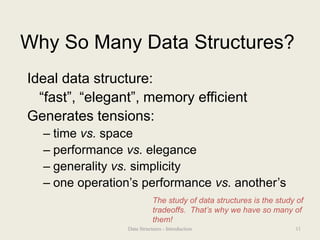
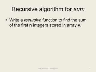
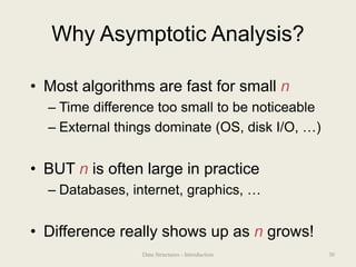
This document provides an overview of a Data Structures course. The course will cover basic data structures and algorithms used in software development. Students will learn about common data structures like lists, stacks, and queues; analyze the runtime of algorithms; and practice implementing data structures. The goal is for students to understand which data structures are appropriate for different problems and be able to justify design decisions. Key concepts covered include abstract data types, asymptotic analysis to evaluate algorithms, and the tradeoffs involved in choosing different data structure implementations.

1. CSE 326: Data Structures
Introduction
1
Data Structures - Introduction

2. Class Overview
• Introduction to many of the basic data structures
used in computer software
– Understand the data structures
– Analyze the algorithms that use them
– Know when to apply them
• Practice design and analysis of data structures.
• Practice using these data structures by writing
programs.
• Make the transformation from programmer to
computer scientist
2
Data Structures - Introduction

3. Goals
• You will understand
– what the tools are for storing and processing common
data types
– which tools are appropriate for which need
• So that you can
– make good design choices as a developer, project
manager, or system customer
• You will be able to
– Justify your design decisions via formal reasoning
– Communicate ideas about programs clearly and
precisely
3
Data Structures - Introduction

4. Goals
“I will, in fact, claim that the difference
between a bad programmer and a good
one is whether he considers his code or
his data structures more important. Bad
programmers worry about the code. Good
programmers worry about data structures
and their relationships.”
Linus Torvalds, 2006
4
Data Structures - Introduction

5. Goals
“Show me your flowcharts and conceal
your tables, and I shall continue to be
mystified. Show me your tables, and I
won’t usually need your flowcharts; they’ll
be obvious.”
Fred Brooks, 1975
5
Data Structures - Introduction

6. Data Structures
“Clever” ways to organize information in
order to enable efficient computation
– What do we mean by clever?
– What do we mean by efficient?
6
Data Structures - Introduction

7. Picking the best
Data Structure for the job
• The data structure you pick needs to
support the operations you need
• Ideally it supports the operations you will
use most often in an efficient manner
• Examples of operations:
– A List with operations insert and delete
– A Stack with operations push and pop
7
Data Structures - Introduction

8. Terminology
• Abstract Data Type (ADT)
– Mathematical description of an object with set of
operations on the object. Useful building block.
• Algorithm
– A high level, language independent, description of a
step-by-step process
• Data structure
– A specific family of algorithms for implementing an
abstract data type.
• Implementation of data structure
– A specific implementation in a specific language
8
Data Structures - Introduction

9. Terminology examples
• A stack is an abstract data type supporting
push, pop and isEmpty operations
• A stack data structure could use an array, a
linked list, or anything that can hold data
• One stack implementation is java.util.Stack;
another is java.util.LinkedList
9
Data Structures - Introduction

10. Concepts vs. Mechanisms
• Abstract
• Pseudocode
• Algorithm
– A sequence of high-level,
language independent
operations, which may act
upon an abstracted view of
data.
• Abstract Data Type (ADT)
– A mathematical description
of an object and the set of
operations on the object.
• Concrete
• Specific programming language
• Program
– A sequence of operations in a
specific programming language,
which may act upon real data in
the form of numbers, images,
sound, etc.
• Data structure
– A specific way in which a
program’s data is represented,
which reflects the programmer’s
design choices/goals.
10
Data Structures - Introduction

11. Why So Many Data Structures?
Ideal data structure:
“fast”, “elegant”, memory efficient
Generates tensions:
– time vs. space
– performance vs. elegance
– generality vs. simplicity
– one operation’s performance vs. another’s
The study of data structures is the study of
tradeoffs. That’s why we have so many of
them!
11
Data Structures - Introduction

12. Today’s Outline
• Introductions
• Administrative Info
• What is this course about?
• Review: Queues and stacks
12
Data Structures - Introduction

13. First Example: Queue ADT
• FIFO: First In First Out
• Queue operations
create
destroy
enqueue
dequeue
is_empty
F E D C B
enqueue dequeue
G A
13
Data Structures - Introduction

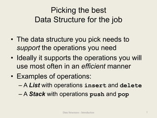
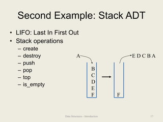
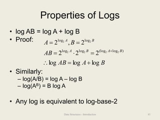
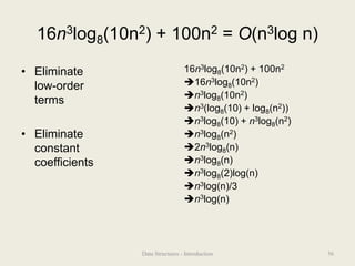
14. Circular Array Queue Data
Structure
enqueue(Object x) {
Q[back] = x ;
back = (back + 1) % size
}
b c d e f
Q
0 size - 1
front back
dequeue() {
x = Q[front] ;
front = (front + 1) % size;
return x ;
}
14
Data Structures - Introduction

15. Linked List Queue Data Structure
b c d e f
front back
void enqueue(Object x) {
if (is_empty())
front = back = new Node(x)
else
back->next = new Node(x)
back = back->next
}
bool is_empty() {
return front == null
}
Object dequeue() {
assert(!is_empty)
return_data = front->data
temp = front
front = front->next
delete temp
return return_data
}
15
Data Structures - Introduction

16. Circular Array vs. Linked List
• Too much space
• Kth element accessed
“easily”
• Not as complex
• Could make array
more robust
• Can grow as needed
• Can keep growing
• No back looping
around to front
• Linked list code more
complex
16
Data Structures - Introduction

17. Second Example: Stack ADT
• LIFO: Last In First Out
• Stack operations
– create
– destroy
– push
– pop
– top
– is_empty
A
B
C
D
E
F
E D C B A
F
17
Data Structures - Introduction

18. Stacks in Practice
• Function call stack
• Removing recursion
• Balancing symbols (parentheses)
• Evaluating Reverse Polish Notation
18
Data Structures - Introduction

19. Data Structures
Asymptotic Analysis
19
Data Structures - Introduction

20. Algorithm Analysis: Why?
• Correctness:
– Does the algorithm do what is intended.
• Performance:
– What is the running time of the algorithm.
– How much storage does it consume.
• Different algorithms may be correct
– Which should I use?
20
Data Structures - Introduction

21. Recursive algorithm for sum
• Write a recursive function to find the sum
of the first n integers stored in array v.
21
Data Structures - Introduction

22. Proof by Induction
• Basis Step: The algorithm is correct for a base
case or two by inspection.
• Inductive Hypothesis (n=k): Assume that the
algorithm works correctly for the first k cases.
• Inductive Step (n=k+1): Given the hypothesis
above, show that the k+1 case will be calculated
correctly.
22
Data Structures - Introduction

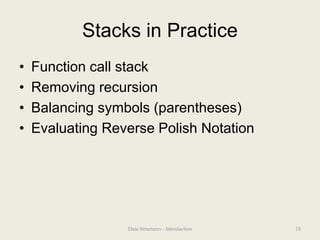
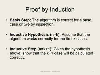
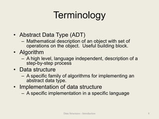
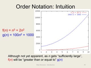
23. Program Correctness by Induction
• Basis Step:
sum(v,0) = 0. 
• Inductive Hypothesis (n=k):
Assume sum(v,k) correctly returns sum of first k
elements of v, i.e. v[0]+v[1]+…+v[k-1]+v[k]
• Inductive Step (n=k+1):
sum(v,n) returns
v[k]+sum(v,k-1)= (by inductive hyp.)
v[k]+(v[0]+v[1]+…+v[k-1])=
v[0]+v[1]+…+v[k-1]+v[k] 
23
Data Structures - Introduction

24. Algorithms vs Programs
• Proving correctness of an algorithm is very important
– a well designed algorithm is guaranteed to work correctly and its
performance can be estimated
• Proving correctness of a program (an implementation) is
fraught with weird bugs
– Abstract Data Types are a way to bridge the gap between
mathematical algorithms and programs
24
Data Structures - Introduction

25. Comparing Two Algorithms
GOAL: Sort a list of names
“I’ll buy a faster CPU”
“I’ll use C++ instead of Java – wicked fast!”
“Ooh look, the –O4 flag!”
“Who cares how I do it, I’ll add more memory!”
“Can’t I just get the data pre-sorted??”
25
Data Structures - Introduction

26. Comparing Two Algorithms
• What we want:
– Rough Estimate
– Ignores Details
• Really, independent of details
– Coding tricks, CPU speed, compiler
optimizations, …
– These would help any algorithms equally
– Don’t just care about running time – not a good
enough measure
26
Data Structures - Introduction

27. Big-O Analysis
• Ignores “details”
• What details?
– CPU speed
– Programming language used
– Amount of memory
– Compiler
– Order of input
– Size of input … sorta.
27
Data Structures - Introduction

28. Analysis of Algorithms
• Efficiency measure
– how long the program runs time complexity
– how much memory it uses space complexity
• Why analyze at all?
– Decide what algorithm to implement before
actually doing it
– Given code, get a sense for where bottlenecks
must be, without actually measuring it
28
Data Structures - Introduction

29. Asymptotic Analysis
• Complexity as a function of input size n
T(n) = 4n + 5
T(n) = 0.5 n log n - 2n + 7
T(n) = 2n + n3 + 3n
• What happens as n grows?
29
Data Structures - Introduction

30. Why Asymptotic Analysis?
• Most algorithms are fast for small n
– Time difference too small to be noticeable
– External things dominate (OS, disk I/O, …)
• BUT n is often large in practice
– Databases, internet, graphics, …
• Difference really shows up as n grows!
30
Data Structures - Introduction

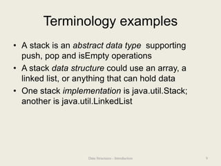
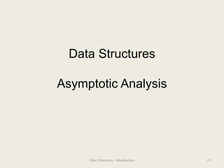
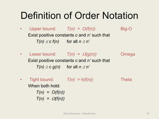
31. Exercise - Searching
bool ArrayFind(int array[], int n, int key){
// Insert your algorithm here
}
2 3 5 16 37 50 73 75 126
What algorithm would you
choose to implement this code
snippet?
31
Data Structures - Introduction

32. Analyzing Code
Basic Java operations
Consecutive statements
Conditionals
Loops
Function calls
Recursive functions
Constant time
Sum of times
Larger branch plus test
Sum of iterations
Cost of function body
Solve recurrence relation
32
Data Structures - Introduction

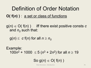
33. Linear Search Analysis
bool LinearArrayFind(int array[],
int n,
int key ) {
for( int i = 0; i < n; i++ ) {
if( array[i] == key )
// Found it!
return true;
}
return false;
}
Best Case:
Worst Case:
33
Data Structures - Introduction

34. Binary Search Analysis
bool BinArrayFind( int array[], int low,
int high, int key ) {
// The subarray is empty
if( low > high ) return false;
// Search this subarray recursively
int mid = (high + low) / 2;
if( key == array[mid] ) {
return true;
} else if( key < array[mid] ) {
return BinArrayFind( array, low,
mid-1, key );
} else {
return BinArrayFind( array, mid+1,
high, key );
}
Best case:
Worst case:
34
Data Structures - Introduction

35. Solving Recurrence Relations
1. Determine the recurrence relation. What is/are the base
case(s)?
2. “Expand” the original relation to find an equivalent general
expression in terms of the number of expansions.
3. Find a closed-form expression by setting the number of
expansions to a value which reduces the problem to a
base case
35
Data Structures - Introduction

36. Data Structures
Asymptotic Analysis
36
Data Structures - Introduction

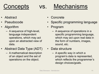
37. Linear Search vs Binary Search
Linear Search Binary Search
Best Case 4 at [0] 4 at [middle]
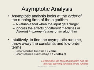
Worst Case 3n+2 4 log n + 4
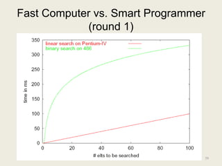
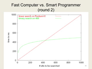
So … which algorithm is better?
What tradeoffs can you make?
37
Data Structures - Introduction

38. Fast Computer vs. Slow
Computer
38

39. Fast Computer vs. Smart Programmer
(round 1)
39

40. Fast Computer vs. Smart Programmer
(round 2)
40

41. Asymptotic Analysis
• Asymptotic analysis looks at the order of
the running time of the algorithm
– A valuable tool when the input gets “large”
– Ignores the effects of different machines or
different implementations of an algorithm
• Intuitively, to find the asymptotic runtime,
throw away the constants and low-order
terms
– Linear search is T(n) = 3n + 2  O(n)
– Binary search is T(n) = 4 log2n + 4  O(log n)
Remember: the fastest algorithm has the
slowest growing function for its runtime
41
Data Structures - Introduction

42. Asymptotic Analysis
• Eliminate low order terms
– 4n + 5 
– 0.5 n log n + 2n + 7 
– n3 + 2n + 3n 
• Eliminate coefficients
– 4n 
– 0.5 n log n 
– n log n2 =>
42
Data Structures - Introduction

43. Properties of Logs
• log AB = log A + log B
• Proof:
• Similarly:
– log(A/B) = log A – log B
– log(AB) = B log A
• Any log is equivalent to log-base-2
B
A
AB
AB
B
A
B
A
B
A
B
A
log
log
log
2
2
2
2
,
2
)
log
(log
log
log
log
log
2
2
2
2
2
2









43
Data Structures - Introduction

44. Order Notation: Intuition
Although not yet apparent, as n gets “sufficiently large”,
f(n) will be “greater than or equal to” g(n)
f(n) = n3 + 2n2
g(n) = 100n2 + 1000
44
Data Structures - Introduction

45. Definition of Order Notation
• Upper bound: T(n) = O(f(n)) Big-O
Exist positive constants c and n’ such that
T(n)  c f(n) for all n  n’
• Lower bound: T(n) = (g(n)) Omega
Exist positive constants c and n’ such that
T(n)  c g(n) for all n  n’
• Tight bound: T(n) = (f(n)) Theta
When both hold:
T(n) = O(f(n))
T(n) = (f(n))
45
Data Structures - Introduction

46. Definition of Order Notation
O( f(n) ) : a set or class of functions
g(n)  O( f(n) ) iff there exist positive consts c
and n0 such that:
g(n)  c f(n) for all n  n0
Example:
100n2 + 1000  5 (n3 + 2n2) for all n  19
So g(n)  O( f(n) )
46
Data Structures - Introduction

47. Order Notation: Example
100n2 + 1000  5 (n3 + 2n2) for all n  19
So f(n)  O( g(n) )
47
Data Structures - Introduction

48. Some Notes on Notation
• Sometimes you’ll see
g(n) = O( f(n) )
• This is equivalent to
g(n)  O( f(n) )
• What about the reverse?
O( f(n) ) = g(n)
48
Data Structures - Introduction

49. Big-O: Common Names
– constant: O(1)
– logarithmic: O(log n) (logkn, log n2  O(log n))
– linear: O(n)
– log-linear: O(n log n)
– quadratic: O(n2)
– cubic: O(n3)
– polynomial: O(nk) (k is a constant)
– exponential: O(cn) (c is a constant > 1)
49
Data Structures - Introduction

50. Meet the Family
• O( f(n) ) is the set of all functions asymptotically less
than or equal to f(n)
– o( f(n) ) is the set of all functions
asymptotically strictly less than f(n)
• ( f(n) ) is the set of all functions asymptotically
greater than or equal to f(n)
– ( f(n) ) is the set of all functions
asymptotically strictly greater than f(n)
• ( f(n) ) is the set of all functions asymptotically equal
to f(n)
50
Data Structures - Introduction

51. Meet the Family, Formally
• g(n)  O( f(n) ) iff
There exist c and n0 such that g(n)  c f(n) for all n  n0
– g(n)  o( f(n) ) iff
There exists a n0 such that g(n) < c f(n) for all c and n  n0
• g(n)  ( f(n) ) iff
There exist c and n0 such that g(n)  c f(n) for all n  n0
– g(n)  ( f(n) ) iff
There exists a n0 such that g(n) > c f(n) for all c and n  n0
• g(n)  ( f(n) ) iff
g(n)  O( f(n) ) and g(n)  ( f(n) )
Equivalent to: limn g(n)/f(n) = 0
Equivalent to: limn g(n)/f(n) = 
51
Data Structures - Introduction

52. Big-Omega et al. Intuitively
Asymptotic Notation Mathematics
Relation
O 
 
 =
o <
 >
52
Data Structures - Introduction

53. Pros and Cons
of Asymptotic Analysis
53
Data Structures - Introduction

54. Perspective: Kinds of Analysis
• Running time may depend on actual data
input, not just length of input
• Distinguish
– Worst Case
• Your worst enemy is choosing input
– Best Case
– Average Case
• Assumes some probabilistic distribution of inputs
– Amortized
• Average time over many operations
54
Data Structures - Introduction

55. Types of Analysis
Two orthogonal axes:
– Bound Flavor
• Upper bound (O, o)
• Lower bound (, )
• Asymptotically tight ()
– Analysis Case
• Worst Case (Adversary)
• Average Case
• Best Case
• Amortized 55
Data Structures - Introduction

56. 16n3log8(10n2) + 100n2 = O(n3log n)
• Eliminate
low-order
terms
• Eliminate
constant
coefficients
16n3log8(10n2) + 100n2
16n3log8(10n2)
n3log8(10n2)
n3(log8(10) + log8(n2))
n3log8(10) + n3log8(n2)
n3log8(n2)
2n3log8(n)
n3log8(n)
n3log8(2)log(n)
n3log(n)/3
n3log(n)
56
Data Structures - Introduction