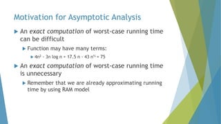
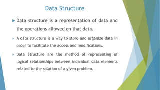
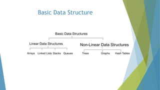
This document outlines a course on programming and data structures in C. It discusses key concepts like abstract data types, asymptotic analysis, various data structures like arrays, stacks, queues, linked lists, trees, and graphs. It covers different algorithms for searching, sorting and indexing of data. The objectives are to learn a program-independent view of data structures and their usage in algorithms. Various data structures, their representations and associated operations are explained. Methods for analyzing algorithms to determine their time and space complexity are also presented.

1. PROGRAMMING AND
DATA STRUCTURES IN C
Ms. UMA. S
Assistant Professor
Computer Science/Computer Applications
Thiruvalluvar University College of Arts and Science, Tirupattur

2. OBJECTIVES
 Learning program independent view of data structures,
including its representation and operations performed on
them, which are then linked to sorting, searching and
indexing methods to increase the knowledge of usage of
data structures in algorithmic perspective.

3.  UNIT-I
 Abstract Data Types –
 Asymptotic Notations: Big-Oh, Omega and Theta –
 Best, Worst and Average case Analysis: Definition and an example –
 Arrays and its representations –
 Stacks and Queues –
 Linked lists –
 Linked list based implementation of Stacks and Queues –
 Evaluation of Expressions –
 Linked list based polynomial addition.

4.  UNIT-II
 Trees –
 Binary Trees – Binary tree representation and traversals –
 Threaded binary trees –
 Binary tree representation of trees –
 Application of trees: Set representation and Union-
 Find operations –
 Graph and its representations –
 Graph Traversals –
 Connected components

5.  UNIT-III
 AVL Trees – Red-Black Trees – Splay Trees – Binary Heap – Leftist Heap
UNIT–IV
 Insertion sort – Merge sort – Quick sort – Heap sort – Sorting with disks – k-
way merging – Sorting with tapes – Polyphase merge.
 UNIT-V
 Linear Search – Binary Search - Hash tables – Overflow handling – Cylinder
Surface Indexing – Hash Index – B-Tree Indexing.

6.  TEXT BOOK
 1. Ellis Horowitz and Sartaj Sahni, Fundamentals of Data Structures, Galgotia
Book Sorce, Gurgaon, 1993.
 2. Gregory L. Heilman, Data Structures, Algorithms and Object Oriented
Programming, Tata Mcgraw-Hill, New Delhi, 2002.
 REFERENCES
 1. Jean-Paul Tremblay and Paul G. Sorenson, An Introduction to Data
Structures with Applications, Second Edition, Tata McGraw-Hill, New Delhi,
1991.
 2. Alfred V. Aho, John E. Hopcroft and Jeffry D. Ullman, Data Structures and
Algorithms, Pearson Education, New Delhi, 2006

7. Data Structure
 Data structure is a representation of data and
the operations allowed on that data.
 A data structure is a way to store and organize data in
order to facilitate the access and modifications.
 Data Structure are the method of representing of
logical relationships between individual data elements
related to the solution of a given problem.

8. Basic Data Structure
Basic Data Structures
Linear Data Structures Non-Linear Data Structures
Arrays Linked Lists Stacks Queues Trees Graphs Hash Tables

9. array
Linked list
tree
queue
stack

10. Selection of Data Structure
 The choice of particular data model depends on
two consideration:
It must be rich enough in structure to represent
the relationship between data elements
The structure should be simple enough that one
can effectively process the data when
necessary

11. Types of Data Structure
Linear: In Linear data structure, values
are arrange in linear fashion.
 Array: Fixed-size
 Linked-list: Variable-size
 Stack: Add to top and remove from top
 Queue: Add to back and remove from front
 Priority queue: Add anywhere, remove the highest priority

12. Types of Data Structure
 Non-Linear: The data values in this structure
are not arranged in order.
 Hash tables: Unordered lists which use a ‘hash
function’ to insert and search
 Tree: Data is organized in branches.
 Graph: A more general branching structure, with
less strict connection conditions than for a tree

13. Type of Data Structures
 Homogenous: In this type of data structures,
values of the same types of data are stored.
 Array
 Non-Homogenous: In this type of data structures,
data values of different types are grouped and
stored.
 Structures
 Classes

14. Abstract Data Type and Data Structure
 Definition:-
 Abstract Data Types (ADTs) stores data and allow
various operations on the data to access and change
it.
 A mathematical model, together with various
operations defined on the model
 An ADT is a collection of data and associated
operations for manipulating that data

15.  Data Structures
 Physical implementation of an ADT
 data structures used in implementations are provided
in a language (primitive or built-in) or are built from the
language constructs (user-defined)
 Each operation associated with the ADT is implemented
by one or more subroutines in the implementation

16. Abstract Data Type
 ADTs support abstraction, encapsulation, and
information hiding.
 Abstraction is the structuring of a problem into well-
defined entities by defining their data and
operations.
 The principle of hiding the used data structure and to
only provide a well-defined interface is known as
encapsulation.

17. Core Operations of ADT
 Every Collection ADT should provide a way to:
 add an item
 remove an item
 find, retrieve, or access an item
 Other possibilities
 is the collection empty
 make the collection empty
 give me a sub set of the collection

18. • No single data structure works well for all purposes, and
so it is important to know the strengths and limitations
of several of them

19. 19
Analyzing Algorithms
 Predict the amount of resources required:
• memory: how much space is needed?
• computational time: how fast the algorithm runs?
 FACT: running time grows with the size of the
input

20.  Input size (number of elements in the input)
 Size of an array, polynomial degree, # of elements in
a matrix, # of bits in the binary representation of the
input, vertices and edges in a graph

21. Def: Running time = the number of primitive
operations (steps) executed before termination
 Arithmetic operations (+, -, *), data movement,
control, decision making (if, while), comparison

22. 22
Algorithm Analysis: Example
 Alg.: MIN (a[1], …, a[n])
m ← a[1];
for i ← 2 to n
if a[i] < m
then m ← a[i];

23.  Running time:
 the number of primitive operations (steps) executed
before termination
T(n) =1 [first step] + (n) [for loop] + (n-1) [if
condition] +
(n-1) [the assignment in then] = 3n - 1

24.  Order (rate) of growth:
The leading term of the formula
Expresses the asymptotic behavior of the
algorithm

25. 25
Typical Running Time Functions
 1 (constant running time):
 Instructions are executed once or a few times
 logN (logarithmic)
 A big problem is solved by cutting the original problem in smaller
sizes, by a constant fraction at each step
 N (linear)
 A small amount of processing is done on each input element
 N logN
 A problem is solved by dividing it into smaller problems, solving them
independently and combining the solution

26. 26
Typical Running Time Functions
 N2 (quadratic)
 Typical for algorithms that process all pairs of data items (double
nested loops)
 N3 (cubic)
 Processing of triples of data (triple nested loops)
 NK (polynomial)
 2N (exponential)
 Few exponential algorithms are appropriate for practical use

27. 27
Growth of Functions

28. Complexity Graphs
log(n)
n

29. Complexity Graphs
log(n)
n
n
n log(n)

30. Complexity Graphs
n10
n log(n)
n3
n2

31. Complexity Graphs (log scale)
n10
n20
nn
1.1n
2n
3n

32. Algorithm Complexity
 Worst Case Complexity:
 the function defined by the maximum number of steps taken
on any instance of size n
 Best Case Complexity:
 the function defined by the minimum number of steps taken
on any instance of size n
 Average Case Complexity:
 the function defined by the average number of steps taken
on any instance of size n

33. Best, Worst, and Average Case Complexity
Worst Case
Complexity
Average Case
Complexity
Best Case
Complexity
Number
of steps
N
(input size)

34. Doing the Analysis
It’s hard to estimate the running time
exactly
Best case depends on the input
Average case is difficult to compute
So we usually focus on worst case analysis
Easier to compute
Usually close to the actual running time

35. Strategy: find a function (an equation)
that, for large n, is an upper bound to
the actual function (actual number of
steps, memory usage, etc.)

36. Upper bound
Lower bound
Actual function

37. Motivation for Asymptotic Analysis
 An exact computation of worst-case running time
can be difficult
 Function may have many terms:
 4n2 - 3n log n + 17.5 n - 43 n⅔ + 75
 An exact computation of worst-case running time
is unnecessary
 Remember that we are already approximating running
time by using RAM model