Analysis of data structure asymptotic notations and amortized complexity

1. Data Structures & Algorithms
By Mr. Wubie A. (M.Tech) Dep’t of IT
Mizan-Tepi University
School of Computing
and Informatics

2. Please bring to class
each day
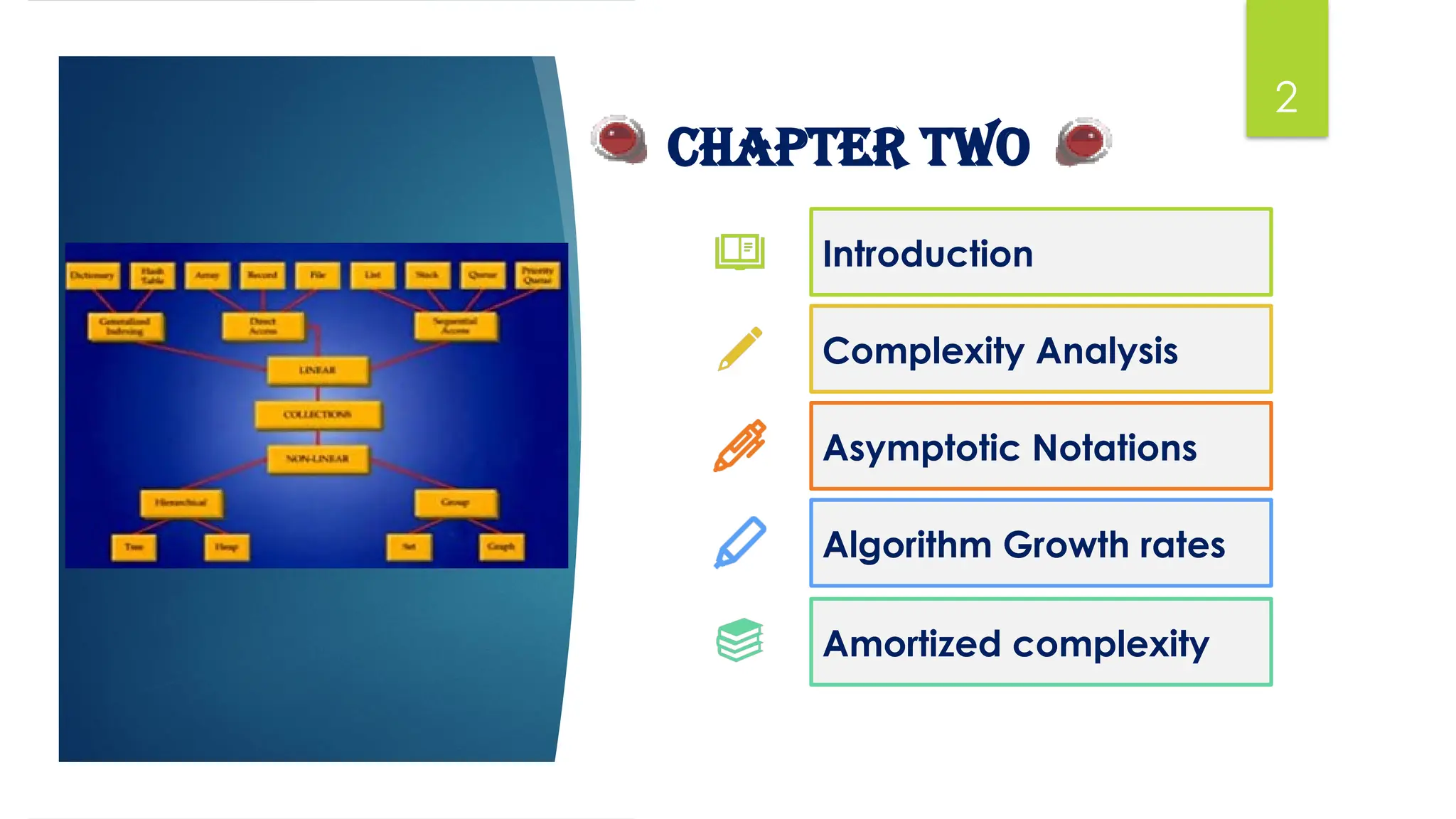
Introduction
Complexity Analysis
Asymptotic Notations
Algorithm Growth rates
Amortized complexity
2
Chapter TWO

3. Introduction
By Mr. Wubie A. (M.Tech)
3
Data structures:
Data
 Data is a collection of facts, numbers, letters or symbols that the computer process
into meaningful information.
Data structure
 A data structure is a way to store and organize data in order to facilitate access and
modifications.
 No single data structure works well for all purposes, and so it is important to know the
strengths and limitations of several of them.
 Data structure is a specialized format for organizing and storing data in memory that
considers not only the elements stored but also their relationship to each other.

4. Introduction
By Mr Wubie A. (M.Tech)
4
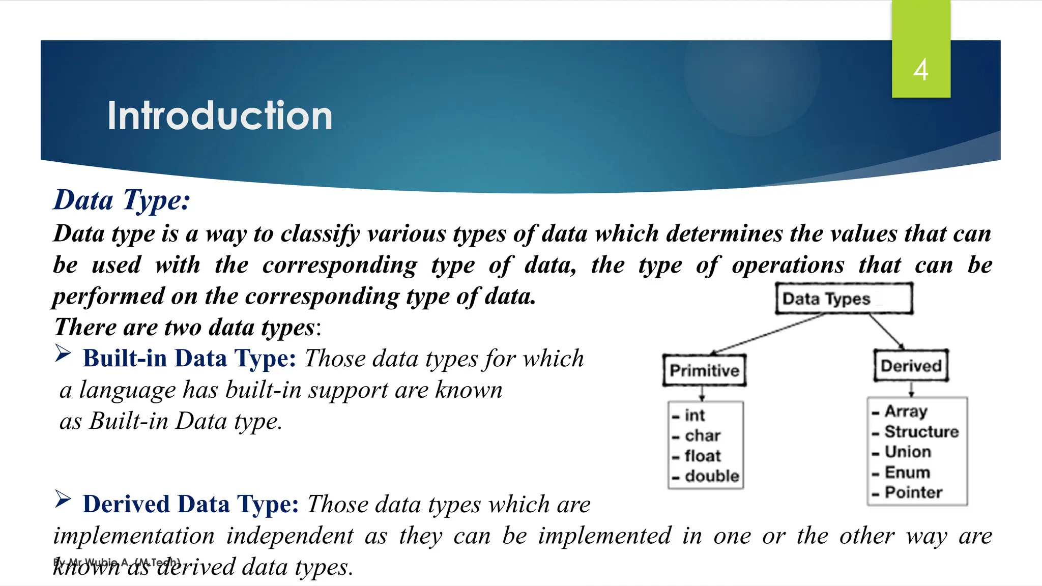
Data Type:
Data type is a way to classify various types of data which determines the values that can
be used with the corresponding type of data, the type of operations that can be
performed on the corresponding type of data.
There are two data types:
 Built-in Data Type: Those data types for which
a language has built-in support are known
as Built-in Data type.
 Derived Data Type: Those data types which are
implementation independent as they can be implemented in one or the other way are
known as derived data types.

5. Introduction
By Mr Wubie A. (M.Tech)
5
Why to Learn Data Structure:
As applications are getting complex and data rich, there are three common problems
that applications face now-a-days
 Data Search − Consider an inventory of 1 million(106) items of a store. If the
application is to search an item, it has to search an item in 1 million(106) items every
time slowing down the search. As data grows, search will become slower.
 Processor speed − Processor speed although being very high, falls limited if the data
grows to billion records.
 Multiple requests − As thousands of users can search data simultaneously on a web
server, even the fast server fails while searching the data..

6. Introduction
By Mr Wubie A. (M.Tech)
6
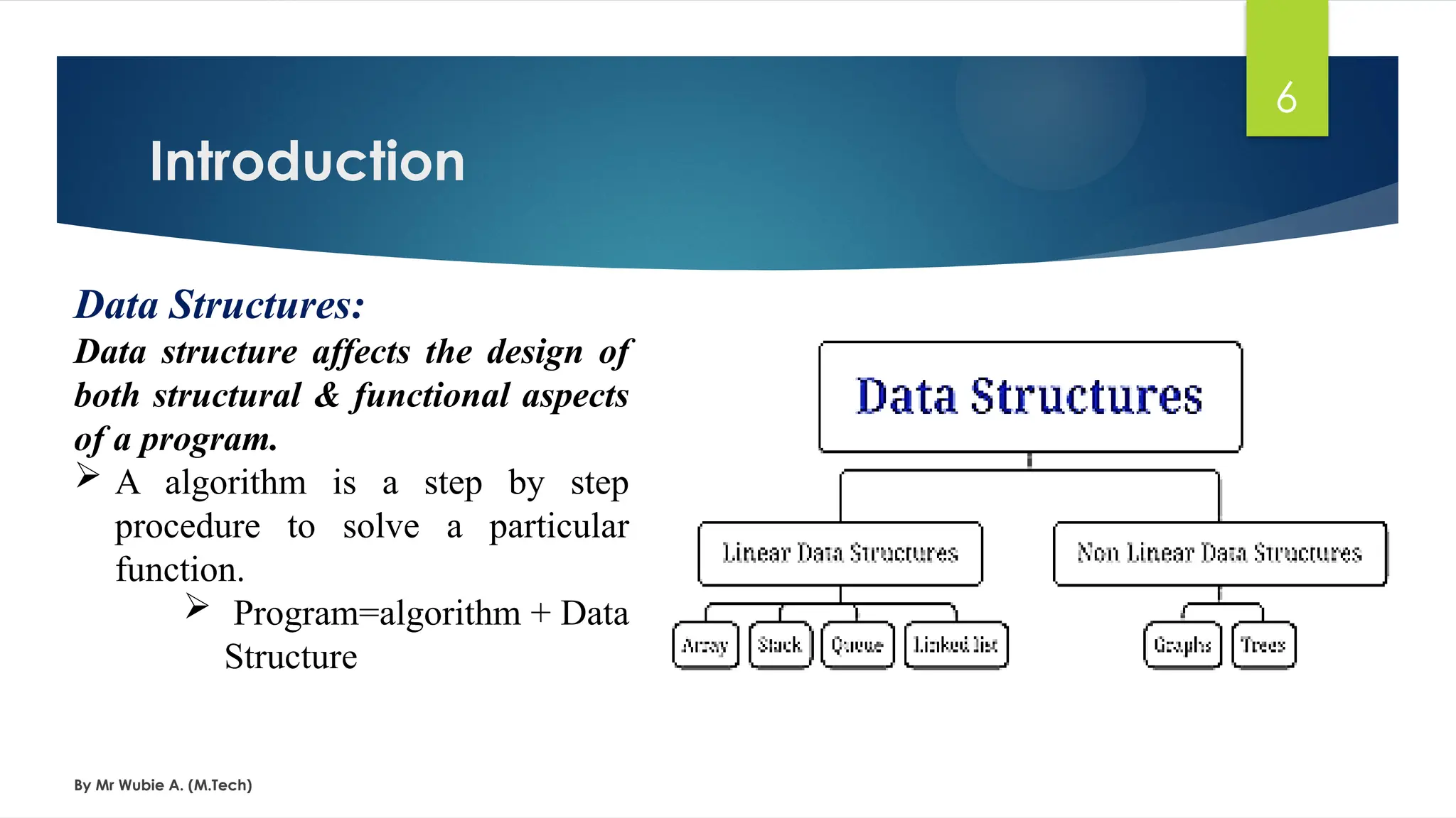
Data Structures:
Data structure affects the design of
both structural & functional aspects
of a program.
 A algorithm is a step by step
procedure to solve a particular
function.
 Program=algorithm + Data
Structure

7. Introduction
By Mr Wubie A. (M.Tech)
7
Classification of Data Structure:

8. Introduction
By Mr Wubie A. (M.Tech)
8
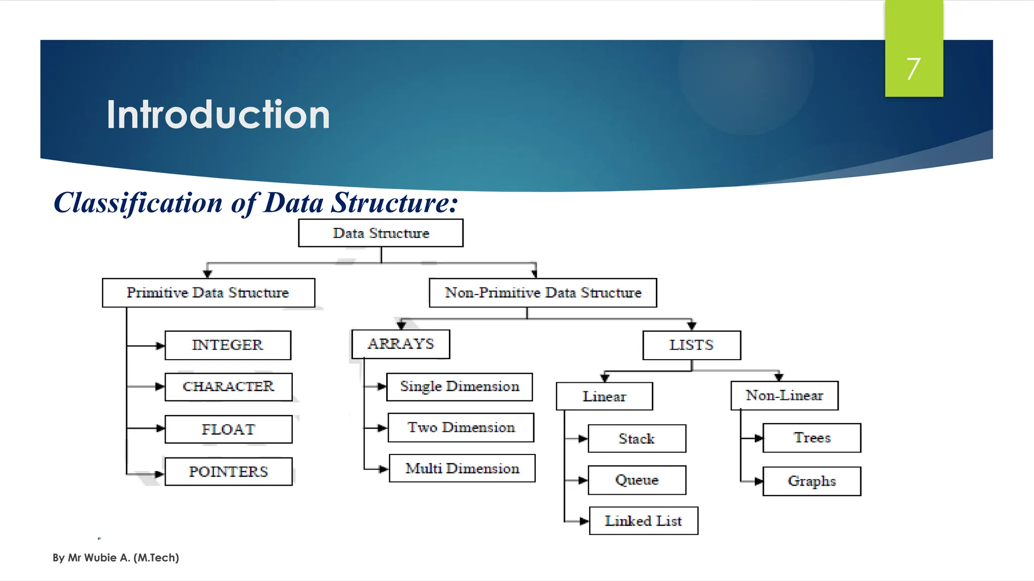
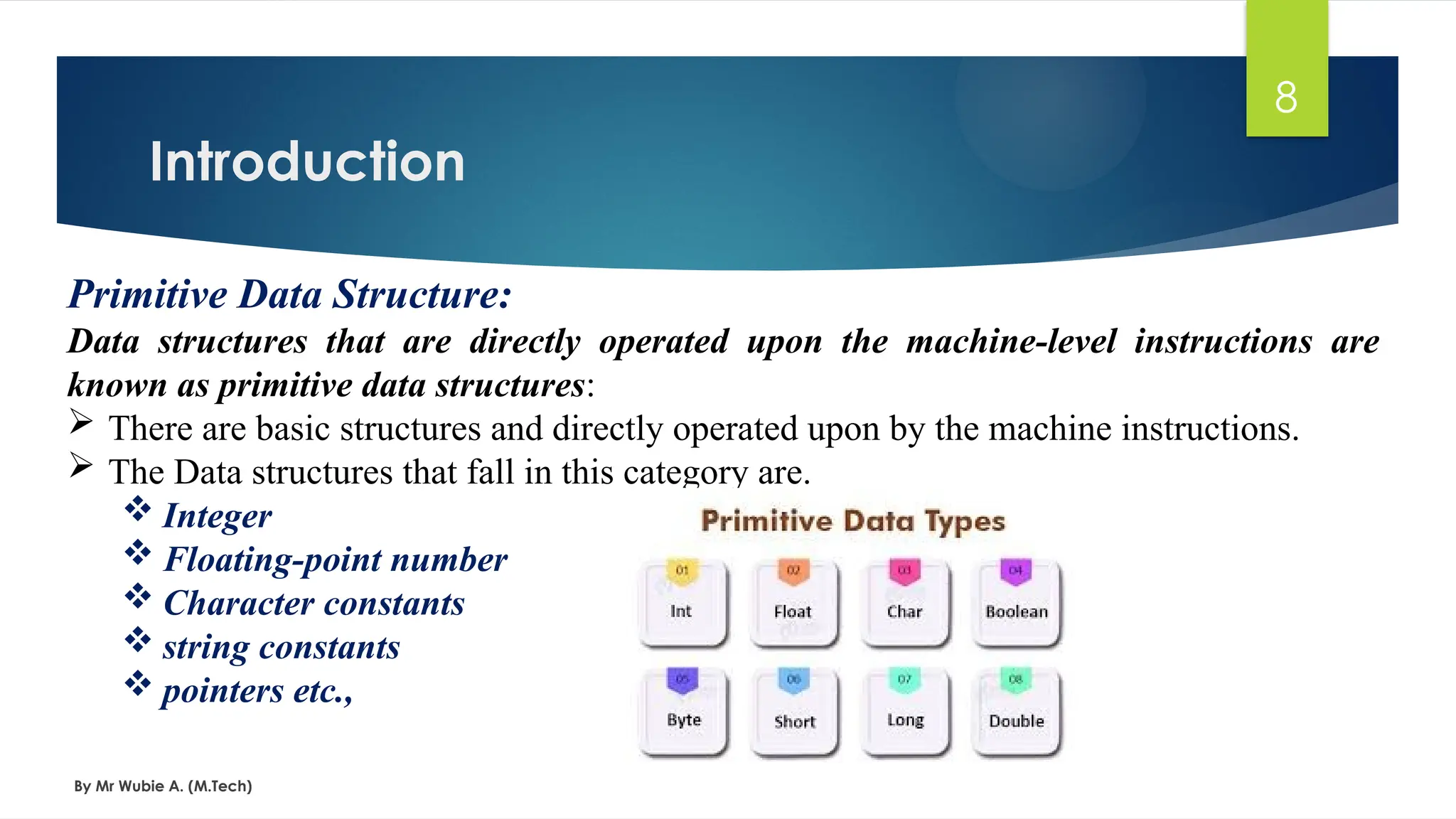
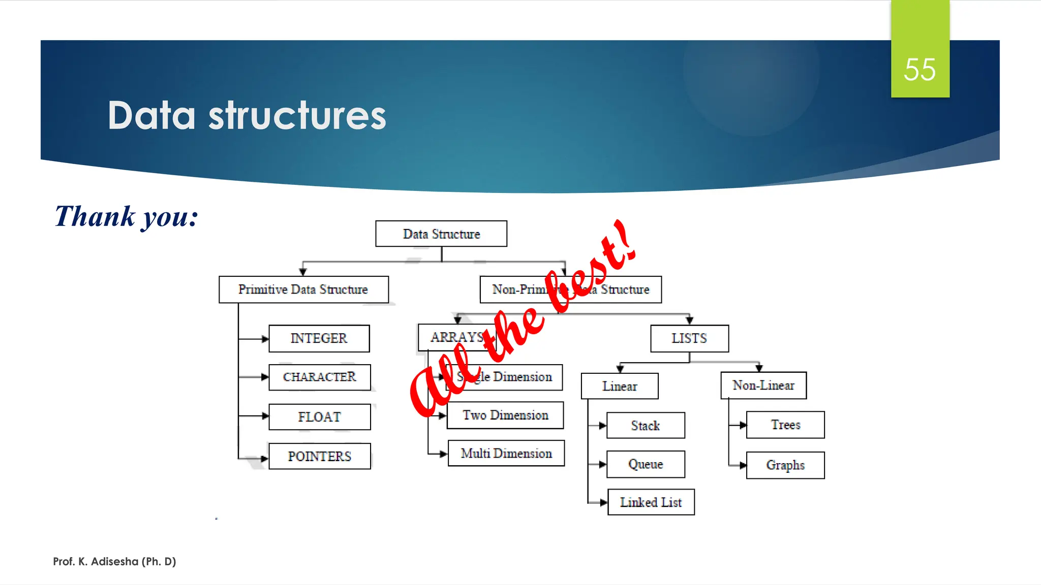
Primitive Data Structure:
Data structures that are directly operated upon the machine-level instructions are
known as primitive data structures:
 There are basic structures and directly operated upon by the machine instructions.
 The Data structures that fall in this category are.
 Integer
 Floating-point number
 Character constants
 string constants
 pointers etc.,

9. Introduction
By Mr Wubie A. (M.Tech)
9
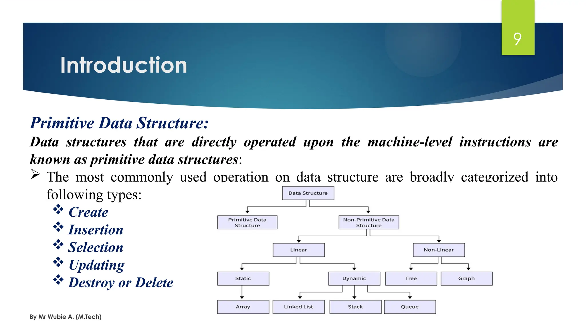
Primitive Data Structure:
Data structures that are directly operated upon the machine-level instructions are
known as primitive data structures:
 The most commonly used operation on data structure are broadly categorized into
following types:
 Create
 Insertion
 Selection
 Updating
 Destroy or Delete

10. Introduction
By Mr Wubie A. (M.Tech)
10
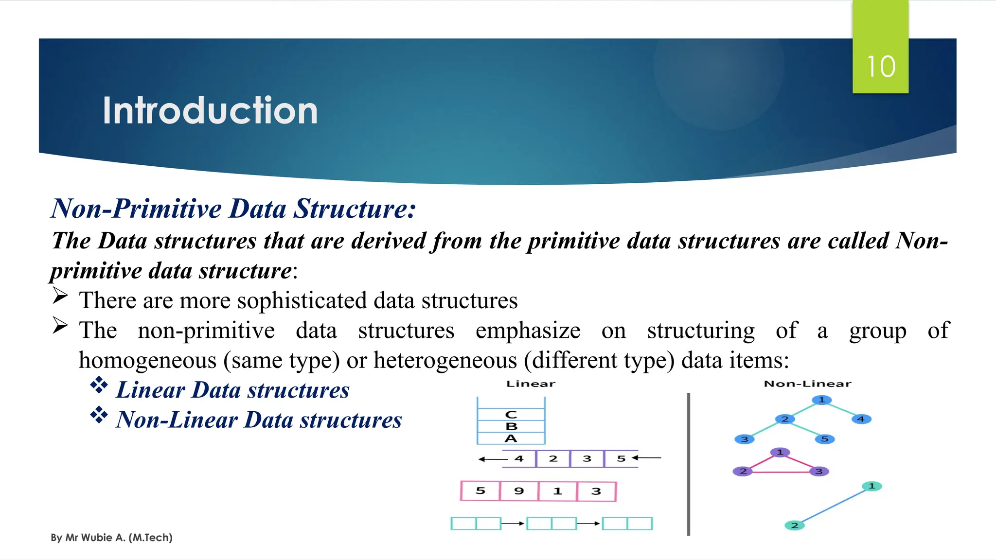
Non-Primitive Data Structure:
The Data structures that are derived from the primitive data structures are called Non-
primitive data structure:
 There are more sophisticated data structures
 The non-primitive data structures emphasize on structuring of a group of
homogeneous (same type) or heterogeneous (different type) data items:
 Linear Data structures
 Non-Linear Data structures

11. Introduction
By Mr Wubie A. (M.Tech)
11
Non-Primitive Data Structure:
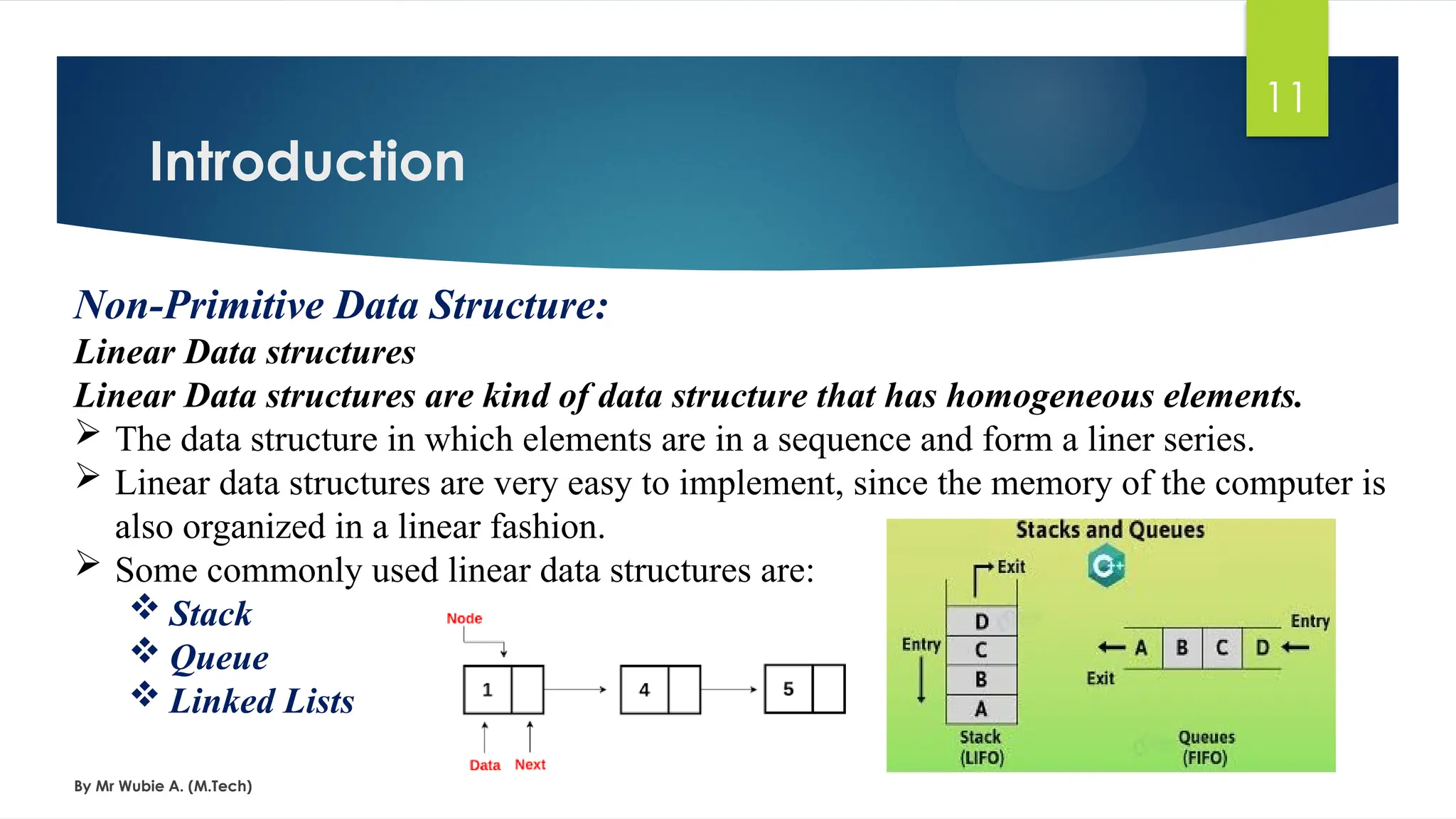
Linear Data structures
Linear Data structures are kind of data structure that has homogeneous elements.
 The data structure in which elements are in a sequence and form a liner series.
 Linear data structures are very easy to implement, since the memory of the computer is
also organized in a linear fashion.
 Some commonly used linear data structures are:
 Stack
 Queue
 Linked Lists

12. Introduction
By Mr Wubie A. (M.Tech)
12
Non-Primitive Data Structure:
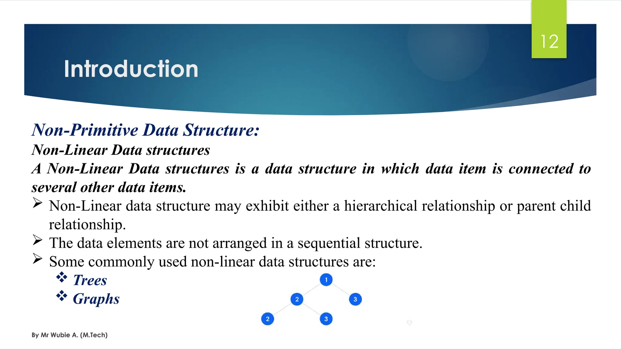
Non-Linear Data structures
A Non-Linear Data structures is a data structure in which data item is connected to
several other data items.
 Non-Linear data structure may exhibit either a hierarchical relationship or parent child
relationship.
 The data elements are not arranged in a sequential structure.
 Some commonly used non-linear data structures are:
 Trees
 Graphs

13. Introduction
By Mr Wubie A. (M.Tech)
13
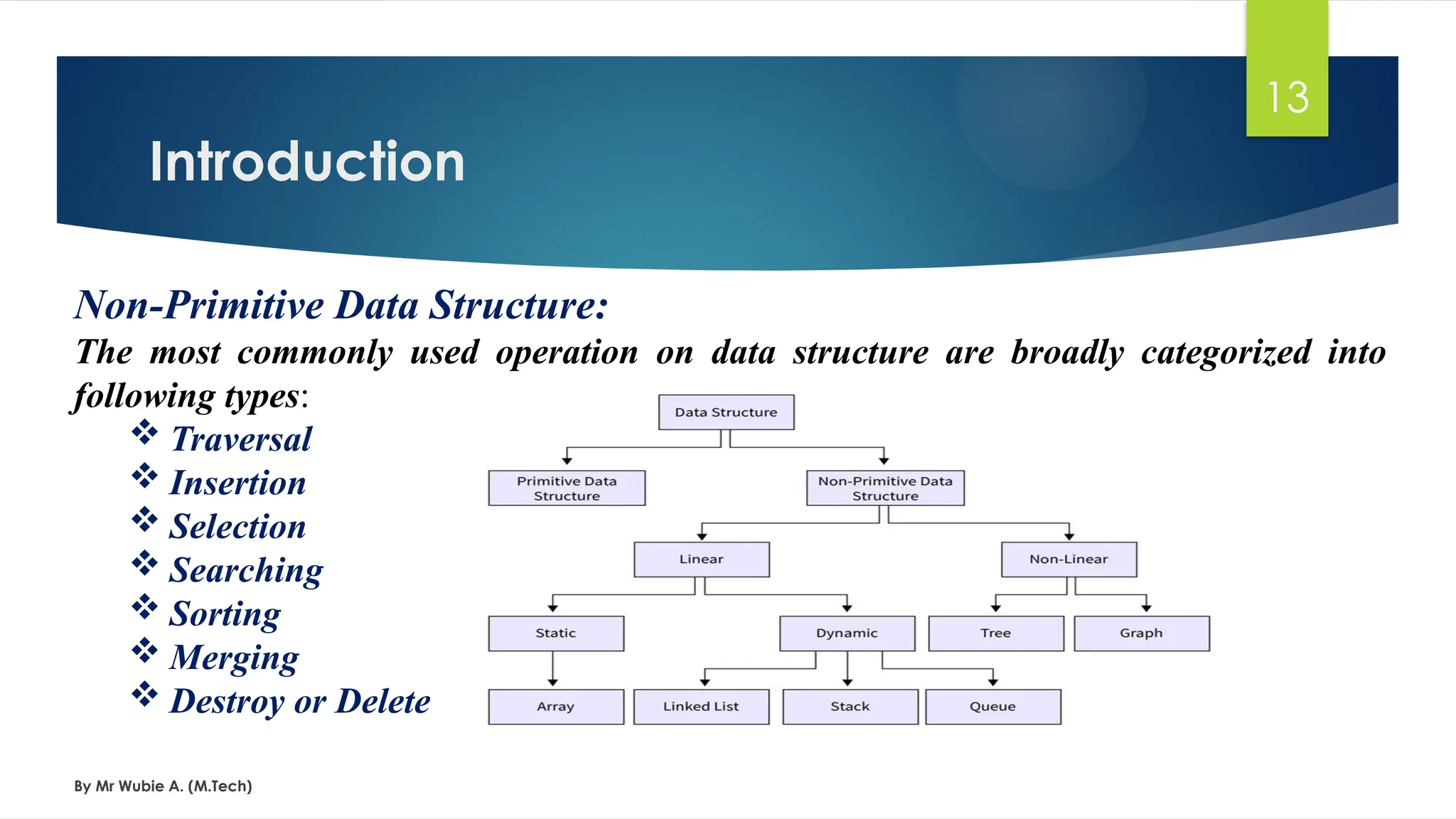
Non-Primitive Data Structure:
The most commonly used operation on data structure are broadly categorized into
following types:
 Traversal
 Insertion
 Selection
 Searching
 Sorting
 Merging
 Destroy or Delete

14. Introduction
By Mr Wubie A. (M.Tech)
14
Differences between Data Structure:
The most commonly used differences between on data structure are broadly categorized
into following types:
 A primitive data structure is generally a basic structure that is usually built into the
language, such as an integer, a float.
 A non-primitive data structure is built out of primitive data structures linked together
in meaningful ways, such as a or a linked-list, binary search tree, AVL Tree, graph etc.

15. Introduction
By Mr Wubie A. (M.Tech)
15
Characteristics of a Data Structure:
Data Structure is a systematic way to organize data in order to use it efficiently.
Following terms are the Characteristics of a data structure.
 Correctness − Data structure implementation should implement its interface correctly.
 Time Complexity − Running time or the execution time of operations of data structure
must be as small as possible.
 Space Complexity − Memory usage of a data structure operation should be as little as
possible.

16. Introduction
By Mr Wubie A. (M.Tech)
16
Abstract data type:
 A type is a collection of values.
 For example, the Boolean type consists of the values true and false.
[Ex: Integer, Boolean, Float]
 A data type is a type together with a collection of operations to manipulate the type.
 For example, an integer variable is a member of the integer data type. Addition
is an example of an operation on the integer data type.
 Solving a problem involves processing data, and an important part of the solution is
the careful organization of the data
 In order to do that, we need to identify:
1. The collection of data items
2. Basic operation that must be performed on them

17. Introduction
By Mr Wubie A. (M.Tech)
17
Abstract data type:
 Abstract Data Type (ADT): a collection of data items together with the operations on
the data . And its implementation is hidden. i.e.
 An ADT does not specify how the data type is implemented. These implementation
details are hidden from the user of the ADT and protected from outside access, a
concept referred to as encapsulation.
 An implementation of ADT consists of storage structures to store the data items and
algorithms for basic operation
 The word “abstract” refers to the fact that the data and the basic operations defined
on it are being studied independently of how they are implemented.
 We think about what can be done with the data, not how it is done.

18. Introduction
By Mr Wubie A. (M.Tech)
18
Algorithms:
Algorithm is a well-defined computational procedure that takes some value or a set of
values as input and produces some value or a set of values as output.. Algorithms are
generally created independent of underlying languages.
 From the data structure point of view, following are some important categories of
algorithms.
 Insert − Algorithm to insert item in a data structure.
 Traverse − Algorithm to visit every item in a data structure.
 Update − Algorithm to update an existing item in a data structure.
 Search − Algorithm to search an item in a data structure.
 Sort − Algorithm to sort items in a certain order.
 Delete − Algorithm to delete an existing item from a data structure.

19. Introduction
By Mr Wubie A. (M.Tech)
19
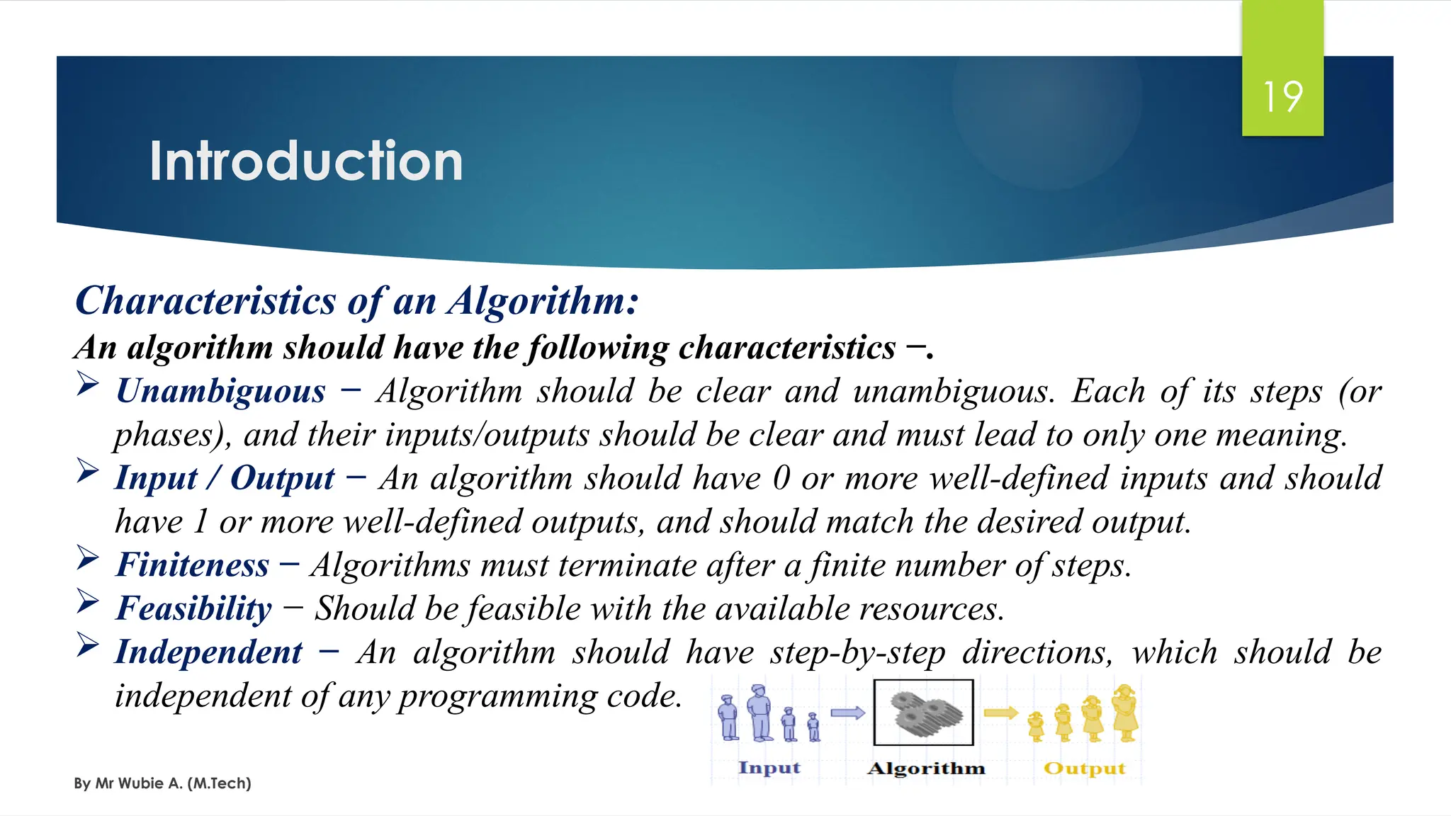
Characteristics of an Algorithm:
An algorithm should have the following characteristics −.
 Unambiguous − Algorithm should be clear and unambiguous. Each of its steps (or
phases), and their inputs/outputs should be clear and must lead to only one meaning.
 Input / Output − An algorithm should have 0 or more well-defined inputs and should
have 1 or more well-defined outputs, and should match the desired output.
 Finiteness − Algorithms must terminate after a finite number of steps.
 Feasibility − Should be feasible with the available resources.
 Independent − An algorithm should have step-by-step directions, which should be
independent of any programming code.

20. Introduction
By Mr Wubie A. (M.Tech)
20
Applications of Data Structure and Algorithms:
How does Google quickly find web pages that contain a search term?
What’s the fastest way to broadcast a message to a network of computers?
 How can a subsequence of DNA be quickly found within the genome?
How does your operating system track which memory (disk or RAM) is
free?

21. Algorithm Analysis:
By Mr Wubie A. (M.Tech)
21
Efficiency of an algorithm can be analyzed at two different stages, before
implementation and after implementation. They are the following .
 A Priori Analysis − This is a theoretical analysis of an algorithm. Efficiency of an
algorithm is measured by assuming factors, like processor speed, are constant and have
no effect on the implementation.
 A Posterior Analysis − This is an empirical analysis of an algorithm. The selected
algorithm is implemented using programming language. In this analysis, actual
statistics like running time and space required, are collected.

22. Algorithm Analysis:
By Mr Wubie A. (M.Tech)
22
 Complexity Analysis is the systematic study of the cost of computation, measured
either in time units or in operations performed, or in the amount of storage space
required.
 The goal is to have a meaningful measure that permits comparison of algorithms
independent of operating platform.
 Space complexity − Space complexity of an algorithm represents the amount of memory
space required by the algorithm in its life cycle..
 Time complexity − Time complexity of an algorithm represents the amount of time
required by the algorithm to run to completion.

23. Algorithm Analysis:
By Mr Wubie A. (M.Tech)
23
Algorithm Performance:
Time
-Instructions take time.
-How fast does the
algorithm perform?
-What affects its runtime?
Space
-Data structures take space
-What kind of data
structures can be used?
-How does choice of data
structure affect the runtime?
We will focus on time:
How to estimate the time required for an algorithm
How to reduce the time required

24. Algorithm Analysis:
By Mr Wubie A. (M.Tech)
24
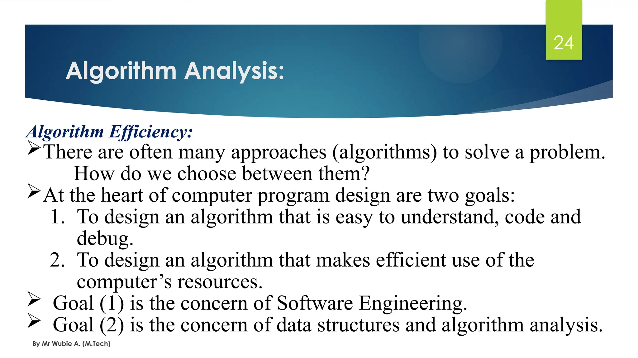
Algorithm Efficiency:
There are often many approaches (algorithms) to solve a problem.
How do we choose between them?
At the heart of computer program design are two goals:
1. To design an algorithm that is easy to understand, code and
debug.
2. To design an algorithm that makes efficient use of the
computer’s resources.
 Goal (1) is the concern of Software Engineering.
 Goal (2) is the concern of data structures and algorithm analysis.

25. Algorithm Analysis:
By Mr Wubie A. (M.Tech)
25
Analysis Rules:
 Algorithm analysis requires a set of rules to determine how operations
are to be counted.
 There is no generally accepted set of rules for algorithm analysis.
 In some cases, an exact count of operations is desired; in other cases, a
general approximation is sufficient.
 The rules presented that follow are typical of those intended to produce
an exact count of operations.

26. Algorithm Analysis:
By Mr Wubie A. (M.Tech)
26
Analysis Rules:
1. We assume an arbitrary time unit.
2. Execution of one of the following operations takes time 1:
-Assignment Operation
-Single Input/Output Operation
-Single Boolean Operations, numeric comparisons
-Single Arithmetic Operations
-Function Return
- array index operations, pointer dereferences
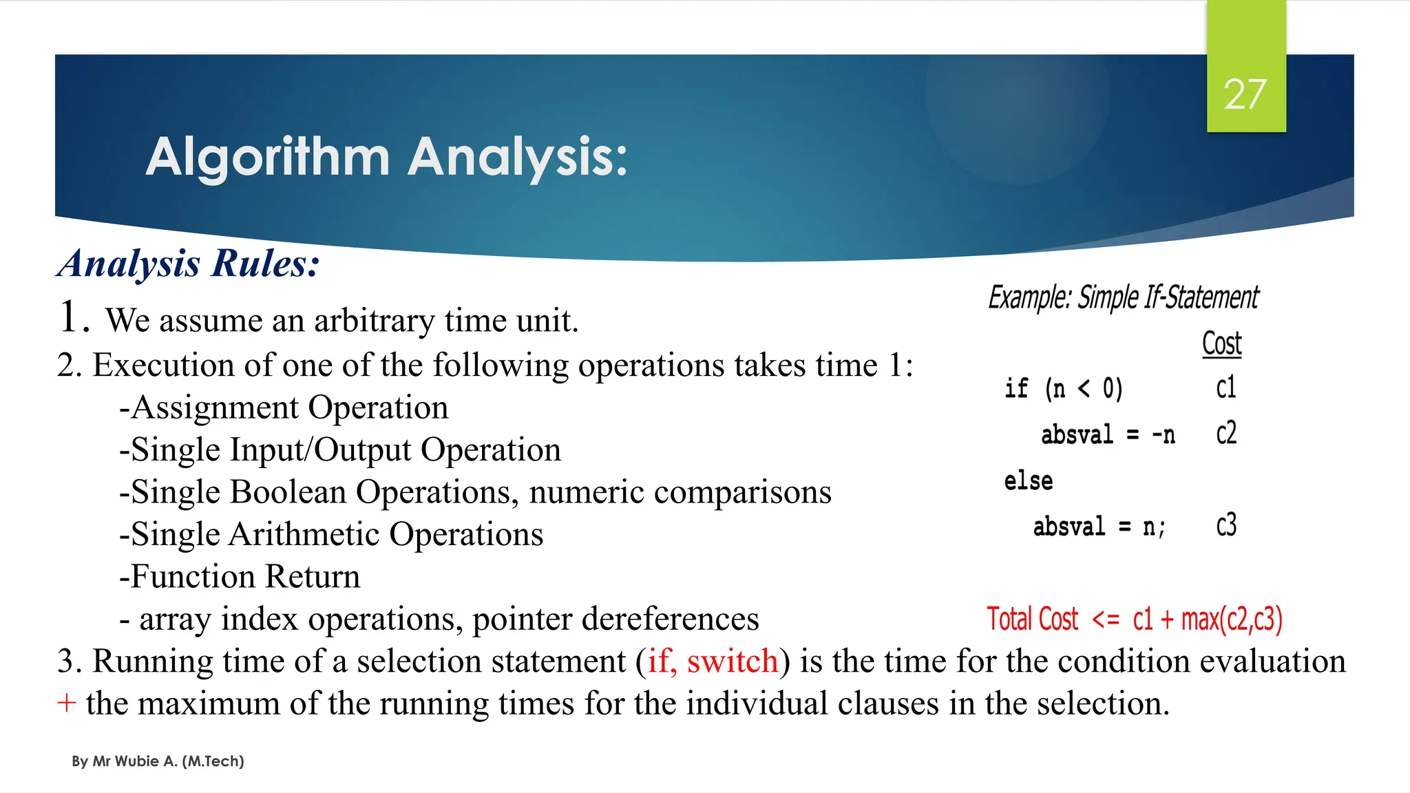
3. Running time of a selection statement (if, switch) is the time for the condition evaluation
+ the maximum of the running times for the individual clauses in the selection.

27. Algorithm Analysis:
By Mr Wubie A. (M.Tech)
27
Analysis Rules:
1. We assume an arbitrary time unit.
2. Execution of one of the following operations takes time 1:
-Assignment Operation
-Single Input/Output Operation
-Single Boolean Operations, numeric comparisons
-Single Arithmetic Operations
-Function Return
- array index operations, pointer dereferences
3. Running time of a selection statement (if, switch) is the time for the condition evaluation
+ the maximum of the running times for the individual clauses in the selection.

28. Algorithm Analysis:
By Mr Wubie A. (M.Tech)
28
Analysis Rules:
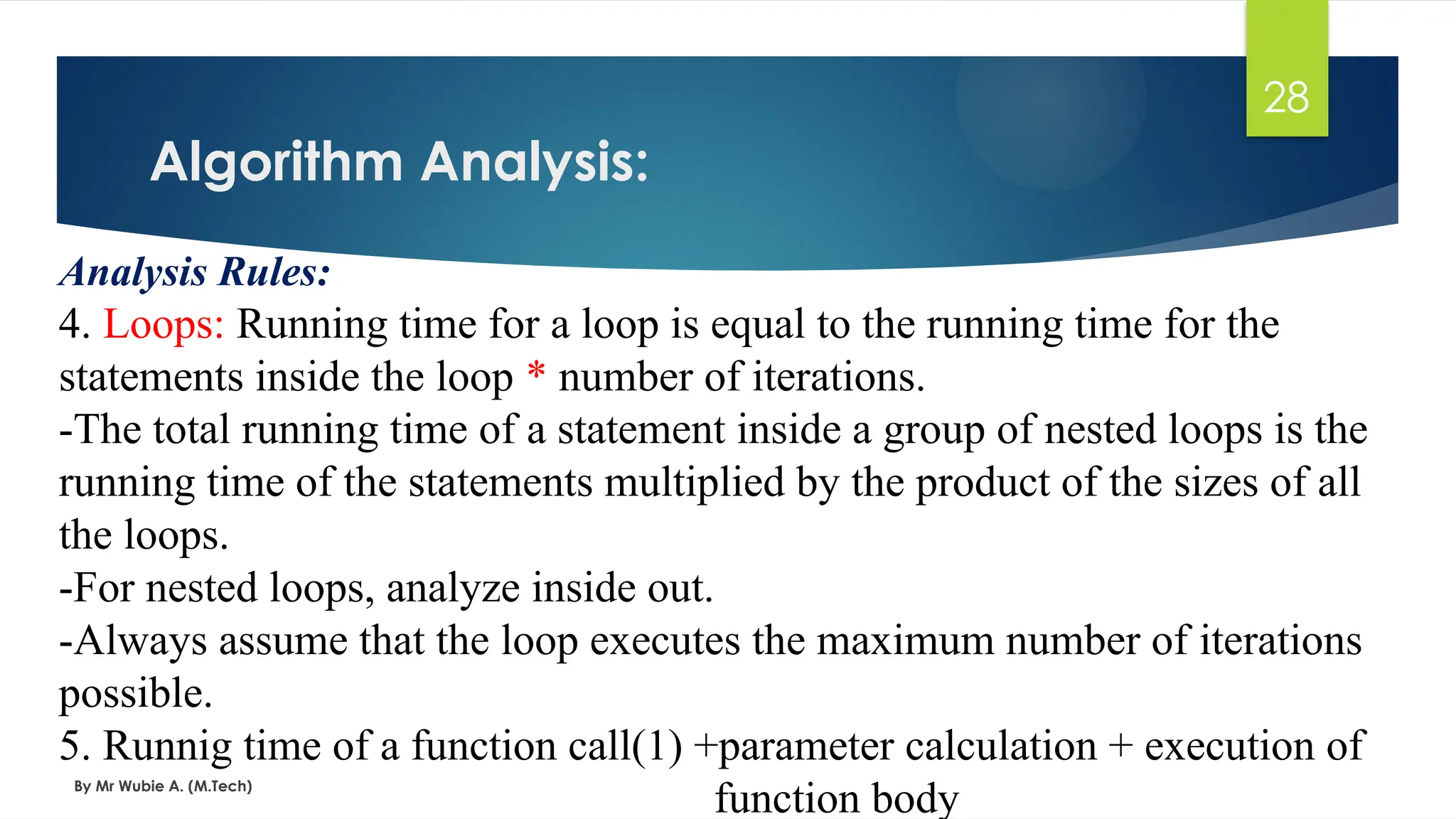
4. Loops: Running time for a loop is equal to the running time for the
statements inside the loop * number of iterations.
-The total running time of a statement inside a group of nested loops is the
running time of the statements multiplied by the product of the sizes of all
the loops.
-For nested loops, analyze inside out.
-Always assume that the loop executes the maximum number of iterations
possible.
5. Runnig time of a function call(1) +parameter calculation + execution of
function body

29. Algorithm Analysis:
By Mr Wubie A. (M.Tech)
29
Analysis Rules:
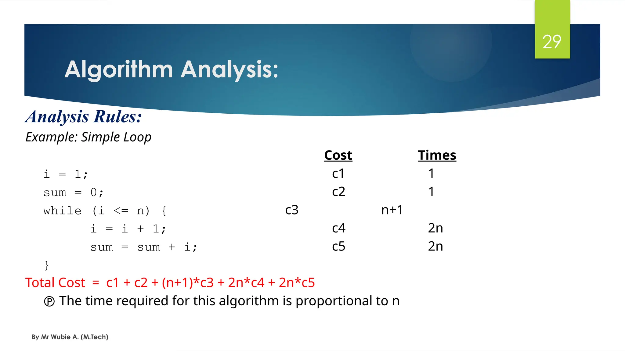
Example: Simple Loop
Cost Times
i = 1; c1 1
sum = 0; c2 1
while (i <= n) { c3 n+1
i = i + 1; c4 2n
sum = sum + i; c5 2n
}
Total Cost = c1 + c2 + (n+1)*c3 + 2n*c4 + 2n*c5
 The time required for this algorithm is proportional to n

30. Algorithm Analysis:
By Mr Wubie A. (M.Tech)
30
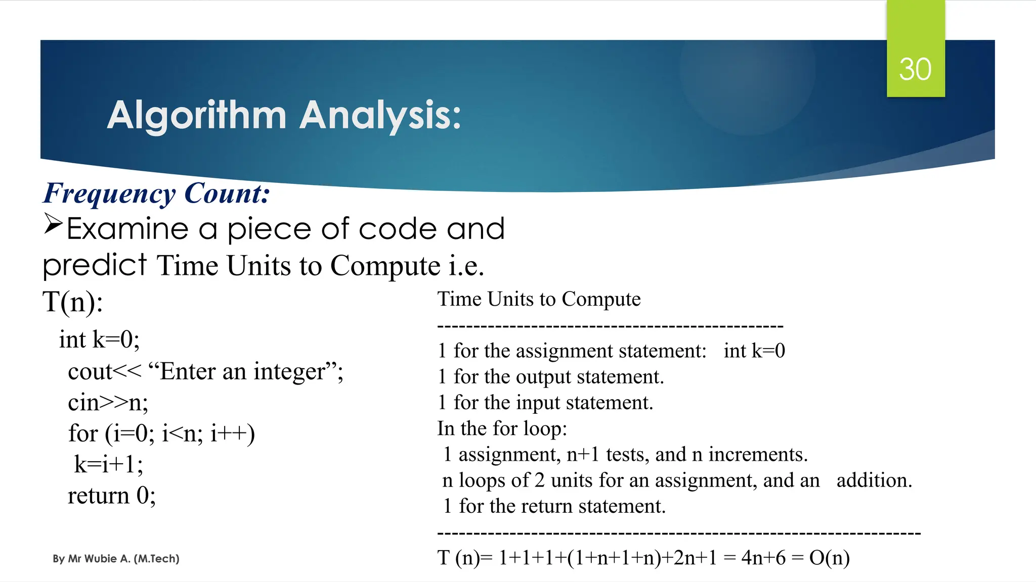
Frequency Count:
Examine a piece of code and
predict Time Units to Compute i.e.
T(n):
int k=0;
cout<< “Enter an integer”;
cin>>n;
for (i=0; i<n; i++)
k=i+1;
return 0;
Time Units to Compute
------------------------------------------------
1 for the assignment statement: int k=0
1 for the output statement.
1 for the input statement.
In the for loop:
1 assignment, n+1 tests, and n increments.
n loops of 2 units for an assignment, and an addition.
1 for the return statement.
-------------------------------------------------------------------
T (n)= 1+1+1+(1+n+1+n)+2n+1 = 4n+6 = O(n)

31. Algorithm Analysis:
By Mr Wubie A. (M.Tech)
31
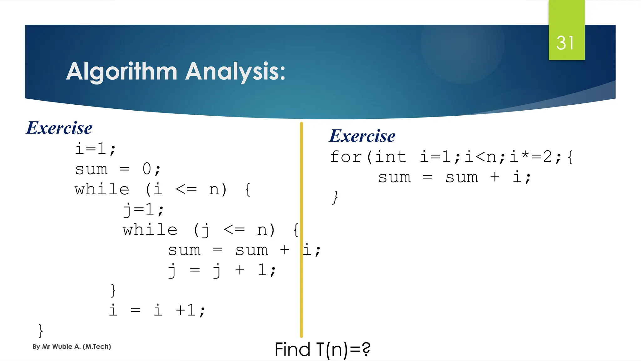
Exercise
i=1;
sum = 0;
while (i <= n) {
j=1;
while (j <= n) {
sum = sum + i;
j = j + 1;
}
i = i +1;
}
Find T(n)=?
Exercise
for(int i=1;i<n;i*=2;{
sum = sum + i;
}

32. Algorithm Analysis:
By Mr Wubie A. (M.Tech)
32
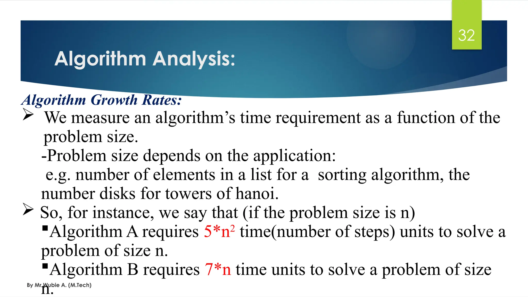
Algorithm Growth Rates:
 We measure an algorithm’s time requirement as a function of the
problem size.
-Problem size depends on the application:
e.g. number of elements in a list for a sorting algorithm, the
number disks for towers of hanoi.
 So, for instance, we say that (if the problem size is n)
Algorithm A requires 5*n2
time(number of steps) units to solve a
problem of size n.
Algorithm B requires 7*n time units to solve a problem of size
n.

33. Algorithm Analysis:
By Mr Wubie A. (M.Tech)
33
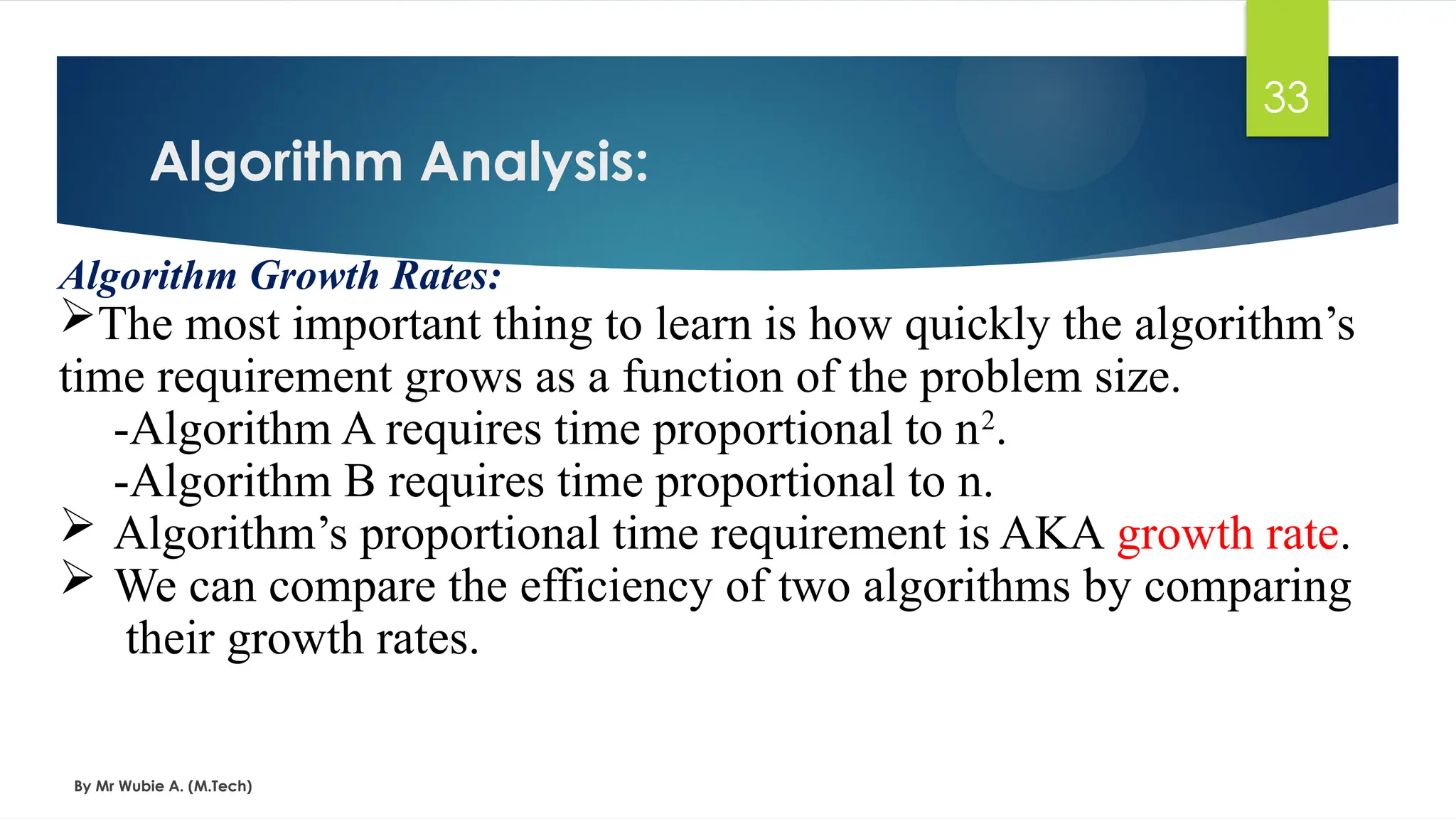
Algorithm Growth Rates:
The most important thing to learn is how quickly the algorithm’s
time requirement grows as a function of the problem size.
-Algorithm A requires time proportional to n2
.
-Algorithm B requires time proportional to n.
 Algorithm’s proportional time requirement is AKA growth rate.
 We can compare the efficiency of two algorithms by comparing
their growth rates.

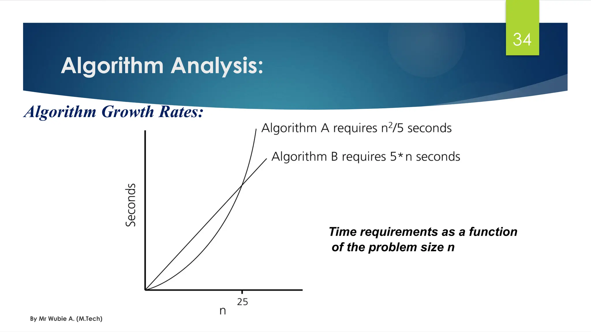
34. Time requirements as a function
of the problem size n
Algorithm Analysis:
By Mr Wubie A. (M.Tech)
34
Algorithm Growth Rates:

35. Asymptotic Analysis:
By Mr Wubie A. (M.Tech)
35
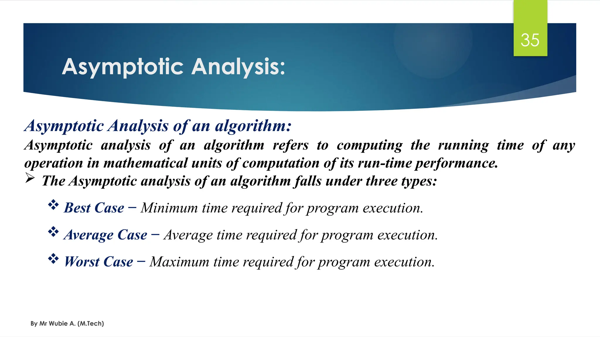
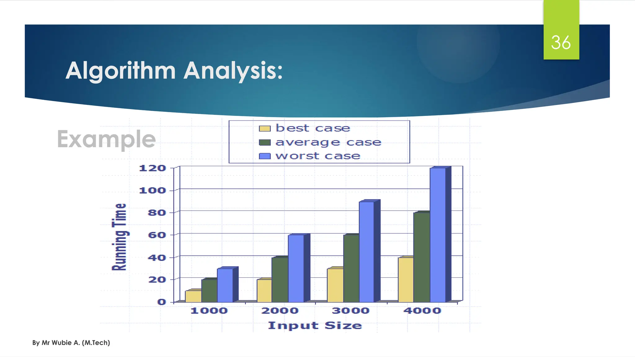
Asymptotic Analysis of an algorithm:
Asymptotic analysis of an algorithm refers to computing the running time of any
operation in mathematical units of computation of its run-time performance.
 The Asymptotic analysis of an algorithm falls under three types:
 Best Case − Minimum time required for program execution.
 Average Case − Average time required for program execution.
 Worst Case − Maximum time required for program execution.

36. Algorithm Analysis:
By Mr Wubie A. (M.Tech)
36
Example

37. Asymptotic Notations:
By Mr Wubie A. (M.Tech)
37
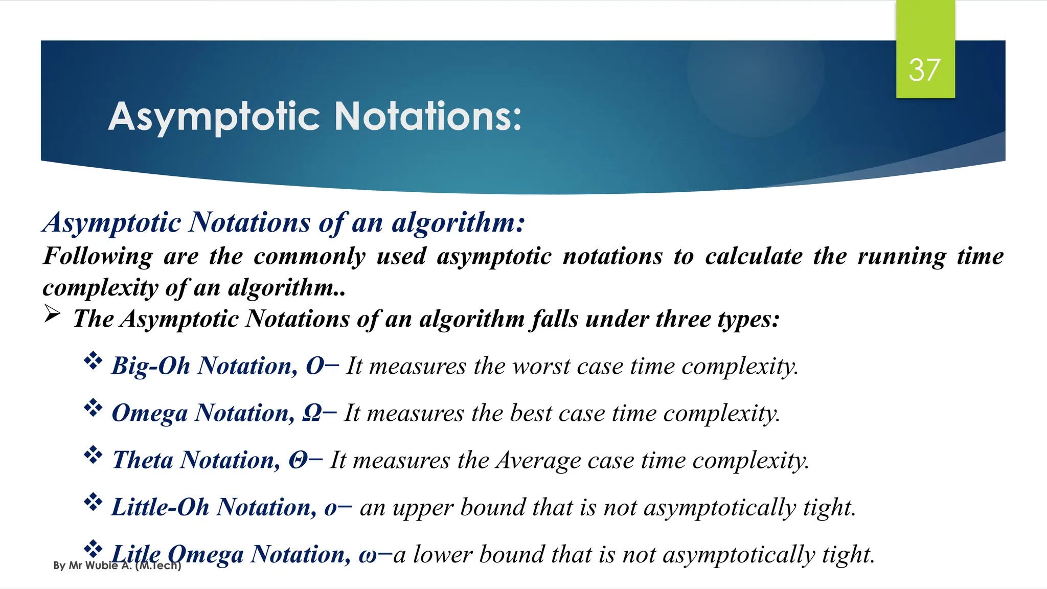
Asymptotic Notations of an algorithm:
Following are the commonly used asymptotic notations to calculate the running time
complexity of an algorithm..
 The Asymptotic Notations of an algorithm falls under three types:
 Big-Oh Notation, Ο− It measures the worst case time complexity.
 Omega Notation, Ω− It measures the best case time complexity.
 Theta Notation, Θ− It measures the Average case time complexity.
 Little-Oh Notation, o− an upper bound that is not asymptotically tight.
 Litle Omega Notation, ω−a lower bound that is not asymptotically tight.

38. Asymptotic Notations:
By Mr Wubie A. (M.Tech)
38
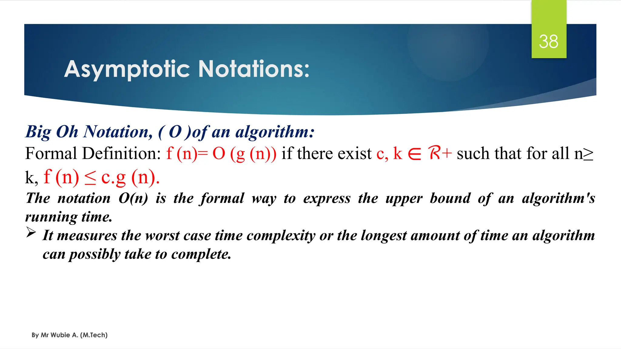
Big Oh Notation, ( Ο )of an algorithm:
Formal Definition: f (n)= O (g (n)) if there exist c, k +
∊ ℛ such that for all n≥
k, f (n) ≤ c.g (n).
The notation Ο(n) is the formal way to express the upper bound of an algorithm's
running time.
 It measures the worst case time complexity or the longest amount of time an algorithm
can possibly take to complete.

39. Asymptotic Notations:
By Mr Wubie A. (M.Tech)
39
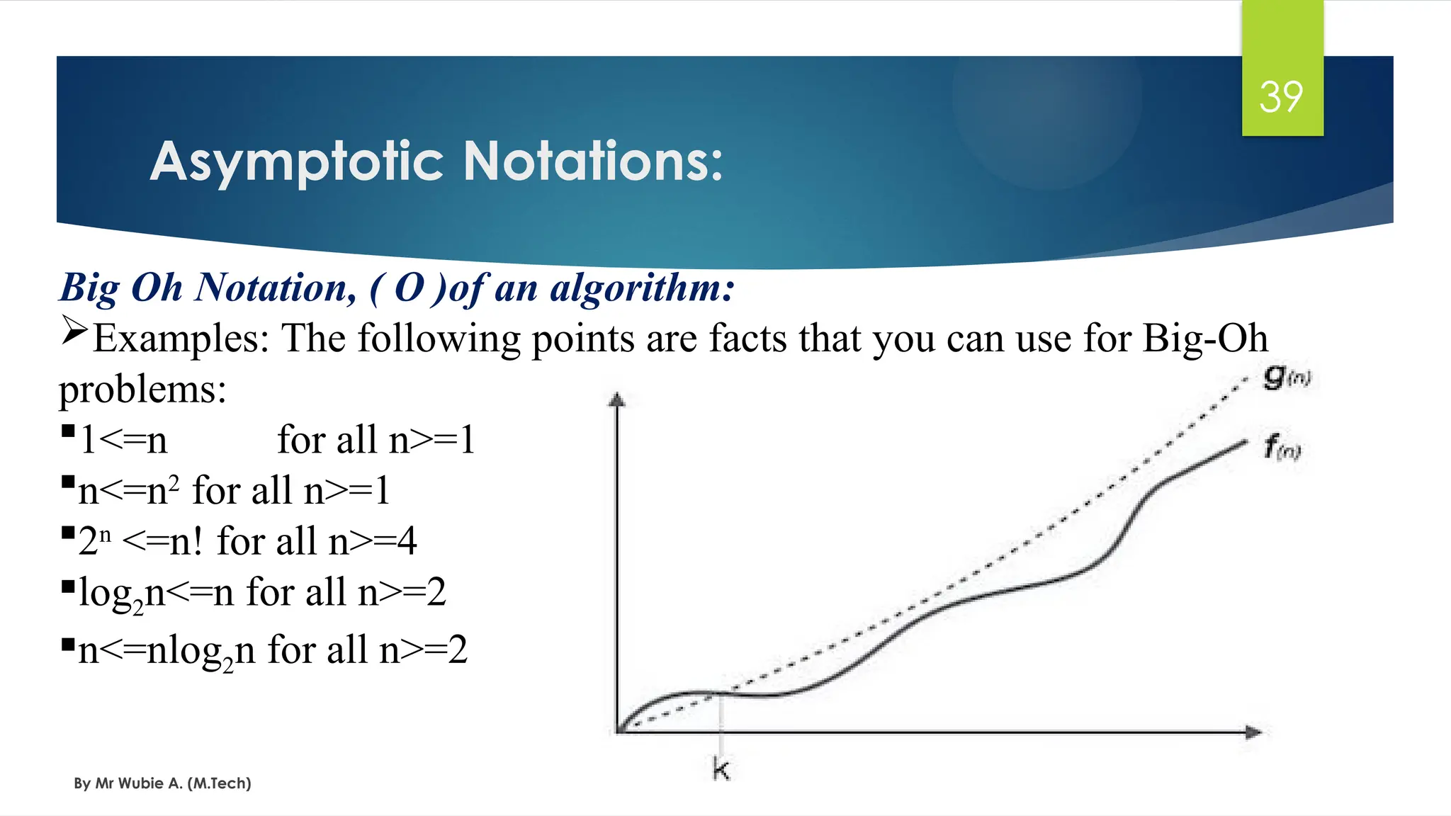
Big Oh Notation, ( Ο )of an algorithm:
Examples: The following points are facts that you can use for Big-Oh
problems:
1<=n for all n>=1
n<=n2
for all n>=1
2n
<=n! for all n>=4
log2n<=n for all n>=2
n<=nlog2n for all n>=2

40. Asymptotic Notations:
By Mr Wubie A. (M.Tech)
40
Big Oh Notation, ( Ο )of an algorithm:
Example 1: f(n)=10n+5 and g(n)=n. Show that f(n) is O(g(n)).
To show that f(n) is O(g(n)) we must show that constants c and k such that
f(n) <=c.g(n) for all n>=k
Or 10n+5<=c.n for all n>=k
Try c=15. Then we need to show that 10n+5<=15n
Solving for n we get: 5<5n or 1<=n.
So f(n) =10n+5 <=15.g(n) for all n>=1.
(c=15,k=1).

41. Asymptotic Notations:
By Mr Wubie A. (M.Tech)
41
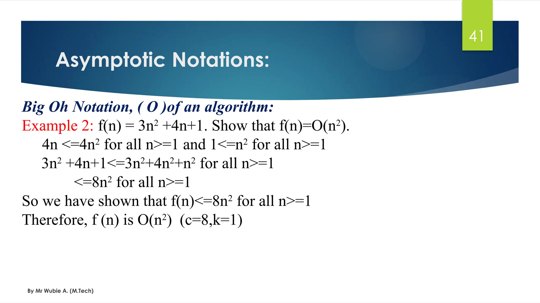
Big Oh Notation, ( Ο )of an algorithm:
Example 2: f(n) = 3n2
+4n+1. Show that f(n)=O(n2
).
4n <=4n2
for all n>=1 and 1<=n2
for all n>=1
3n2
+4n+1<=3n2
+4n2
+n2
for all n>=1
<=8n2
for all n>=1
So we have shown that f(n)<=8n2
for all n>=1
Therefore, f (n) is O(n2
) (c=8,k=1)

42. Omega Notation, Ω of an algorithm:
Formal Definition: A function f(n) is Ω(g(n)) if there exist constants c and k + such
∊ ℛ
that f(n) >=c. g(n) for all n>=k.
 f(n)= Ω(g (n)) means that f(n) is greater than or equal to some constant multiple of g(n)
for all values of n greater than or equal to some k.
Example: If f(n) =n2
, then f(n)= Ω( n)
 In simple terms, f(n)= Ω(g(n)) means that the growth rate of f(n) is greater that or equal
to g(n).
Asymptotic Notations:
By Mr Wubie A. (M.Tech)
42

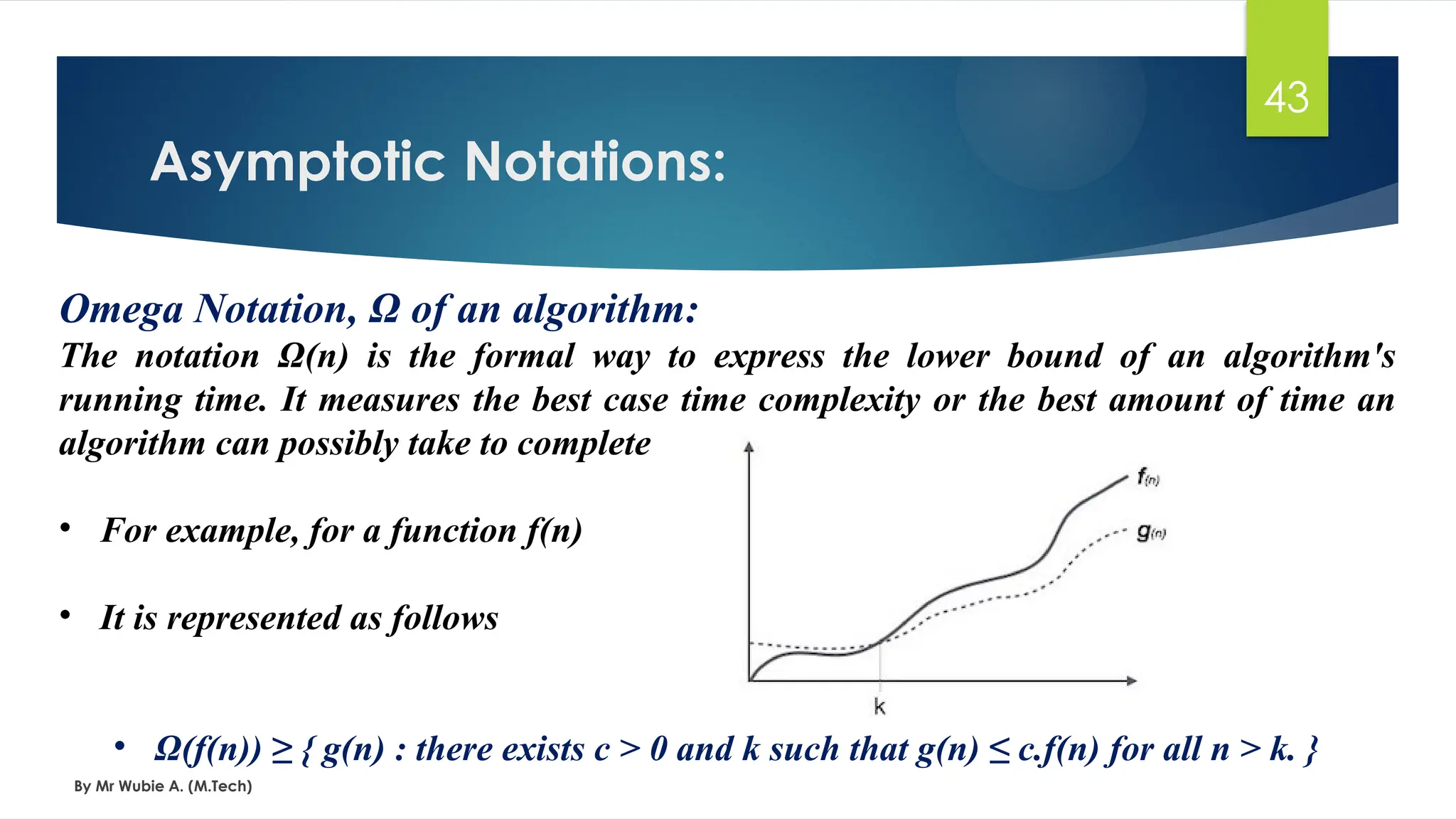
43. Omega Notation, Ω of an algorithm:
The notation Ω(n) is the formal way to express the lower bound of an algorithm's
running time. It measures the best case time complexity or the best amount of time an
algorithm can possibly take to complete
• For example, for a function f(n)
• It is represented as follows
• Ω(f(n)) ≥ { g(n) : there exists c > 0 and k such that g(n) ≤ c.f(n) for all n > k. }
Asymptotic Notations:
By Mr Wubie A. (M.Tech)
43

44. Asymptotic Notations:
By Mr Wubie A. (M.Tech)
44
Theta Notation, Θ of an algorithm:
Formal Definition: A function f (n) is Θ(g(n)) if it is both O(g(n)) and Ω(g(n)). In other
words, there exist constants c1, c2, and k >0 such that c1.g(n) <= f(n) <= c2. g(n) for all
n >= k
If f(n)= Θ(g(n)), then g(n) is an asymptotically tight bound for f(n).
In simple terms, f(n)= Θ(g(n)) means that f(n) and g(n) have the same rate of growth.
Example:
1. If f(n)=2n+1, then f(n) = Θ (n)
2. f(n) =2n2
then f(n)=O(n4
) f(n)=O(n3
) f(n)=O(n2
)
All these are technically correct, but the last expression is the best and tight one. Since 2n2
and n2
have the same growth rate, it can be written as f(n)= Θ(n2
).

45. Asymptotic Notations:
By Mr Wubie A. (M.Tech)
45
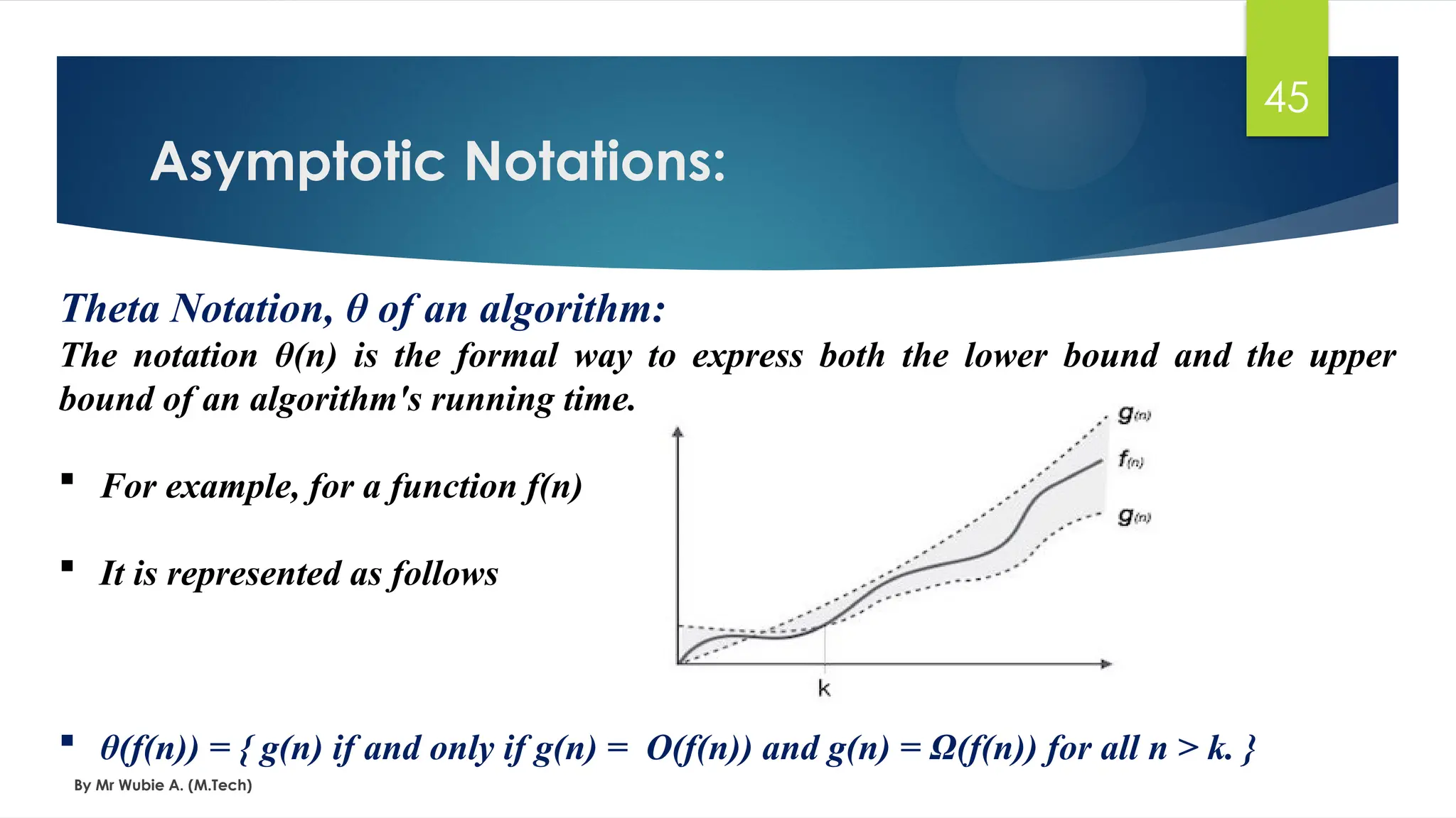
Theta Notation, θ of an algorithm:
The notation θ(n) is the formal way to express both the lower bound and the upper
bound of an algorithm's running time.
 For example, for a function f(n)
 It is represented as follows
 θ(f(n)) = { g(n) if and only if g(n) = Ο(f(n)) and g(n) = Ω(f(n)) for all n > k. }

46. Asymptotic Notations:
By Mr Wubie A. (M.Tech)
46
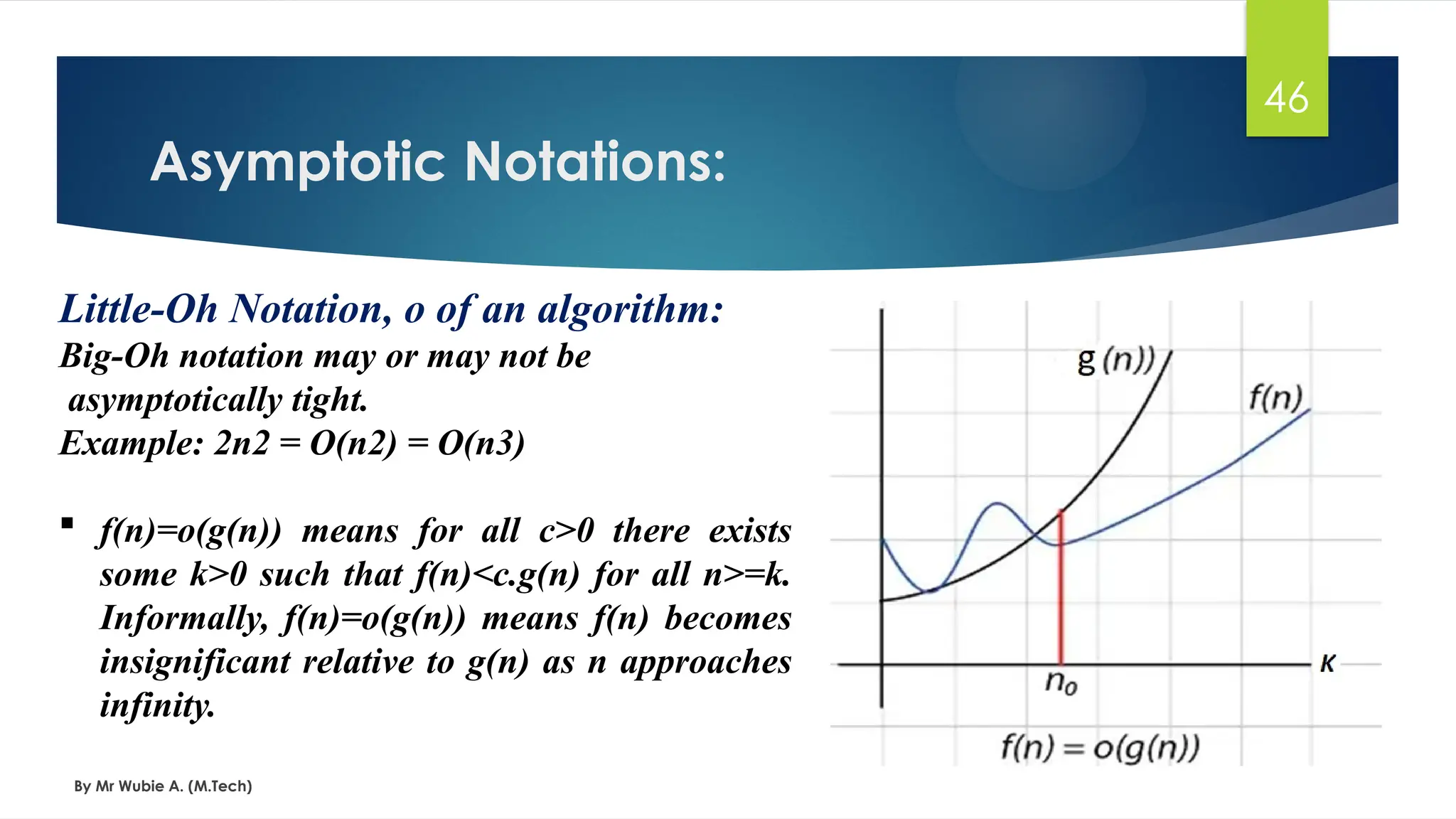
Little-Oh Notation, o of an algorithm:
Big-Oh notation may or may not be
asymptotically tight.
Example: 2n2 = O(n2) = O(n3)
 f(n)=o(g(n)) means for all c>0 there exists
some k>0 such that f(n)<c.g(n) for all n>=k.
Informally, f(n)=o(g(n)) means f(n) becomes
insignificant relative to g(n) as n approaches
infinity.

47. Asymptotic Notations:
By Mr Wubie A. (M.Tech)
47
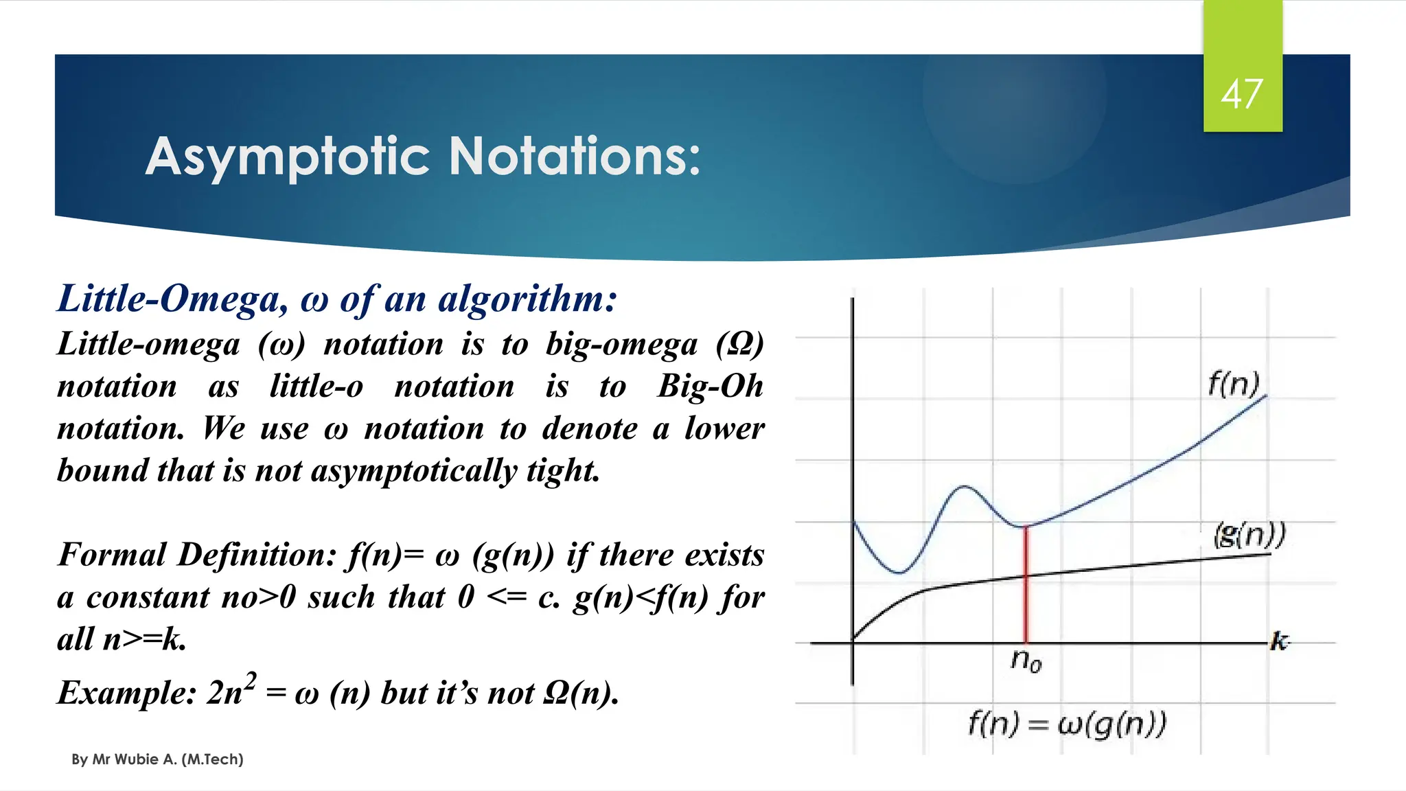
Little-Omega, ω of an algorithm:
Little-omega (ω) notation is to big-omega (Ω)
notation as little-o notation is to Big-Oh
notation. We use ω notation to denote a lower
bound that is not asymptotically tight.
Formal Definition: f(n)= ω (g(n)) if there exists
a constant no>0 such that 0 <= c. g(n)<f(n) for
all n>=k.
Example: 2n2
= ω (n) but it’s not Ω(n).

48. Asymptotic Notations:
By Mr Wubie A. (M.Tech)
48
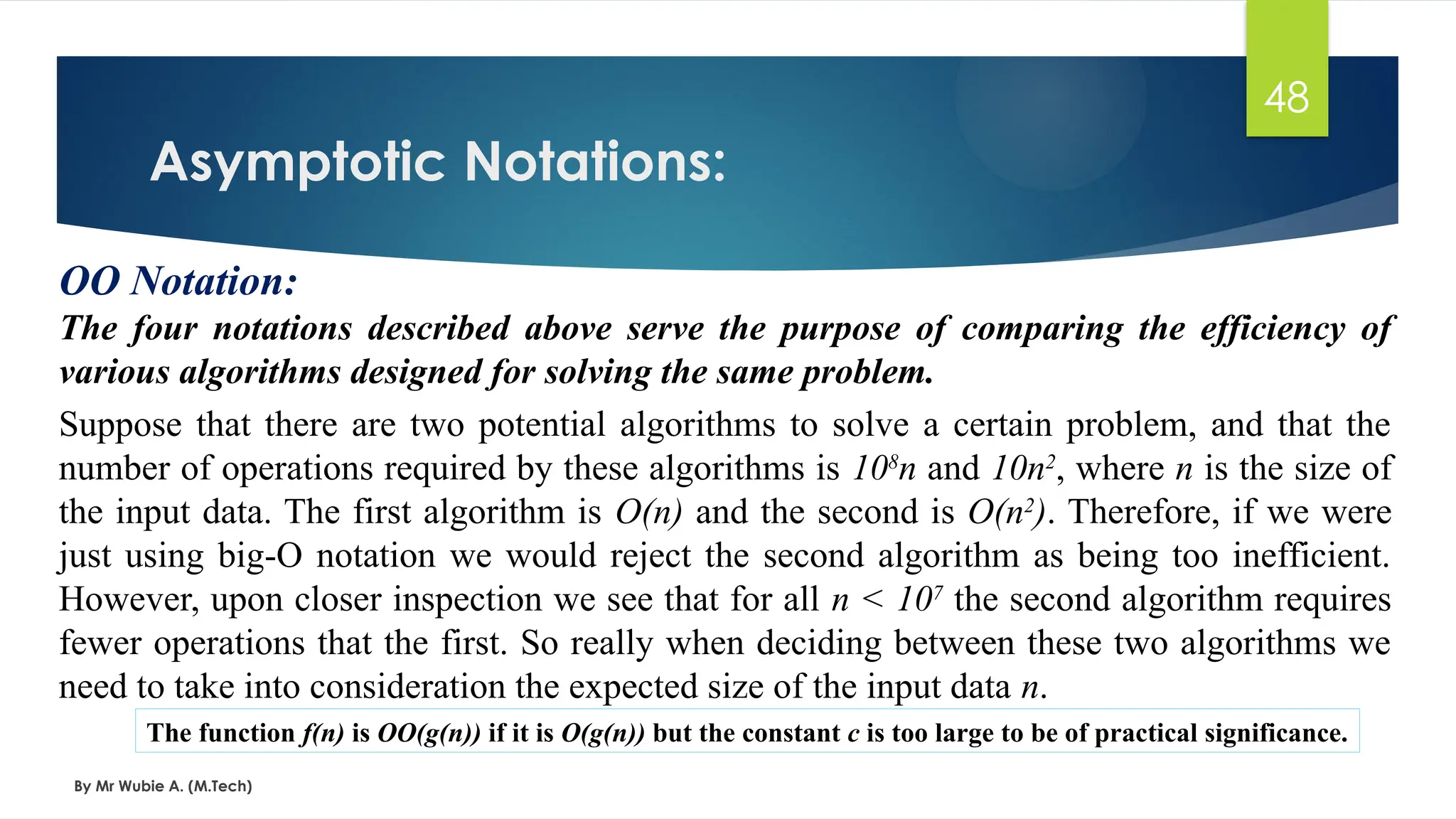
OO Notation:
The four notations described above serve the purpose of comparing the efficiency of
various algorithms designed for solving the same problem.
Suppose that there are two potential algorithms to solve a certain problem, and that the
number of operations required by these algorithms is 108
n and 10n2
, where n is the size of
the input data. The first algorithm is O(n) and the second is O(n2
). Therefore, if we were
just using big-O notation we would reject the second algorithm as being too inefficient.
However, upon closer inspection we see that for all n < 107
the second algorithm requires
fewer operations that the first. So really when deciding between these two algorithms we
need to take into consideration the expected size of the input data n.
The function f(n) is OO(g(n)) if it is O(g(n)) but the constant c is too large to be of practical significance.

49. Complexity Classes:
By Mr Wubie A. (M.Tech)
49
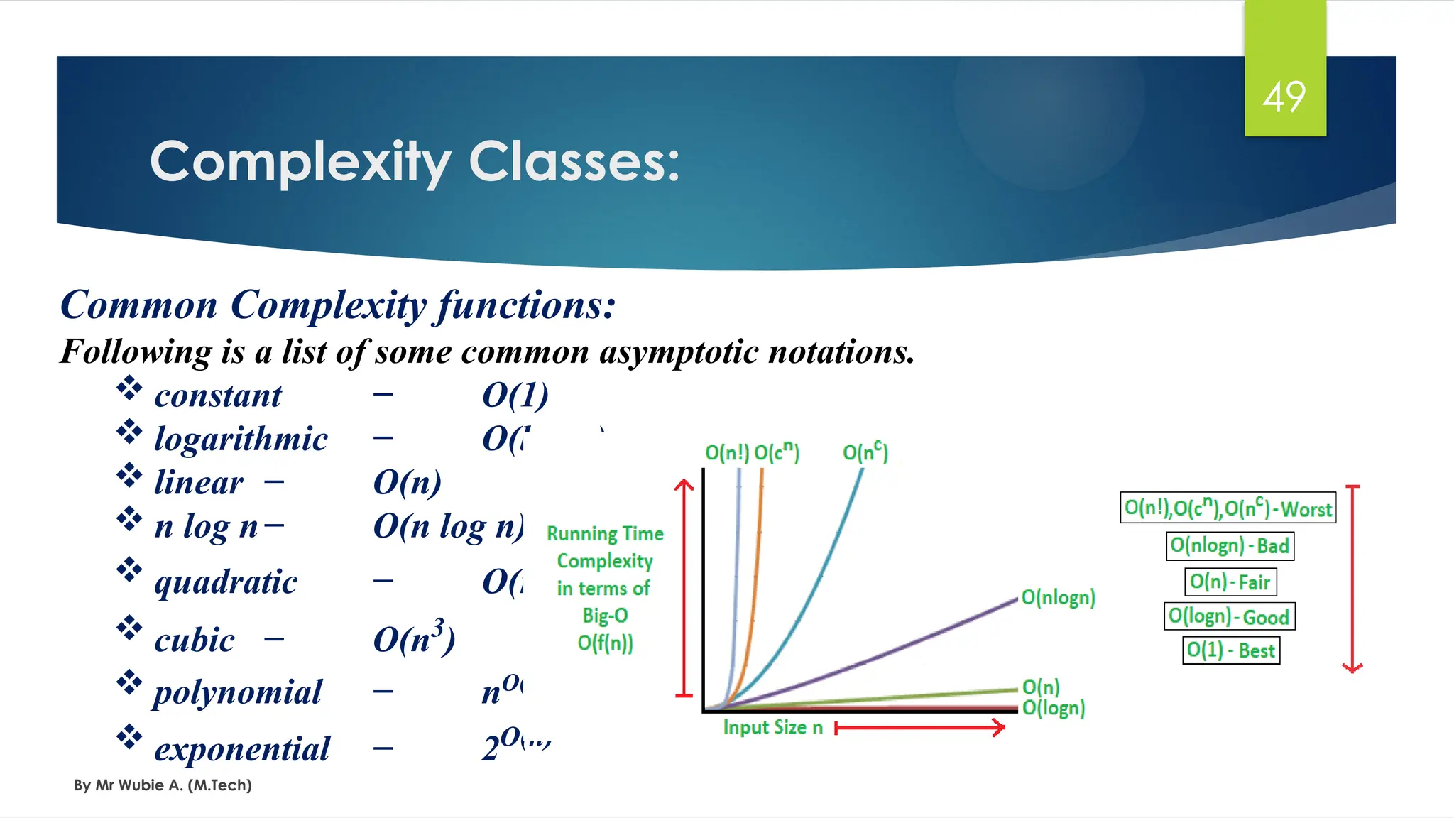
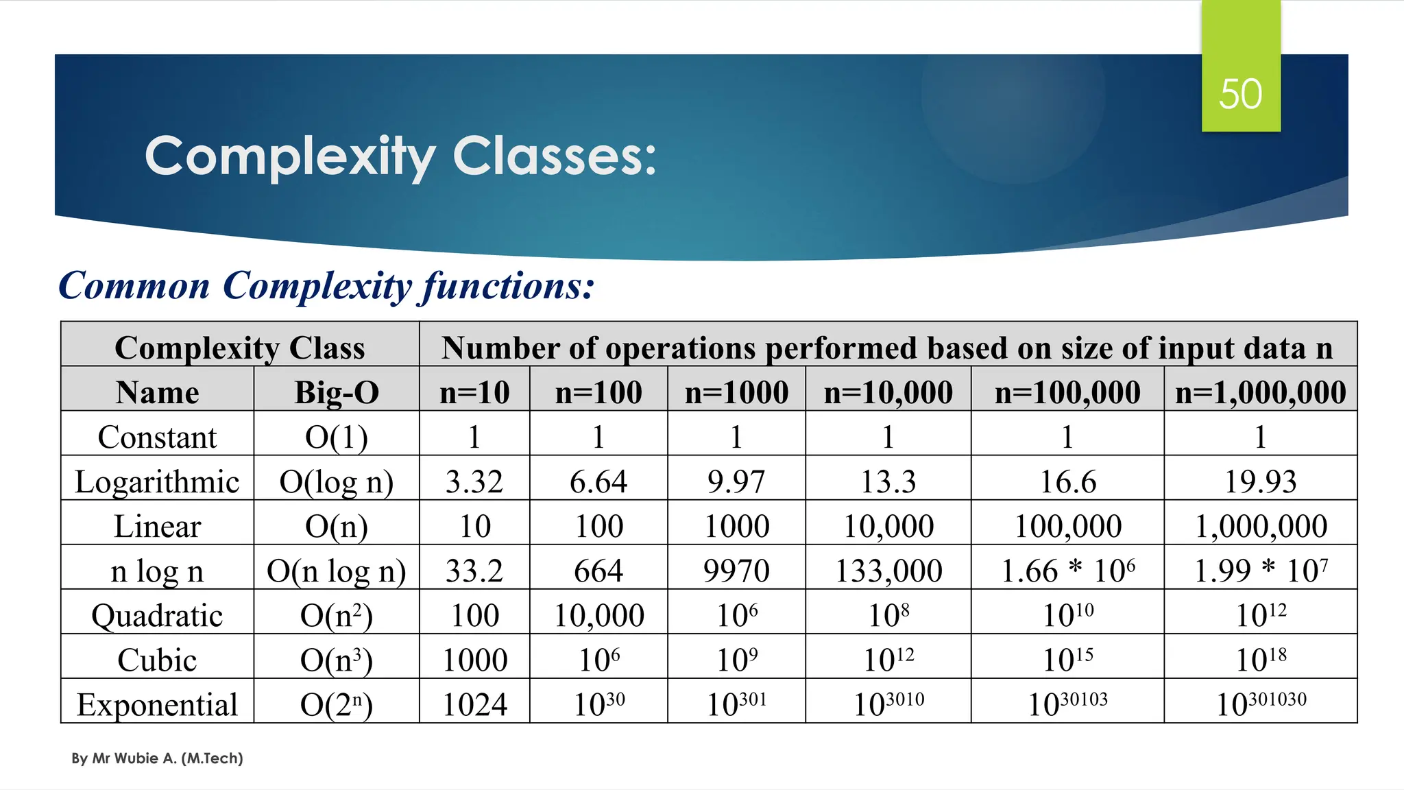
Common Complexity functions:
Following is a list of some common asymptotic notations.
 constant − Ο(1)
 logarithmic − Ο(log n)
 linear − Ο(n)
 n log n− Ο(n log n)
 quadratic − Ο(n2
)
 cubic − Ο(n3
)
 polynomial − nΟ(1)
 exponential − 2Ο(n)

50. Complexity Classes:
By Mr Wubie A. (M.Tech)
50
Common Complexity functions:
Complexity Class Number of operations performed based on size of input data n
Name Big-O n=10 n=100 n=1000 n=10,000 n=100,000 n=1,000,000
Constant O(1) 1 1 1 1 1 1
Logarithmic O(log n) 3.32 6.64 9.97 13.3 16.6 19.93
Linear O(n) 10 100 1000 10,000 100,000 1,000,000
n log n O(n log n) 33.2 664 9970 133,000 1.66 * 106
1.99 * 107
Quadratic O(n2
) 100 10,000 106
108
1010
1012
Cubic O(n3
) 1000 106
109
1012
1015
1018
Exponential O(2n
) 1024 1030
10301
103010
1030103
10301030

51. Amortized Complexity:
By Mr Wubie A. (M.Tech)
51
Amortization:
Amortized complexity refers to the average cost per operation over a sequence of
operations in an algorithm or data structure. Instead of focusing on the worst-case or
best-case scenario for individual operations, amortized analysis provides a more realistic
measure of efficiency by spreading the occasional expensive operations across many
cheaper ones.
 For example: In a dynamic array, most insertions cost O(1), but occasionally, when
the array is full, resizing it (doubling its size) costs O(n). Amortized complexity
considers the overall cost, showing that the average cost remains O(1) per operation
over time.
 This approach is especially useful when analyzing algorithms that involve sequences of
related operations, as it gives a better sense of their long-term efficiency.

52. Amortized Complexity:
By Mr Wubie A. (M.Tech)
52
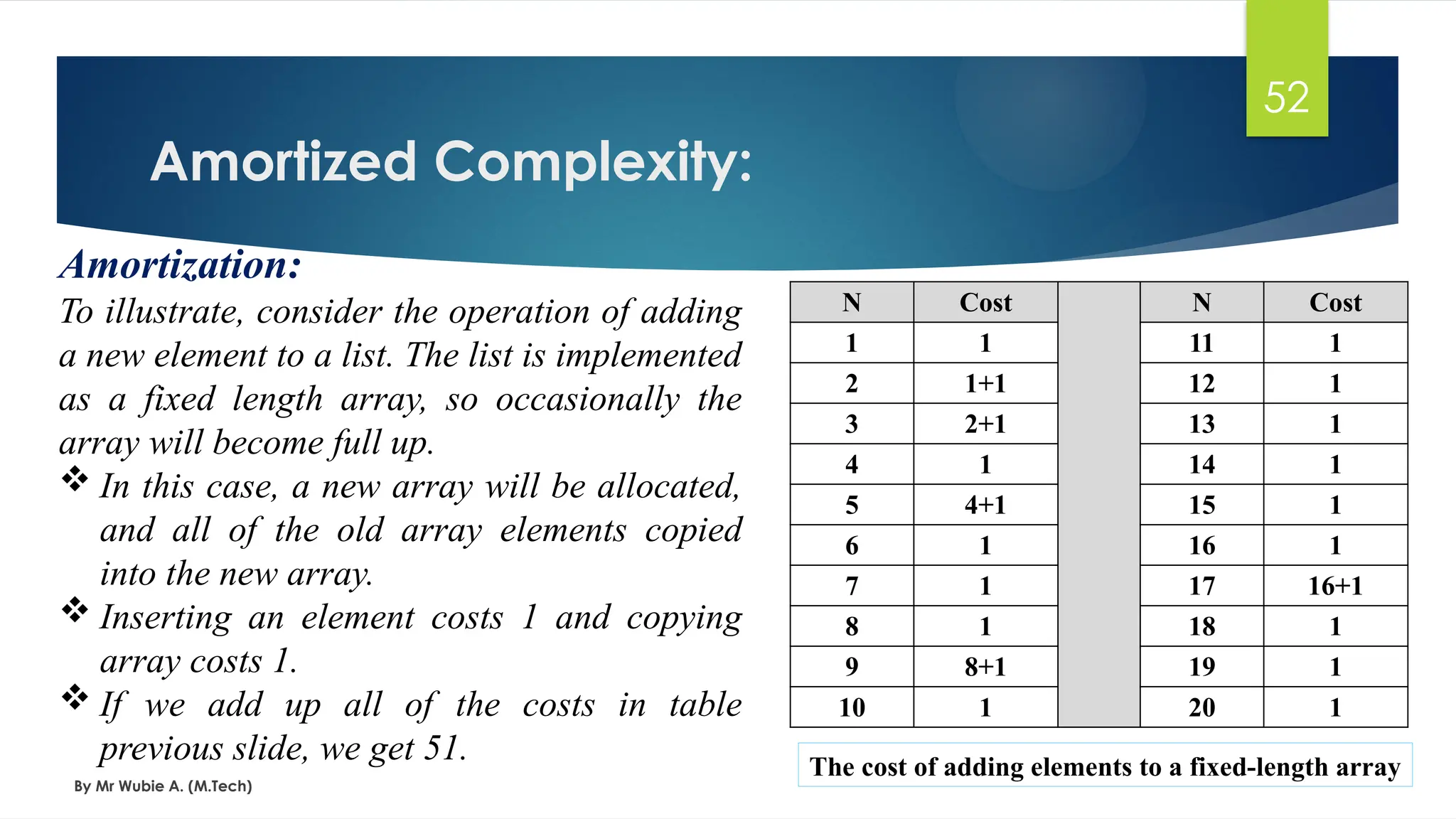
Amortization:
To illustrate, consider the operation of adding
a new element to a list. The list is implemented
as a fixed length array, so occasionally the
array will become full up.
 In this case, a new array will be allocated,
and all of the old array elements copied
into the new array.
 Inserting an element costs 1 and copying
array costs 1.
 If we add up all of the costs in table
previous slide, we get 51.
N Cost N Cost
1 1 11 1
2 1+1 12 1
3 2+1 13 1
4 1 14 1
5 4+1 15 1
6 1 16 1
7 1 17 16+1
8 1 18 1
9 8+1 19 1
10 1 20 1
The cost of adding elements to a fixed-length array

53. Amortized Complexity:
By Mr Wubie A. (M.Tech)
53
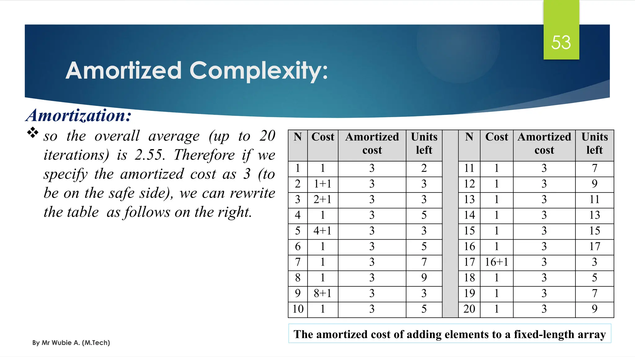
Amortization:
 so the overall average (up to 20
iterations) is 2.55. Therefore if we
specify the amortized cost as 3 (to
be on the safe side), we can rewrite
the table as follows on the right.
The amortized cost of adding elements to a fixed-length array
N Cost Amortized
cost
Units
left
N Cost Amortized
cost
Units
left
1 1 3 2 11 1 3 7
2 1+1 3 3 12 1 3 9
3 2+1 3 3 13 1 3 11
4 1 3 5 14 1 3 13
5 4+1 3 3 15 1 3 15
6 1 3 5 16 1 3 17
7 1 3 7 17 16+1 3 3
8 1 3 9 18 1 3 5
9 8+1 3 3 19 1 3 7
10 1 3 5 20 1 3 9

54. Amortized Complexity:
By Mr Wubie A. (M.Tech)
54
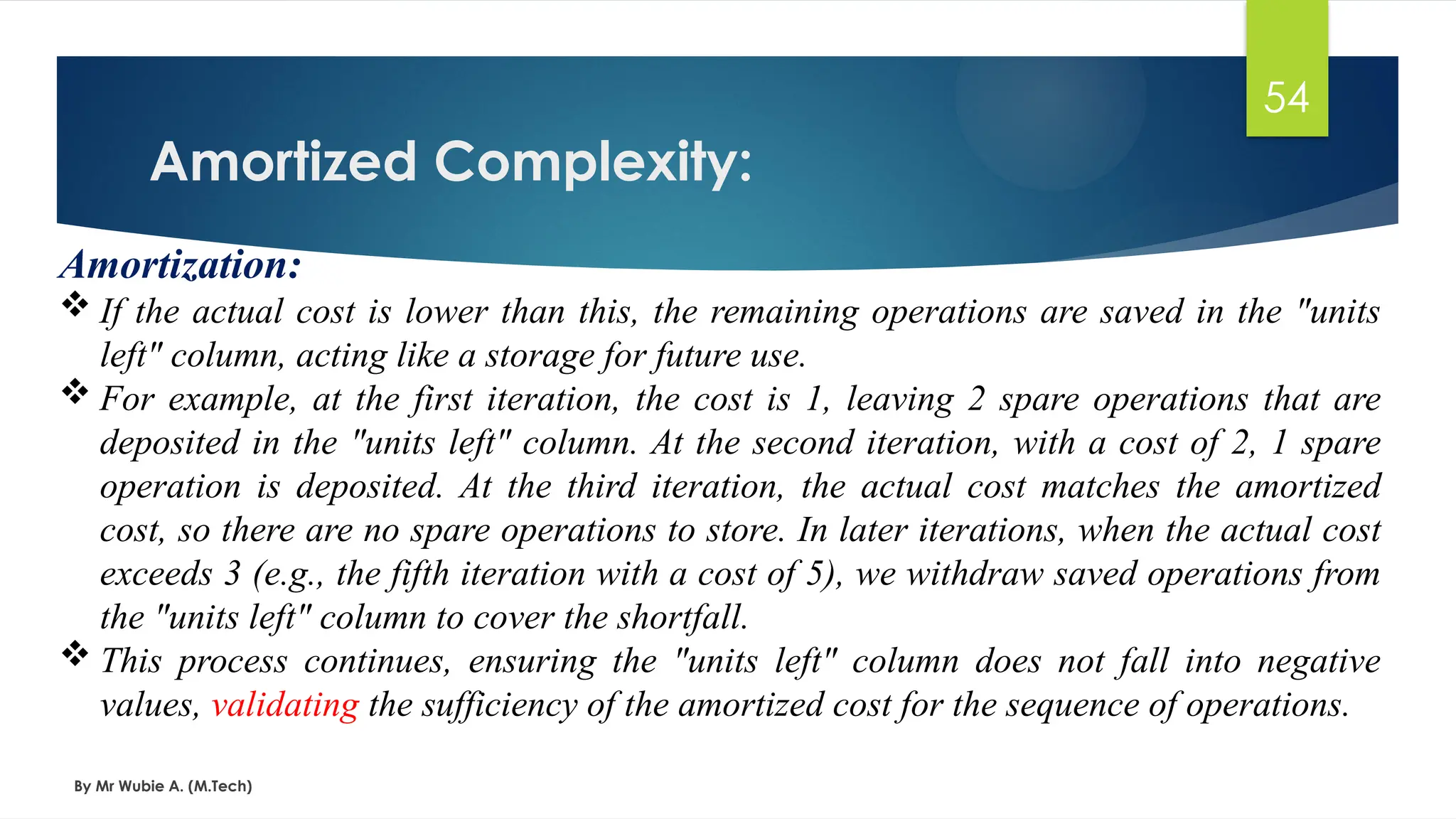
Amortization:
 If the actual cost is lower than this, the remaining operations are saved in the "units
left" column, acting like a storage for future use.
 For example, at the first iteration, the cost is 1, leaving 2 spare operations that are
deposited in the "units left" column. At the second iteration, with a cost of 2, 1 spare
operation is deposited. At the third iteration, the actual cost matches the amortized
cost, so there are no spare operations to store. In later iterations, when the actual cost
exceeds 3 (e.g., the fifth iteration with a cost of 5), we withdraw saved operations from
the "units left" column to cover the shortfall.
 This process continues, ensuring the "units left" column does not fall into negative
values, validating the sufficiency of the amortized cost for the sequence of operations.

55. Data structures
Prof. K. Adisesha (Ph. D)
55
Thank you:
All the best!