


![CSP Potential
200000
175000
150000
Area [km²]
125000
Area with certain
100000
75000
level of solar radiation
50000
25000
0
1800 1900 2000 2100 2200 2300 2400 2500 2600 2700 2800 >
2800
Electricity Potential [TWh/y]
DNI [kWh/m²a] 25000
20000
15000
10000
Technical potential
5000
calc. with power plant model
0
00
00
00
00
00
00
00
00
00
00
00
00
28
18
19
20
21
22
23
24
25
26
27
28
>
Folie 55](https://image.slidesharecdn.com/introductiontosolarresouceassessments-130102070343-phpapp01/75/Introduction-to-solar-resouce-assessments-55-2048.jpg)
![Coastal Potential in Egypt
Coastal Potential - Egypt (20 m a. s. l.)
180
Electricity Potential [TWh/y]
160
140
120
100
2008 power demand
80
60
40
20
0
00
00
00
00
00
00
00
00
00
00
> 0
00
0
18
19
20
21
22
23
24
25
26
27
28
28
DNI [kWh/m²a]
Folie 57](https://image.slidesharecdn.com/introductiontosolarresouceassessments-130102070343-phpapp01/75/Introduction-to-solar-resouce-assessments-57-2048.jpg)
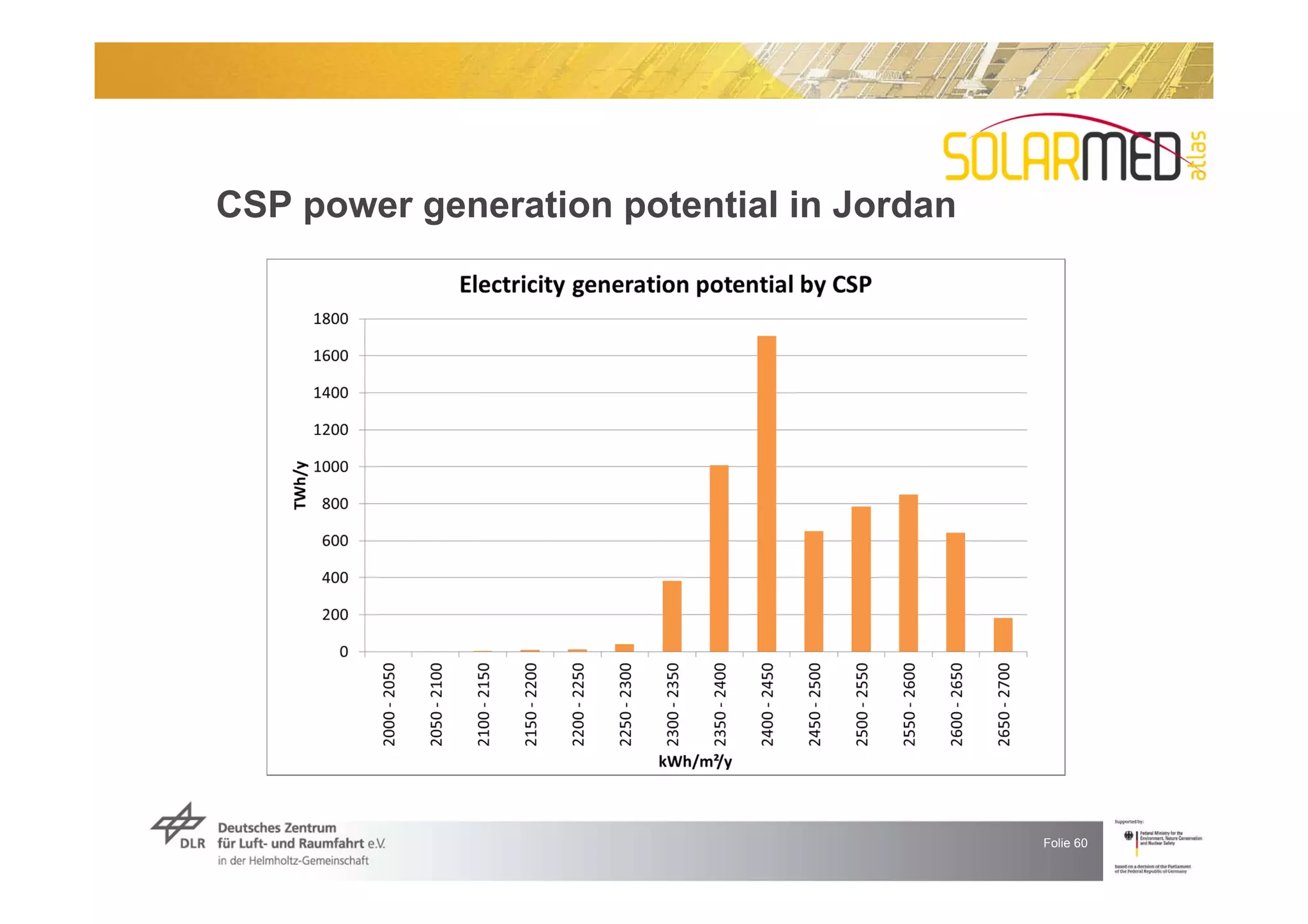
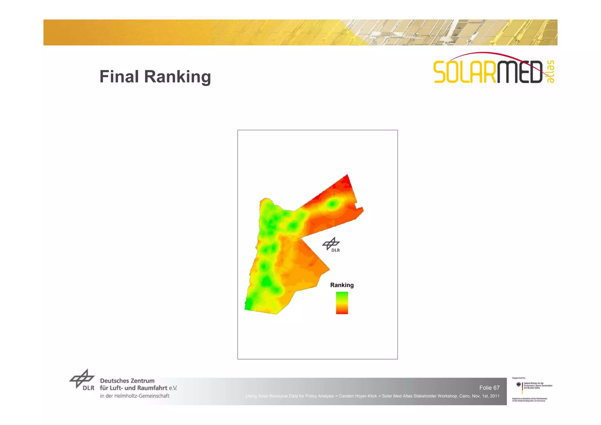
![Potential of Concentrating Solar Power
in Jordan DNI Classes
• Demand 2050: 53 TWh/y [kWh/m²/y]
• Potential CSP: 5884 TWh/y < 1900
1,900
2,000
2,100
2,200
2,300
2,400
2,500
2,600
2,700
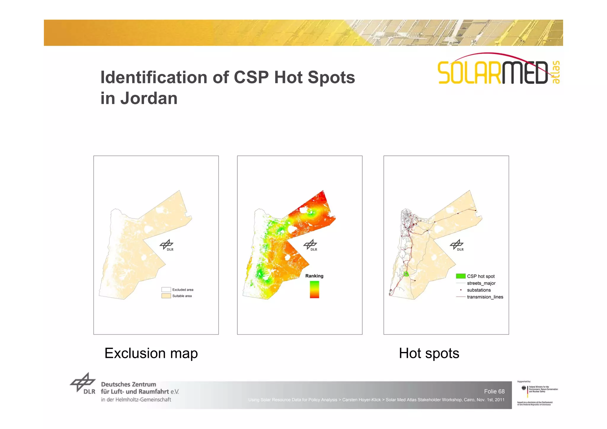
Exclusion Criteria
Urban areas
Population density
Hydrography
Land cover
Protected areas
Topography
Folie 59](https://image.slidesharecdn.com/introductiontosolarresouceassessments-130102070343-phpapp01/75/Introduction-to-solar-resouce-assessments-59-2048.jpg)
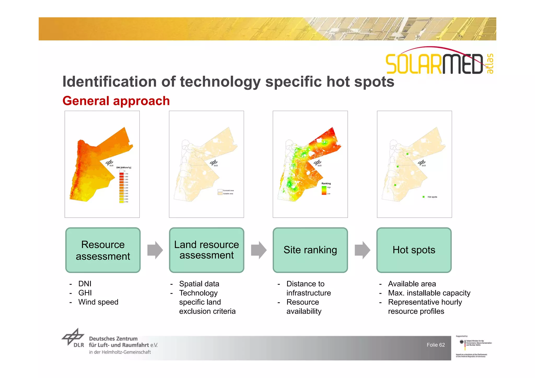

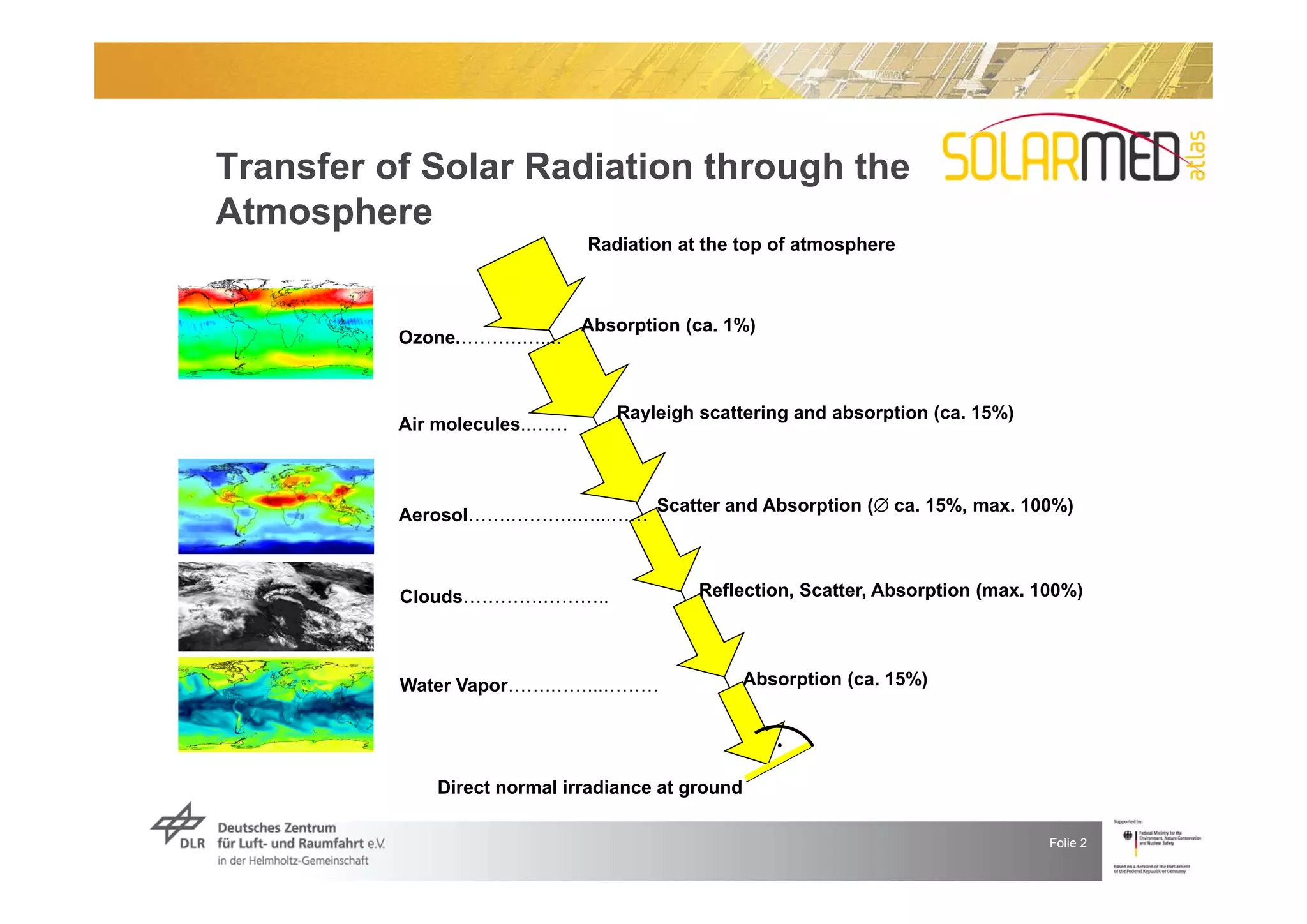
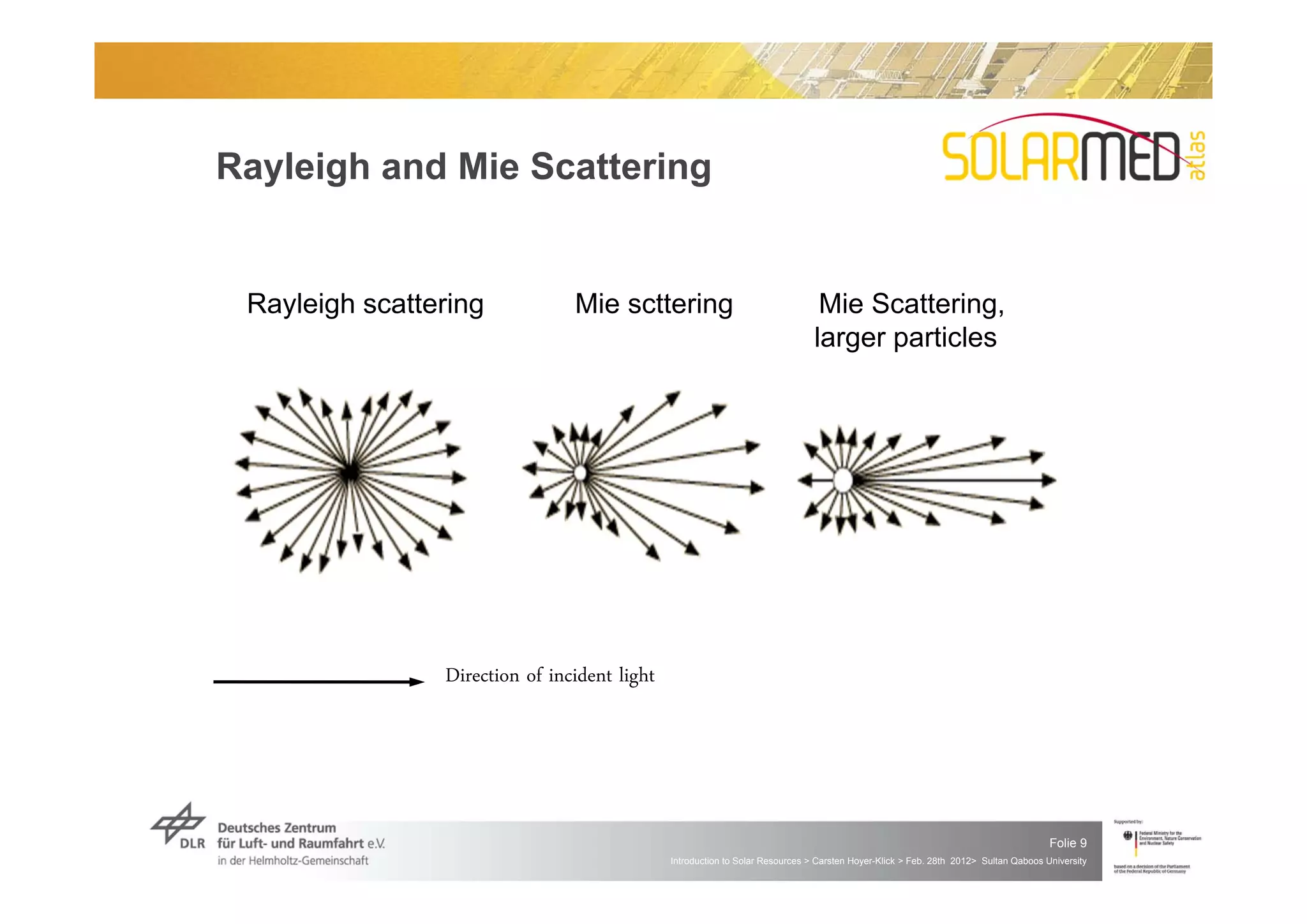
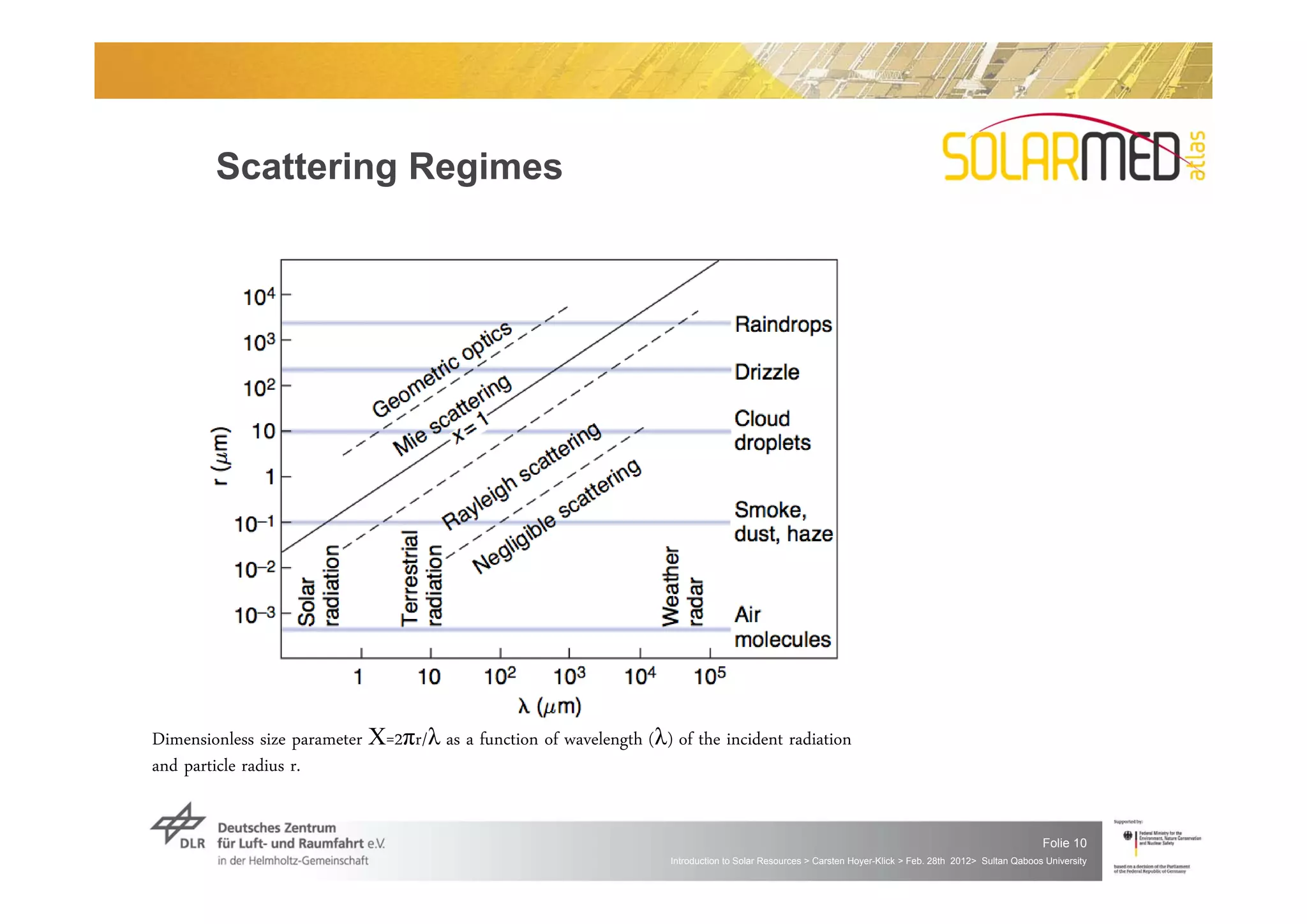
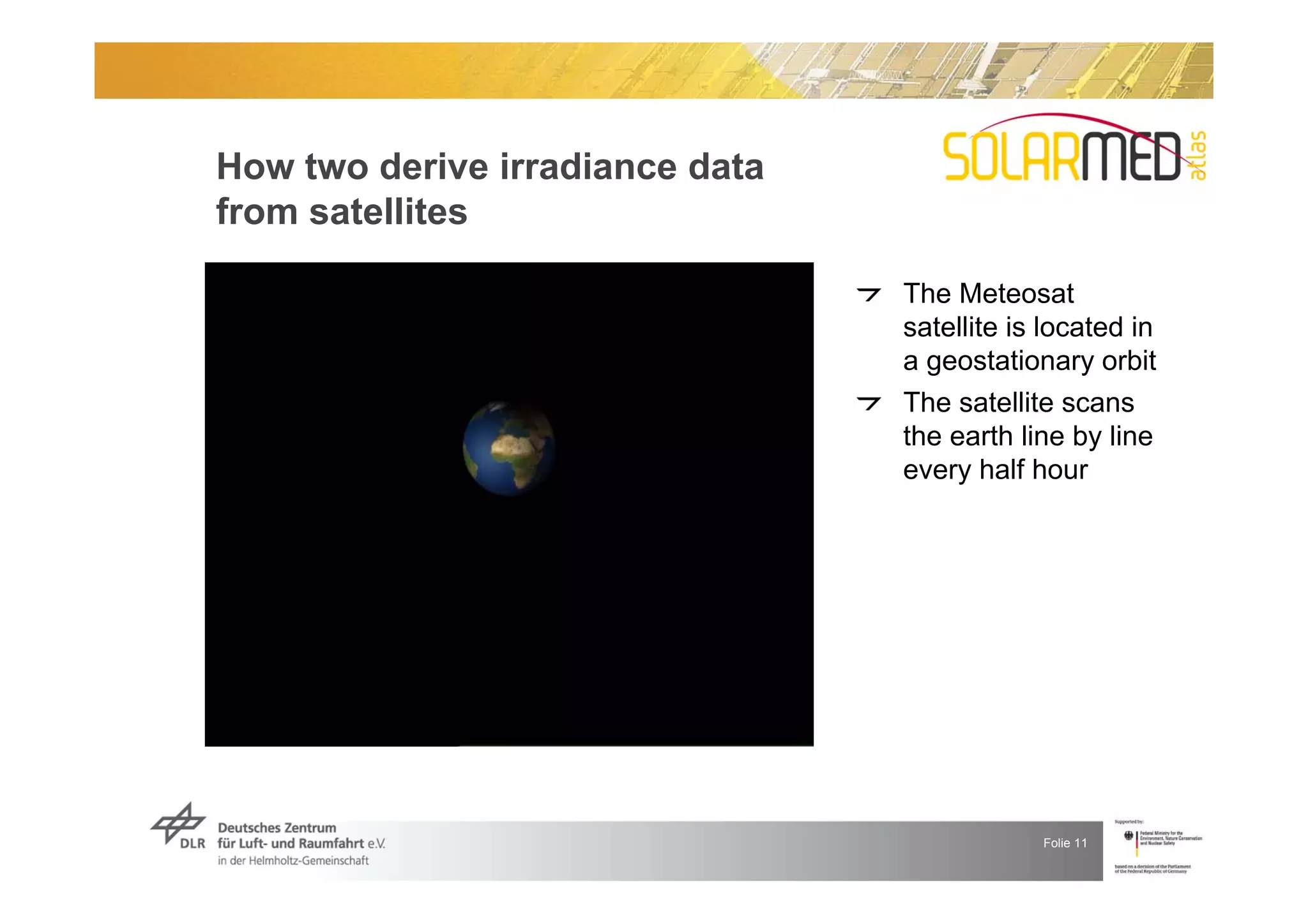
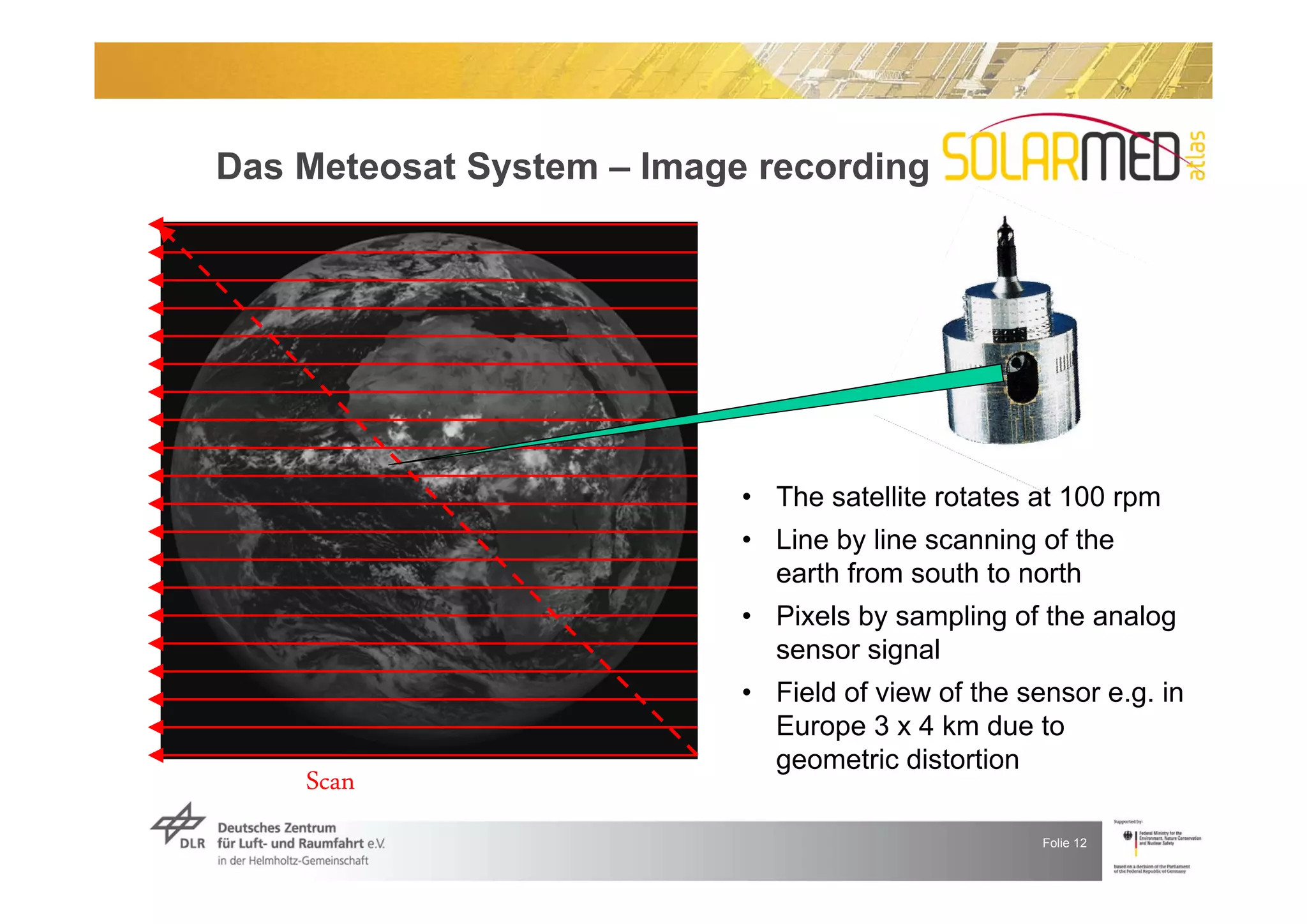
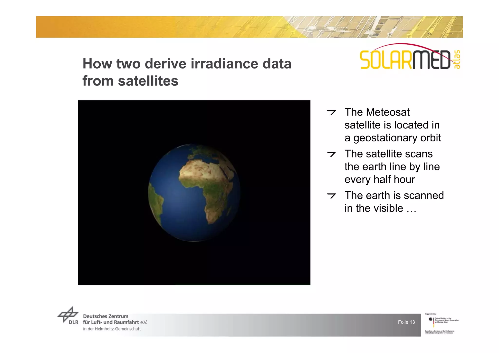
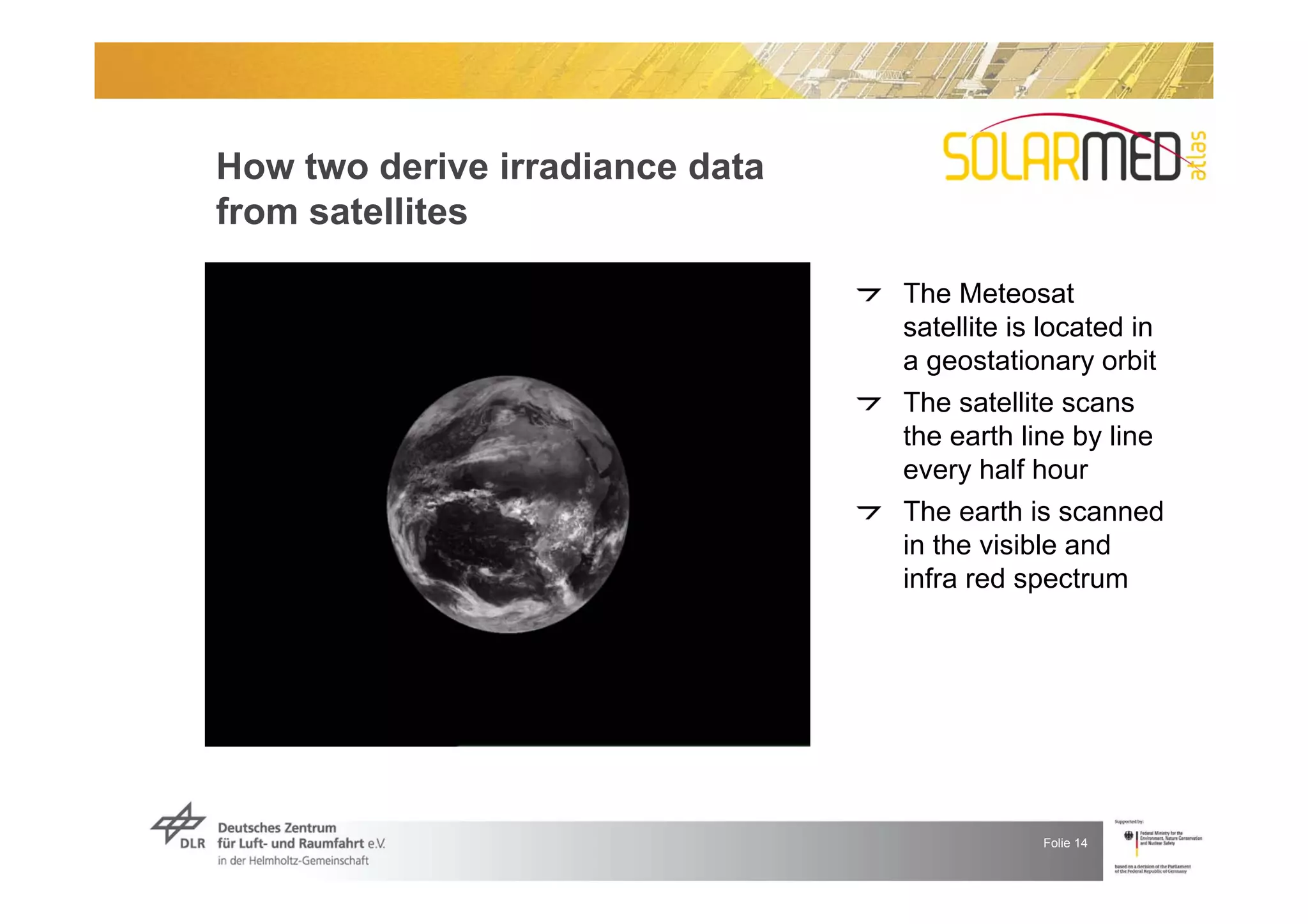
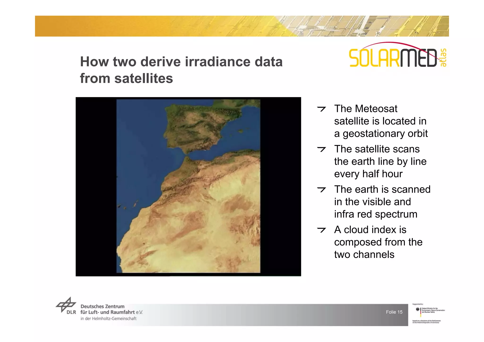
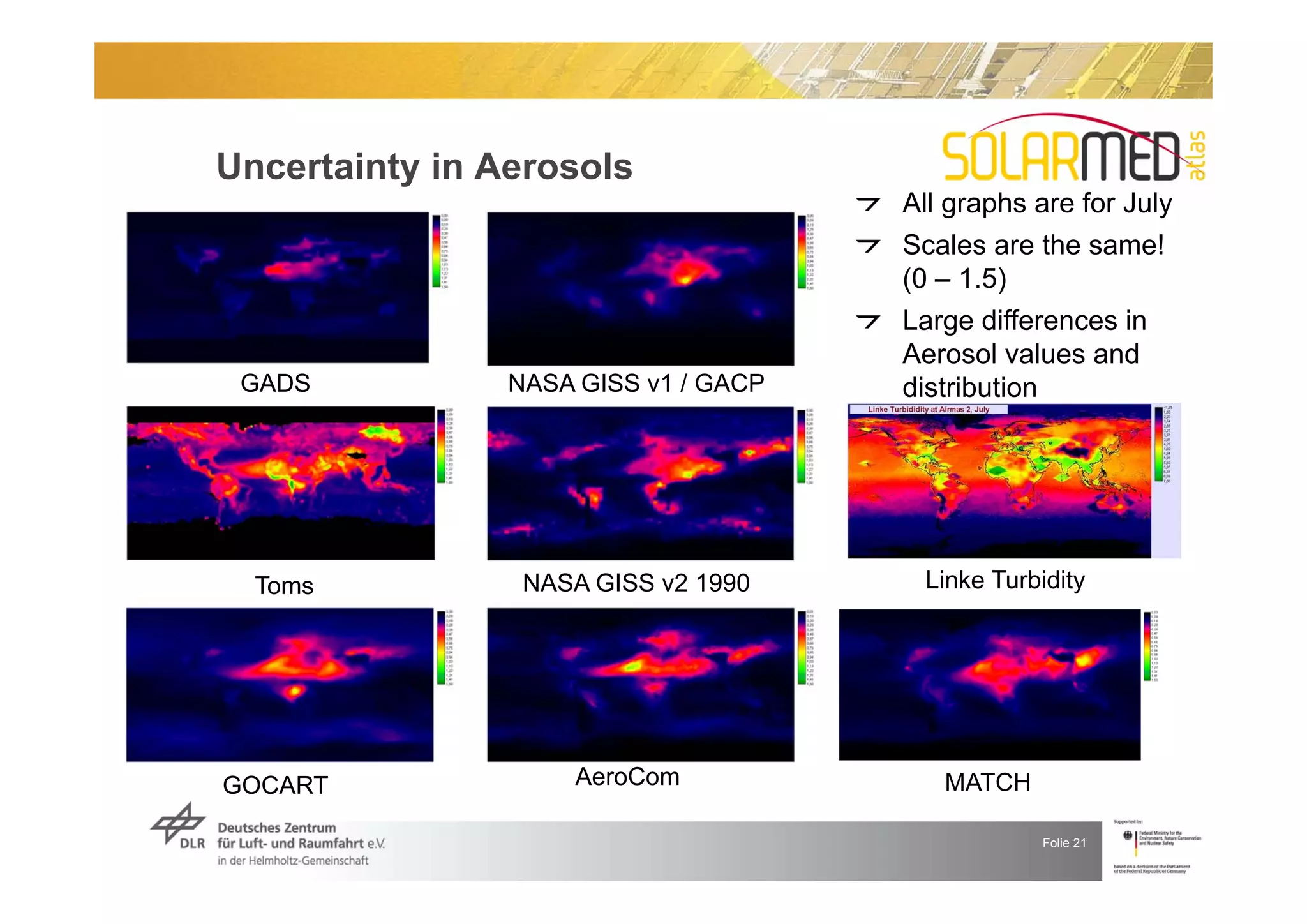
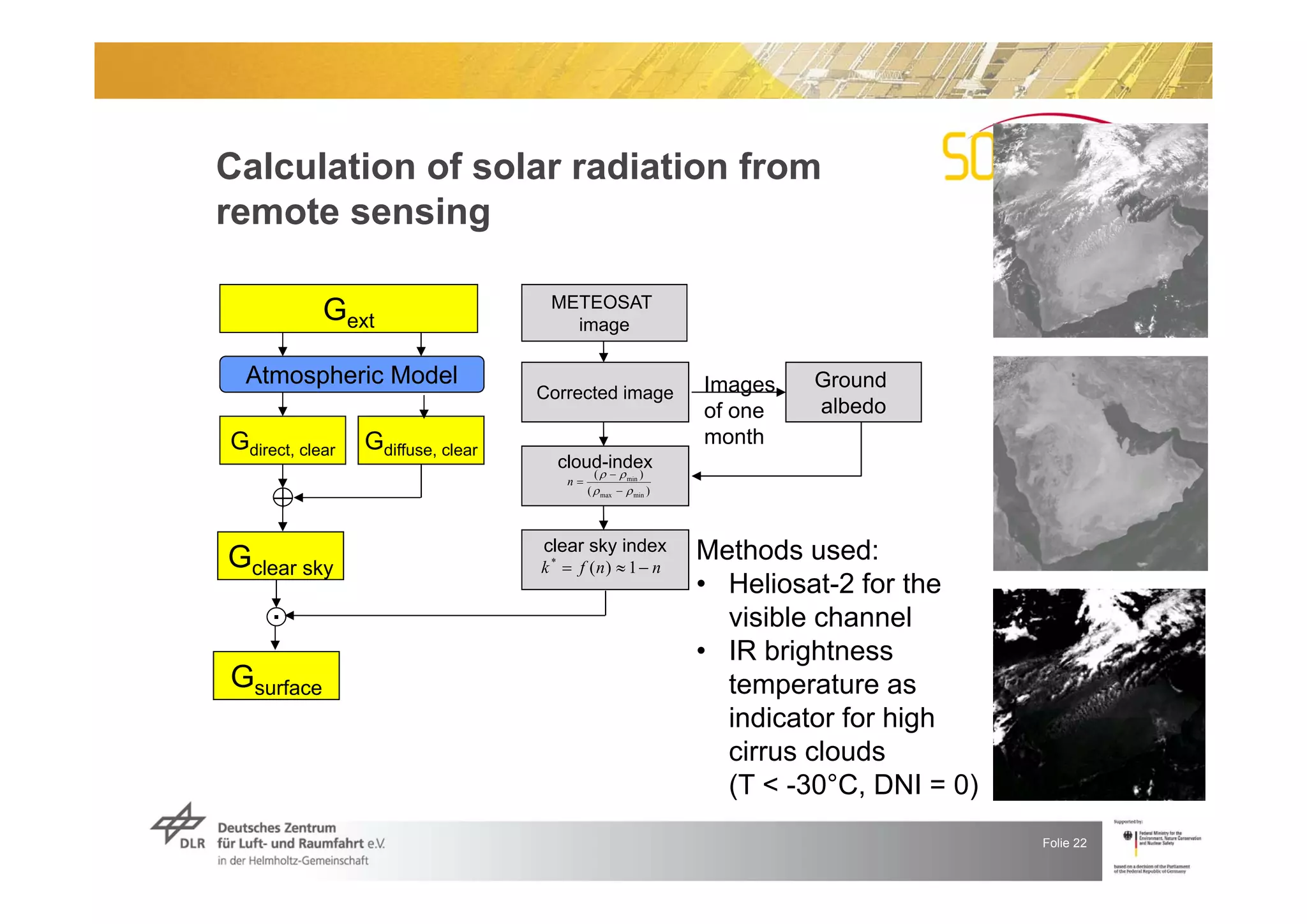
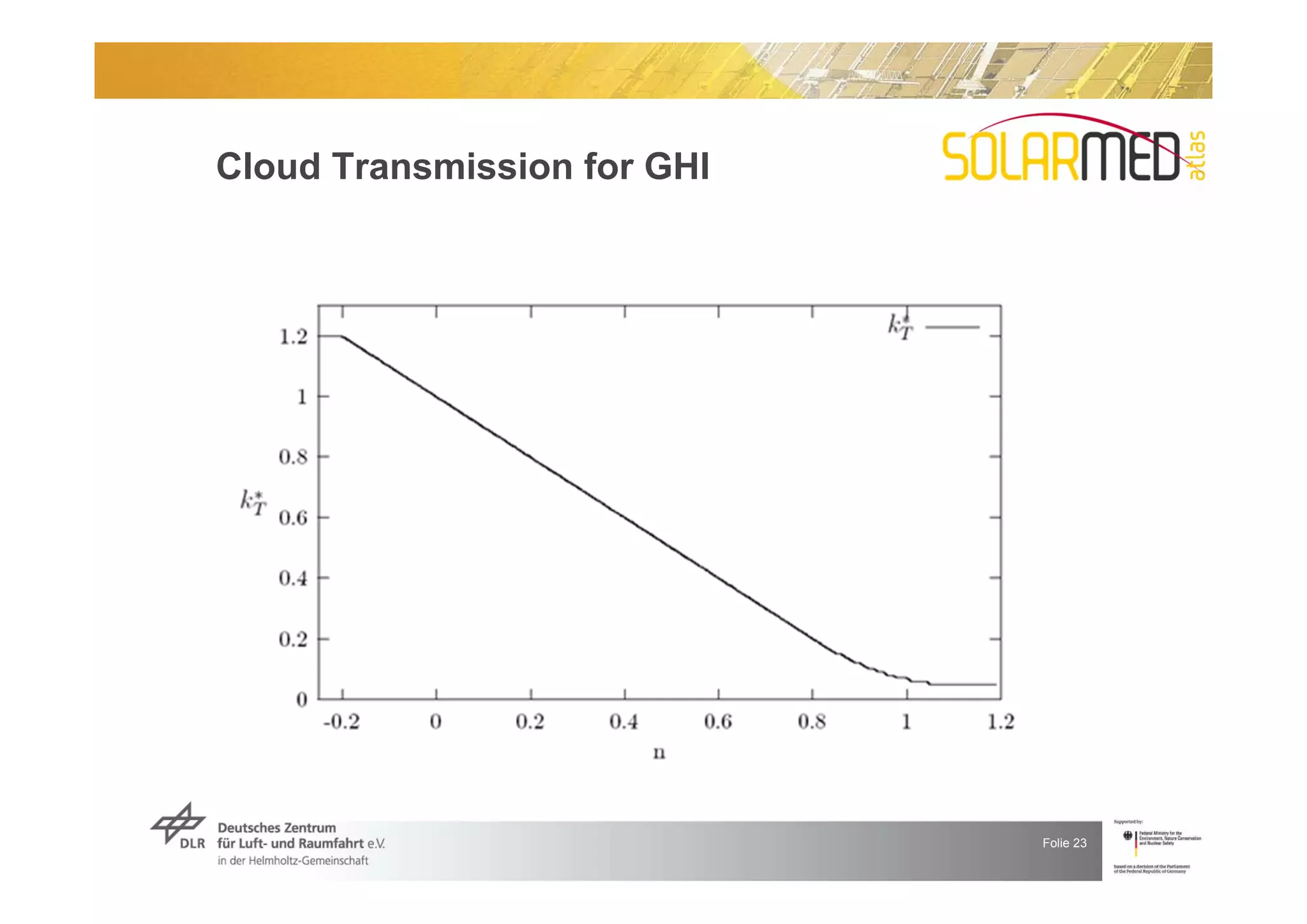
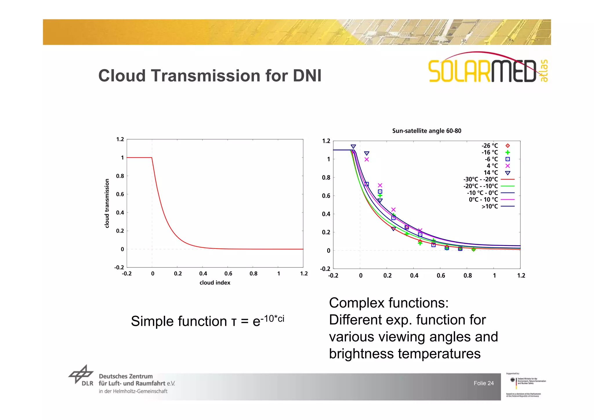
The document introduces solar resource assessments through satellite data. It discusses how satellites like Meteosat scan the Earth's surface to measure solar irradiance, and how these measurements are used along with atmospheric models and ground data to estimate solar resources. Key factors that influence solar radiation reaching the surface like aerosols, clouds, and water vapor are also summarized. The document then shows how satellite data can be used to analyze solar potentials and identify prime areas for solar technologies.


