Matematika Keuangan

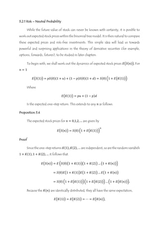
1. 3.2.1 Risk – Neutral Probability
While the future value of stock can never be known with certainty, it is posible to
work out expected stock prices within the binomial tree model. It is then natural to compare
these expected prices and risk-free investments. This simple idea will lead us towards
powerful and surprising applications in the theory of derivative securities (for example,
options, forwards, futures), to be studied in later chapters.
To begin with, we shall work out the dynamics of expected stock prices 𝐸(𝑆(𝑛)). For
𝑛 = 1
𝐸(𝑆(1)) = 𝑝𝑆(0)(1 + 𝑢) + (1 − 𝑝)𝑆(0)(1 + 𝑑) = 𝑆(0) (1 + 𝐸(𝐾(1)))
Where
𝐸(𝐾(1)) = 𝑝𝑢 + (1 − 𝑝)𝑑
Is the expected one-step return. This extends to any 𝑛 as follows.
Proposition 3.4
The expected stock prices for 𝑛 = 0,1,2, … are given by
𝐸(𝑆(𝑛)) = 𝑆(0) (1 + 𝐸(𝐾(1)))
𝑛
Proof
Since the one-step returns 𝐾(1), 𝐾(2), … are independent, so are the random variabels
1 + 𝐾(1), 1 + 𝐾(2), … it follows that
𝐸(𝑆(𝑛)) = 𝐸 (𝑆(0)(1 + 𝐾(1))(1 + 𝐾(2)) … (1 + 𝐾(𝑛)))
= 𝑆(0)𝐸(1 + 𝐾(1))𝐸(1 + 𝐾(2)) … 𝐸(1 + 𝐾(𝑛))
= 𝑆(0) (1 + 𝐸(𝐾(1))) (1 + 𝐸(𝐾(2))) … (1 + 𝐸(𝐾(𝑛))).
Because the 𝐾(𝑛) are identically distributed, they all have the same expectation,
𝐸(𝐾(1)) = 𝐸(𝐾(2)) = ⋯ = 𝐸(𝐾(𝑛)),

2. Which proves the formula for 𝐸(𝑆(𝑛)).
If the amount 𝑆(0) were to be invested risk-free at time 0, it would grow to
𝑆(0)(1 + 𝑟) 𝑛
after 𝑛 steps. Clearly, to compare 𝐸(𝑆(𝑛)) and 𝑆(0)(1 + 𝑟) 𝑛
we only need to
compare 𝐸(𝐾(1) and 𝑟.
An investment in stock always involves an element of risk, simply because the price
𝑆(𝑛) is unknown in advance. A typical risk-averse investor will require-that 𝐸(𝐾(1)) > 𝑟,
arguing that he or she should be rewarded with a higher expected return as a compensation
for risk. The reverse situation when 𝐸(𝐾(1)) < 𝑟 may nevertheless be attractive to some
investors if the risky return is high with small non-zero probability and low with large
probability. (A typical example is a lottery, where the expected return is negative). An
investor of this kind can be called a risk-seeker. We shall return to this topic in chapter 5,
where a pricise definition of risk will be developed. The border case of a market in which
𝐸(𝐾(1)) = 𝑟 is referred to as risk-neutral.
It proves convenient to introduce a special symbol 𝑝∗ for the probabilityas well as 𝐸∗
for the corresponding expectation satisfying the condition
𝐸∗(𝐾(1)) = 𝑝∗ 𝑢 + (1 − 𝑝∗)𝑑 = 𝑟
For risk-neutrality, which implies that
𝑝∗ =
𝑟 − 𝑑
𝑢 − 𝑑
We shall call 𝑝∗ the risk-neutral probability and 𝐸∗ the risk-neutral expectation. It is
important to understand that 𝑝∗ is an abstract mathematical object, which may or may not
be equal to the actual market probability 𝑝. Only in a risk-neutral market do we have 𝑝 =
𝑝∗. Even though the risk-neutral probability 𝑝∗ may have no relation to the actual
probability 𝑝, it turns out that for the purpose of valuation of derivate securities the relevant
probability is 𝑝∗, rather then 𝑝. This application of the risk-neutral probability, which is of
great practical importance, will be discussed in detail in chapter 8.
Exercise 3.17

3. Let 𝑢 =
2
10
𝑎𝑛𝑑 𝑟 =
1
10
Investigate the properties of 𝑝∗ as a function of 𝑑.
Exercise 3.18
Show that 𝑑 < 𝑟 < 𝑢 if and only if 0 < 𝑝∗ < 1.
Condition (3.4) implies that
𝑝∗(𝑢 − 𝑟) + (1 − 𝑝∗)(𝑑 − 𝑟) = 0.
Geometrically, this means that the pair (𝑝∗, 1 − 𝑝∗) regarded as a vector on the plan
𝑅2
is orthogonal to the vector with coordinates (𝑢 − 𝑟, 𝑑 − 𝑟), which represents the possible
one-step gains (or losses) of an investor holding a single share of stock, the purchase of
which was financed by a cash loan attracting interest at a rate 𝑟, see Figure 3.5. the line
joining the point (1,0) and (0,1) consists of all points with coordinates (𝑝, 1 − 𝑝), where
0 < 𝑝 < 1. One of these points corresponds to the actual market probability and one to
the risk-neutral probability.
Another interpretation of condition (3.4) for the risk-neutral probability is
illustrated in figure 3.6. if masses 𝑝∗ and 1 − 𝑝∗ are attached at the points with coordinates
𝑢 and 𝑑 on the real axis, then the centre of mass will be at 𝑟.