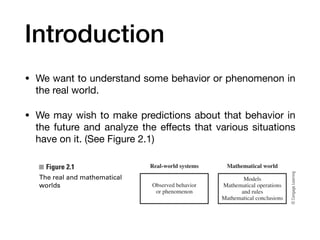
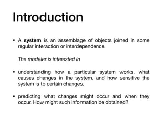
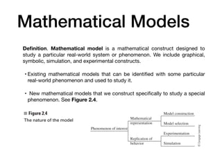
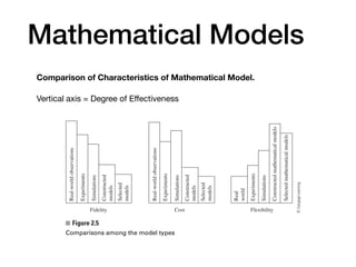
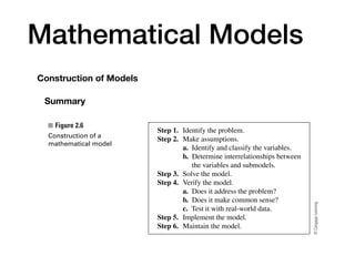
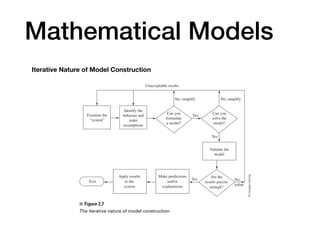
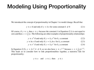
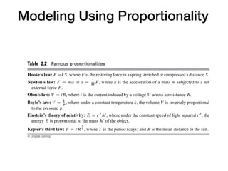
Mathematical
Modeling
Chapter 2.
The Modeling Process, Proportionality, and
Geometric Similarity
Content
• Introduction
• Mathematical Models
• Modeling Using Proportionality
• Modeling Using Geometric Similarity
• Automobile Gasoline Mileage
• Body Weight and Height, Strength and Agility
Introduction
• We want to understand some behavior or phenomenon in
the real world.
• We may wish to make predictions about that behavior in
the future and analyze the e
ff
ects that various situations
have on it. (See Figure 2.1)
2
2 Proportionality, and
Geometric Similarity
Introduction
In Chapter 1 we presented graphical models representing population size, drug
in the bloodstream, various financial investments, and the distribution of cars
cities for a rental company. Now we examine more closely the process of
modeling. To gain an understanding of the processes involved in mathematic
consider the two worlds depicted in Figure 2.1. Suppose we want to unde
behavior or phenomenon in the real world. We may wish to make predictio
behavior in the future and analyze the effects that various situations have on it.
JFigure 2.1
The real and mathematical
worlds
Real-world systems
Observed behavior
or phenomenon
Mathematical world
Models
Mathematical operations
and rules
Mathematical conclusions
©
Cengage
Learning
For example, when studying the populations of two interacting species,
to know if the species can coexist within their environment or if one species w
dominate and drive the other to extinction. In the case of the administration o
Introduction
• A system is an assemblage of objects joined in some
regular interaction or interdependence.
The modeler is interested in
• understanding how a particular system works, what
causes changes in the system, and how sensitive the
system is to certain changes.
• predicting what changes might occur and when they
occur. How might such information be obtained?
Introduction
Goal. Draw conclusions about an observed phenomenon in
the real world.
Two approaches to conclusions about the real world :
Approach 1. One procedure would be to conduct some real-
world behavior trials or experiments and observe their e
ff
ect
on the real-world behavior (See Figure 2.2).
Drawback. This approach can be undoable, or too costly, or
too harmful.
Introduction
Giordano-5166 50904_02_ch02_p058-104 January 23, 2013 19:39 59
2.0 Intr
JFigure 2.2
Reaching conclusions about
the behavior of real-world
systems
Real-world
behavior
Real-world
conclusions
Simplification
Interpretation
Trials Analysis
Model
Mathematical
conclusions
Observation
©
Cengage
Learning
for conducting even a single experiment, such as determining the level of
which a drug proves to be fatal or studying the radiation effects of a fail
power plant near a major population area. Or we may not be willing to
single experimental failure, such as when investigating different designs f
for a spacecraft carrying astronauts. Moreover, it may not even be possib
Introduction
Approach 2. Use mathematical modeling (See Figure 2.3).
• We conduct the following rough modeling procedure:
1.Through observation, identify the primary factors involved in
the real-world behavior, possibly making simpli
fi
cations.
2. Conjecture tentative relationships among the factors.
3. Apply mathematical analysis to the resultant model.
4. Interpret mathematical conclusions in terms of the real-
world problem.
Introduction
Giordano-5166 50904_02_ch02_p058-104 January 23, 2013 19:39 60
60 Chapter 2 The Modeling Process, Proportionality, and Geometric Similarity
JFigure 2.3
The modeling process as
a closed system
Real-world
data
Real-world
explanations
or predictions
Simplification
Interpretation
Verification Analysis
Model
Mathematical
conclusions
©
Cengage
Learning
We portrayed this flow of the modeling process in the introduction
show it again in Figure 2.3 as a closed system. Given some real-world s
sufficient data to formulate a model. Next we analyze the model and re
conclusions about it. Then we interpret the model and make predictions or o
Finally, we test our conclusions about the real-world system against new
Mathematical Models
De
fi
nition. Mathematical model is a mathematical construct designed to
study a particular real-world system or phenomenon. We include graphical,
symbolic, simulation, and experimental constructs.
• Existing mathematical models that can be identi
fi
ed with some particular
real-world phenomenon and used to study it.
• New mathematical models that we construct speci
fi
cally to study a special
phenomenon. See Figure 2.4.
2.1
2.1 Mathematical Models
For our purposes we define a mathematical model as a mathematical construct de
to study a particular real-world system or phenomenon. We include graphical, sym
simulation, and experimental constructs. Mathematical models can be differentiate
ther. There are existing mathematical models that can be identified with some par
real-world phenomenon and used to study it. Then there are those mathematical m
that we construct specifically to study a special phenomenon. Figure 2.4 depicts this
entiation between models. Starting from some real-world phenomenon, we can repre
mathematically by constructing a new model or selecting an existing model. On the
hand, we can replicate the phenomenon experimentally or with some kind of simula
Regarding the question of constructing a mathematical model, a variety of cond
can cause us to abandon hope of achieving any success. The mathematics involve
be so complex and intractable that there is little hope of analyzing or solving the m
thereby defeating its utility.
This complexity can occur, for example, when attempting to use a model give
system of partial differential equations or a system of nonlinear algebraic equations.
problem may be so large (in terms of the number of factors involved) that it is imposs
JFigure 2.4
The nature of the model
Phenomenon of interest
Mathematical
representation
Replication of
behavior
Model construction
Model selection
Experimentation
Simulation
©
Cengage
Learning
Copyright 201 Cengage Learning. All Rights Reserved. May not be copied, scanned, or duplicated, in whole or in part. Due to electronic rights, some third party content may be suppressed from the eB
Editorial review has deemed that any suppressed content does not materially affect the overall learning experience. Cengage Learning reserves the right to remove additional content at any time if subsequen
Mathematical Models
There are three characteristics that a Mathematical
model can possess.
• Fidelity: The preciseness of a model’s representation of
reality
• Costs: The total cost of the modeling process
• Flexibility: The ability to change and control conditions
a
ff
ecting the model as required data are gathered
Mathematical Models
Comparison of Characteristics of Mathematical Model.
Vertical axis = Degree of E
ff
ectiveness
and compare their various capabilities for portraying the real world.
To that end, consider the following properties of a model.
Fidelity: The preciseness of a model’s representation of reality
Costs: The total cost of the modeling process
Flexibility: The ability to change and control conditions affecting the model as required
data are gathered
It is useful to know the degree to which a given model possesses each of these characteristics.
However, since specific models vary greatly, even within the classes identified in Figure 2.4,
the best we can hope for is a comparison of the relative performance between the classes of
models for each of the characteristics. The comparisons are depicted in Figure 2.5, where
the ordinate axis denotes the degree of effectiveness of each class.
Real-world
observations
Experiments
Simulations
Constructed
models
Selected
models
Real-world
observations
Experiments
Simulations
Constructed
models
Selected
models
Real
world
Experiments
Simulations
Constructed
mathematical
models
Selected
mathematical
models
Fidelity Cost Flexibility
©
Cengage
Learning
JFigure 2.5
Comparisons among the model types
opyright 201 Cengage Learning. All Rights Reserved. May not be copied, scanned, or duplicated, in whole or in part. Due to electronic rights, some third party content may be suppressed from the eBook and/or eChapter(s).
al review has deemed that any suppressed content does not materially affect the overall learning experience. Cengage Learning reserves the right to remove additional content at any time if subsequent rights restrictions require it.
Mathematical Models
Construction of Models
Step 1: Identify the problem. What is the problem you would like to explore?
• Typically this is a di
ffi
cult step because in real-life situations no one simply
hands you a mathematical problem to solve.
• Usually you have to sort through large amounts of data and identify some
particular aspect of the situation to study.
• Moreover, it is imperative to be su
ffi
ciently precise (ultimately) in the
formulation of the problem to allow for translation of the verbal statements
describing the problem into mathematical symbols. This translation is
accomplished through the next steps.
• It is important to realize that the answer to the question posed might not lead
directly to a usable problem identi
fi
cation.
Mathematical Models
Construction of Models
Step 2: Make assumptions.
• Generally, we cannot hope to capture in a usable mathematical
model all the factors in
fl
uencing the identi
fi
ed problem.
• The task is simpli
fi
ed by reducing the number of factors under
consideration. Then, relationships among the remaining
variables must be determined.
• Again, by assuming relatively simple relationships, we can
reduce the complexity of the problem.
Mathematical Models
Construction of Models
Step 2: Make assumptions. The assumptions fall into two main activities:
• Classifying the variables. What things in
fl
uence the behavior of the problem
identi
fi
ed in Step 1? List these things as variables. The variables the model seeks to
explain are the dependent variables, and there may be several of these. The
remaining variables are the independent variables. Each variable is classi
fi
ed as
dependent, independent, or neither.
• Determine relationships among variables selected for study. Before we can
hypothesize a relationship among the variables, we generally must make some
additional simpli
fi
cations. The problem may be so complex that we cannot see a
relationship among all the variables initially. In such cases it may be possible to
study submodels. That is, we study one or more of the independent variables
separately. Eventually we will connect the submodels together. Studying various
techniques, such as proportionality, will aid in hypothesizing relationships among
the variables.
Mathematical Models
Construction of Models
Step 3: Solve or interpret the model.
• Now put together all the submodels to see what the model is
telling us.
• In some cases the model may consist of mathematical
equations or inequalities that must be solved to
fi
nd the
information we are seeking.
• Often, a problem statement requires a best solution, or optimal
solution, to the model. Models of this type are discussed later.
Mathematical Models
Construction of Models
Step 4: Verifying the model.
• Before we can use the model, we must test it out.
• There are several questions to ask before designing these tests and
collecting data—a process that can be expensive and time-consuming.
• First, does the model answer the problem identi
fi
ed in Step 1, or did it
stray from the key issue as we constructed the model?
• Second, is the model usable in a practical sense? That is, can we really
gather the data necessary to operate the model?
• Third, does the model make common sense?
Mathematical Models
Construction of Models
Step 5: Implement the model.
• We will want to explain our model in terms that the decision
makers and users can understand if it is ever to be of use to
anyone.
• Furthermore, unless the model is placed in a user-friendly
mode, it will quickly fall into disuse. Expensive computer
programs sometimes su
ff
er such a demise. Often the
inclusion of an additional step to facilitate the collection and
input of the data necessary to operate the model determines
its success or failure.
Mathematical Models
Construction of Models
Step 6: Maintain the model.
• Remember that the model is derived from a speci
fi
c
problem identi
fi
ed in Step 1 and from the
assumptions made in Step 2. Has the original problem
changed in any way, or have some previously
neglected factors become important? Does one of the
submodels need to be adjusted?
Mathematical Models
Construction of Models
Summary
not be too enamored of our work. Like any model, our procedure is an approximation proc
and therefore has its limitations. For example, the procedure seems to consist of disc
steps leading to a usable result, but that is rarely the case in practice. Before offering
alternative procedure that emphasizes the iterative nature of the modeling process, l
discuss the advantages of the methodology depicted in Figure 2.6.
The process shown in Figure 2.6 provides a methodology for progressively focus
on those aspects of the problem we wish to study. Furthermore, it demonstrates a curi
blend of creativity with the scientific method used in the modeling process. The first
steps are more artistic or original in nature. They involve abstracting the essential feature
the problem under study, neglecting any factors judged to be unimportant, and postulat
relationships precise enough to help answer the questions posed by the problem. Howe
these relationships must be simple enough to permit the completion of the remaining ste
JFigure 2.6
Construction of a
mathematical model
Step 1. Identify the problem.
Step 2. Make assumptions.
a. Identify and classify the variables.
b. Determine interrelationships between
the variables and submodels.
Step 3. Solve the model.
Step 4. Verify the model.
a. Does it address the problem?
b. Does it make common sense?
c. Test it with real-world data.
Step 5. Implement the model.
Step 6. Maintain the model.
©
Cengage
Learning
Copyright 201 Cengage Learning. All Rights Reserved. May not be copied, scanned, or duplicated, in whole or in part. Due to electronic rights, some third party content may be suppressed from the eBook a
Editorial review has deemed that any suppressed content does not materially affect the overall learning experience. Cengage Learning reserves the right to remove additional content at any time if subsequent right
Mathematical Models
Construction of Models
Read the text
Giordano-5166 50904_02_ch02_p058-104 January 23, 2013 19:39 65
2.1 Mathematical Models 65
Although these steps admittedly involve a degree of craftsmanship, we will learn some
scientific techniques we can apply to appraise the importance of a particular variable and
the preciseness of an assumed relationship. Nevertheless, when generating numbers in
Steps 3 and 4, remember that the process has been largely inexact and intuitive.
EXAMPLE 1 Vehicular Stopping Distance
Scenario Consider the following rule often given in driver education classes:
Allow one car length for every 10 miles of speed under normal driving conditions, but more
distance in adverse weather or road conditions. One way to accomplish this is to use the 2-
second rule for measuring the correct following distance no matter what your speed. To obtain
that distance, watch the vehicle ahead of you pass some definite point on the highway, like a
tar strip or overpass shadow. Then count to yourself ‘‘one thousand and one, one thousand and
two;’’ that is 2 seconds. If you reach the mark before you finish saying those words, then you are
following too close behind.
The preceding rule is implemented easily enough, but how good is it?
Problem Identification Our ultimate goal is to test this rule and suggest another rule if
it fails. However, the statement of the problem—How good is the rule?—is vague. We need
to be more specific and spell out a problem, or ask a question, whose solution or answer will
help us accomplish our goal while permitting a more exact mathematical analysis. Consider
the following problem statement: Predict the vehicle’s total stopping distance as a function
of its speed.
Mathematical Models
Iterative Nature of Model Construction
Refinement is generally achieved in the opposite way to simplification: We introduce
additional variables, assume more sophisticated relationships among the variables, or expand
the scope of the problem. By simplification and refinement, we determine the generality,
realism, and precision of our model. This process cannot be overemphasized and constitutes
the art of modeling. These ideas are summarized in Table 2.1.
We complete this section by introducing several terms that are useful in describing
models. A model is said to be robust when its conclusions do not depend on the precise
satisfaction of the assumptions. A model is fragile if its conclusions do depend on the
precise satisfaction of some sort of conditions. The term sensitivity refers to the degree of
change in a model’s conclusions as some condition on which they depend is varied; the
greater the change, the more sensitive is the model to that condition.
Unacceptable results
Examine the
“system”
Identify the
behavior and
make
assumptions
Can you
formulate
a model?
No, simplify No, simplify
Yes
Yes
Yes
Can you
solve the
model?
Validate the
model
No,
refine
Are the
results precise
enough?
Make predictions
and/or
explanations
Apply results
to the
system
Exit
©
Cengage
Learning
JFigure 2.7
The iterative nature of model construction
Copyright 201 Cengage Learning. All Rights Reserved. May not be copied, scanned, or duplicated, in whole or in part. Due to electronic rights, some third party content may be suppressed from the eBook and/or eChapter(s).
Editorial review has deemed that any suppressed content does not materially affect the overall learning experience. Cengage Learning reserves the right to remove additional content at any time if subsequent rights restrictions require it.
Mathematical Models
Iterative Nature of Model Construction
5166 50904_02_ch02_p058-104 January 23, 2013 19:39 68
Chapter 2 The Modeling Process, Proportionality, and Geometric Similarity
Table 2.1 The art of mathematical modeling: simplifying or refining the model
as required
Model simplification Model refinement
1. Restrict problem identification.
2. Neglect variables.
3. Conglomerate effects of several variables.
4. Set some variables to be constant.
5. Assume simple (linear) relationships.
6. Incorporate more assumptions.
1. Expand the problem.
2. Consider additional variables.
3. Consider each variable in detail.
4. Allow variation in the variables.
5. Consider nonlinear relationships.
6. Reduce the number of assumptions.
© Cengage Learning
2.1
.1 PROBLEMS
Modeling Using Proportionality
8. Is college a financially sound investment? Income is forfeited for 4 years, and the cost
of college is extremely high. What factors determine the total cost of a college educa-
tion? How would you determine the circumstances necessary for the investment to be
profitable?
2.2
.2 Modeling Using Proportionality
We introduced the concept of proportionality in Chapter 1 to model change. Recall that
y / x if and only if y D kx for some constant k 6D 0 (2.1)
Of course, if y / x, then x / y because the constant k in Equation (2.1) is not equal to
zero and then x D . 1
k
/y. The following are other examples of proportionality relationships:
y / x2
if and only if y D k1x2
for k1 a constant (2.2)
y / ln x if and only if y D k2 ln x for k2 a constant (2.3)
y / ex
if and only if y D k3ex
for k3 a constant (2.4)
In Equation (2.2), y D kx2
; k 6D 0, so we also have x / y1=2
because x D . 1
p
k
/y1=2
.
This leads us to consider how to link proportionalities together, a transitive rule for
proportionality:
y / x and x / z; then y / z
Thus, any variables proportional to the same variables are proportional to one another.
Now let’s explore a geometric interpretation of proportionality. In Equation (2.1),
y D kx yields k D y=x. Thus, k may be interpreted as the tangent of the angle ✓ depicted
Modeling Using Proportionality
Johannes Kepler became director of the Prague Observatory. Kepler had been helping Tycho
Brahe in collecting 13 years of observations on the relative motion of the planet Mars. By
1609, Kepler had formulated his first two laws:
1. Each planet moves along an ellipse with the sun at one focus.
2. For each planet, the line from the sun to the planet sweeps out equal areas in equal
times.
Kepler spent many years verifying these laws and formulating the third law given in
Table 2.2, which relates the orbital periods and mean distances of the planets from the sun.
Table 2.2 Famous proportionalities
Hooke’s law: F DkS, where F is the restoring force in a spring stretched or compressed a distance S.
Newton’s law: F D ma or a D 1
m F , where a is the acceleration of a mass m subjected to a net
external force F .
Ohm’s law: V D iR, where i is the current induced by a voltage V across a resistance R:
Boyle’s law: V D k
p , where under a constant temperature k, the volume V is inversely proportional
to the pressure p.
Einstein’s theory of relativity: E D c2M, where under the constant speed of light squared c2, the
energy E is proportional to the mass M of the object.
Kepler’s third law: T D cR
3
2 , where T is the period (days) and R is the mean distance to the sun.
© Cengage Learning
ght 201 Cengage Learning. All Rights Reserved. May not be copied, scanned, or duplicated, in whole or in part. Due to electronic rights, some third party content may be suppressed from the eBook and/or eChapter(s).
iew has deemed that any suppressed content does not materially affect the overall learning experience. Cengage Learning reserves the right to remove additional content at any time if subsequent rights restrictions require it.

Mathematical modeling Chapter2 model process

  • 1.
    Mathematical Modeling Chapter 2. The ModelingProcess, Proportionality, and Geometric Similarity
  • 2.
    Content • Introduction • MathematicalModels • Modeling Using Proportionality • Modeling Using Geometric Similarity • Automobile Gasoline Mileage • Body Weight and Height, Strength and Agility
  • 3.
    Introduction • We wantto understand some behavior or phenomenon in the real world. • We may wish to make predictions about that behavior in the future and analyze the e ff ects that various situations have on it. (See Figure 2.1) 2 2 Proportionality, and Geometric Similarity Introduction In Chapter 1 we presented graphical models representing population size, drug in the bloodstream, various financial investments, and the distribution of cars cities for a rental company. Now we examine more closely the process of modeling. To gain an understanding of the processes involved in mathematic consider the two worlds depicted in Figure 2.1. Suppose we want to unde behavior or phenomenon in the real world. We may wish to make predictio behavior in the future and analyze the effects that various situations have on it. JFigure 2.1 The real and mathematical worlds Real-world systems Observed behavior or phenomenon Mathematical world Models Mathematical operations and rules Mathematical conclusions © Cengage Learning For example, when studying the populations of two interacting species, to know if the species can coexist within their environment or if one species w dominate and drive the other to extinction. In the case of the administration o
  • 4.
    Introduction • A systemis an assemblage of objects joined in some regular interaction or interdependence. The modeler is interested in • understanding how a particular system works, what causes changes in the system, and how sensitive the system is to certain changes. • predicting what changes might occur and when they occur. How might such information be obtained?
  • 5.
    Introduction Goal. Draw conclusionsabout an observed phenomenon in the real world. Two approaches to conclusions about the real world : Approach 1. One procedure would be to conduct some real- world behavior trials or experiments and observe their e ff ect on the real-world behavior (See Figure 2.2). Drawback. This approach can be undoable, or too costly, or too harmful.
  • 6.
    Introduction Giordano-5166 50904_02_ch02_p058-104 January23, 2013 19:39 59 2.0 Intr JFigure 2.2 Reaching conclusions about the behavior of real-world systems Real-world behavior Real-world conclusions Simplification Interpretation Trials Analysis Model Mathematical conclusions Observation © Cengage Learning for conducting even a single experiment, such as determining the level of which a drug proves to be fatal or studying the radiation effects of a fail power plant near a major population area. Or we may not be willing to single experimental failure, such as when investigating different designs f for a spacecraft carrying astronauts. Moreover, it may not even be possib
  • 7.
    Introduction Approach 2. Usemathematical modeling (See Figure 2.3). • We conduct the following rough modeling procedure: 1.Through observation, identify the primary factors involved in the real-world behavior, possibly making simpli fi cations. 2. Conjecture tentative relationships among the factors. 3. Apply mathematical analysis to the resultant model. 4. Interpret mathematical conclusions in terms of the real- world problem.
  • 8.
    Introduction Giordano-5166 50904_02_ch02_p058-104 January23, 2013 19:39 60 60 Chapter 2 The Modeling Process, Proportionality, and Geometric Similarity JFigure 2.3 The modeling process as a closed system Real-world data Real-world explanations or predictions Simplification Interpretation Verification Analysis Model Mathematical conclusions © Cengage Learning We portrayed this flow of the modeling process in the introduction show it again in Figure 2.3 as a closed system. Given some real-world s sufficient data to formulate a model. Next we analyze the model and re conclusions about it. Then we interpret the model and make predictions or o Finally, we test our conclusions about the real-world system against new
  • 9.
    Mathematical Models De fi nition. Mathematicalmodel is a mathematical construct designed to study a particular real-world system or phenomenon. We include graphical, symbolic, simulation, and experimental constructs. • Existing mathematical models that can be identi fi ed with some particular real-world phenomenon and used to study it. • New mathematical models that we construct speci fi cally to study a special phenomenon. See Figure 2.4. 2.1 2.1 Mathematical Models For our purposes we define a mathematical model as a mathematical construct de to study a particular real-world system or phenomenon. We include graphical, sym simulation, and experimental constructs. Mathematical models can be differentiate ther. There are existing mathematical models that can be identified with some par real-world phenomenon and used to study it. Then there are those mathematical m that we construct specifically to study a special phenomenon. Figure 2.4 depicts this entiation between models. Starting from some real-world phenomenon, we can repre mathematically by constructing a new model or selecting an existing model. On the hand, we can replicate the phenomenon experimentally or with some kind of simula Regarding the question of constructing a mathematical model, a variety of cond can cause us to abandon hope of achieving any success. The mathematics involve be so complex and intractable that there is little hope of analyzing or solving the m thereby defeating its utility. This complexity can occur, for example, when attempting to use a model give system of partial differential equations or a system of nonlinear algebraic equations. problem may be so large (in terms of the number of factors involved) that it is imposs JFigure 2.4 The nature of the model Phenomenon of interest Mathematical representation Replication of behavior Model construction Model selection Experimentation Simulation © Cengage Learning Copyright 201 Cengage Learning. All Rights Reserved. May not be copied, scanned, or duplicated, in whole or in part. Due to electronic rights, some third party content may be suppressed from the eB Editorial review has deemed that any suppressed content does not materially affect the overall learning experience. Cengage Learning reserves the right to remove additional content at any time if subsequen
  • 10.
    Mathematical Models De fi nition. Mathematicalmodel is a mathematical construct designed to study a particular real-world system or phenomenon. We include graphical, symbolic, simulation, and experimental constructs. • Existing mathematical models that can be identi fi ed with some particular real-world phenomenon and used to study it. • New mathematical models that we construct speci fi cally to study a special phenomenon. See Figure 2.4. 2.1 2.1 Mathematical Models For our purposes we define a mathematical model as a mathematical construct de to study a particular real-world system or phenomenon. We include graphical, sym simulation, and experimental constructs. Mathematical models can be differentiate ther. There are existing mathematical models that can be identified with some par real-world phenomenon and used to study it. Then there are those mathematical m that we construct specifically to study a special phenomenon. Figure 2.4 depicts this entiation between models. Starting from some real-world phenomenon, we can repre mathematically by constructing a new model or selecting an existing model. On the hand, we can replicate the phenomenon experimentally or with some kind of simula Regarding the question of constructing a mathematical model, a variety of cond can cause us to abandon hope of achieving any success. The mathematics involve be so complex and intractable that there is little hope of analyzing or solving the m thereby defeating its utility. This complexity can occur, for example, when attempting to use a model give system of partial differential equations or a system of nonlinear algebraic equations. problem may be so large (in terms of the number of factors involved) that it is imposs JFigure 2.4 The nature of the model Phenomenon of interest Mathematical representation Replication of behavior Model construction Model selection Experimentation Simulation © Cengage Learning Copyright 201 Cengage Learning. All Rights Reserved. May not be copied, scanned, or duplicated, in whole or in part. Due to electronic rights, some third party content may be suppressed from the eB Editorial review has deemed that any suppressed content does not materially affect the overall learning experience. Cengage Learning reserves the right to remove additional content at any time if subsequen
  • 11.
    Mathematical Models There arethree characteristics that a Mathematical model can possess. • Fidelity: The preciseness of a model’s representation of reality • Costs: The total cost of the modeling process • Flexibility: The ability to change and control conditions a ff ecting the model as required data are gathered
  • 12.
    Mathematical Models Comparison ofCharacteristics of Mathematical Model. Vertical axis = Degree of E ff ectiveness and compare their various capabilities for portraying the real world. To that end, consider the following properties of a model. Fidelity: The preciseness of a model’s representation of reality Costs: The total cost of the modeling process Flexibility: The ability to change and control conditions affecting the model as required data are gathered It is useful to know the degree to which a given model possesses each of these characteristics. However, since specific models vary greatly, even within the classes identified in Figure 2.4, the best we can hope for is a comparison of the relative performance between the classes of models for each of the characteristics. The comparisons are depicted in Figure 2.5, where the ordinate axis denotes the degree of effectiveness of each class. Real-world observations Experiments Simulations Constructed models Selected models Real-world observations Experiments Simulations Constructed models Selected models Real world Experiments Simulations Constructed mathematical models Selected mathematical models Fidelity Cost Flexibility © Cengage Learning JFigure 2.5 Comparisons among the model types opyright 201 Cengage Learning. All Rights Reserved. May not be copied, scanned, or duplicated, in whole or in part. Due to electronic rights, some third party content may be suppressed from the eBook and/or eChapter(s). al review has deemed that any suppressed content does not materially affect the overall learning experience. Cengage Learning reserves the right to remove additional content at any time if subsequent rights restrictions require it.
  • 13.
    Mathematical Models Construction ofModels Step 1: Identify the problem. What is the problem you would like to explore? • Typically this is a di ffi cult step because in real-life situations no one simply hands you a mathematical problem to solve. • Usually you have to sort through large amounts of data and identify some particular aspect of the situation to study. • Moreover, it is imperative to be su ffi ciently precise (ultimately) in the formulation of the problem to allow for translation of the verbal statements describing the problem into mathematical symbols. This translation is accomplished through the next steps. • It is important to realize that the answer to the question posed might not lead directly to a usable problem identi fi cation.
  • 14.
    Mathematical Models Construction ofModels Step 2: Make assumptions. • Generally, we cannot hope to capture in a usable mathematical model all the factors in fl uencing the identi fi ed problem. • The task is simpli fi ed by reducing the number of factors under consideration. Then, relationships among the remaining variables must be determined. • Again, by assuming relatively simple relationships, we can reduce the complexity of the problem.
  • 15.
    Mathematical Models Construction ofModels Step 2: Make assumptions. The assumptions fall into two main activities: • Classifying the variables. What things in fl uence the behavior of the problem identi fi ed in Step 1? List these things as variables. The variables the model seeks to explain are the dependent variables, and there may be several of these. The remaining variables are the independent variables. Each variable is classi fi ed as dependent, independent, or neither. • Determine relationships among variables selected for study. Before we can hypothesize a relationship among the variables, we generally must make some additional simpli fi cations. The problem may be so complex that we cannot see a relationship among all the variables initially. In such cases it may be possible to study submodels. That is, we study one or more of the independent variables separately. Eventually we will connect the submodels together. Studying various techniques, such as proportionality, will aid in hypothesizing relationships among the variables.
  • 16.
    Mathematical Models Construction ofModels Step 3: Solve or interpret the model. • Now put together all the submodels to see what the model is telling us. • In some cases the model may consist of mathematical equations or inequalities that must be solved to fi nd the information we are seeking. • Often, a problem statement requires a best solution, or optimal solution, to the model. Models of this type are discussed later.
  • 17.
    Mathematical Models Construction ofModels Step 4: Verifying the model. • Before we can use the model, we must test it out. • There are several questions to ask before designing these tests and collecting data—a process that can be expensive and time-consuming. • First, does the model answer the problem identi fi ed in Step 1, or did it stray from the key issue as we constructed the model? • Second, is the model usable in a practical sense? That is, can we really gather the data necessary to operate the model? • Third, does the model make common sense?
  • 18.
    Mathematical Models Construction ofModels Step 5: Implement the model. • We will want to explain our model in terms that the decision makers and users can understand if it is ever to be of use to anyone. • Furthermore, unless the model is placed in a user-friendly mode, it will quickly fall into disuse. Expensive computer programs sometimes su ff er such a demise. Often the inclusion of an additional step to facilitate the collection and input of the data necessary to operate the model determines its success or failure.
  • 19.
    Mathematical Models Construction ofModels Step 6: Maintain the model. • Remember that the model is derived from a speci fi c problem identi fi ed in Step 1 and from the assumptions made in Step 2. Has the original problem changed in any way, or have some previously neglected factors become important? Does one of the submodels need to be adjusted?
  • 20.
    Mathematical Models Construction ofModels Summary not be too enamored of our work. Like any model, our procedure is an approximation proc and therefore has its limitations. For example, the procedure seems to consist of disc steps leading to a usable result, but that is rarely the case in practice. Before offering alternative procedure that emphasizes the iterative nature of the modeling process, l discuss the advantages of the methodology depicted in Figure 2.6. The process shown in Figure 2.6 provides a methodology for progressively focus on those aspects of the problem we wish to study. Furthermore, it demonstrates a curi blend of creativity with the scientific method used in the modeling process. The first steps are more artistic or original in nature. They involve abstracting the essential feature the problem under study, neglecting any factors judged to be unimportant, and postulat relationships precise enough to help answer the questions posed by the problem. Howe these relationships must be simple enough to permit the completion of the remaining ste JFigure 2.6 Construction of a mathematical model Step 1. Identify the problem. Step 2. Make assumptions. a. Identify and classify the variables. b. Determine interrelationships between the variables and submodels. Step 3. Solve the model. Step 4. Verify the model. a. Does it address the problem? b. Does it make common sense? c. Test it with real-world data. Step 5. Implement the model. Step 6. Maintain the model. © Cengage Learning Copyright 201 Cengage Learning. All Rights Reserved. May not be copied, scanned, or duplicated, in whole or in part. Due to electronic rights, some third party content may be suppressed from the eBook a Editorial review has deemed that any suppressed content does not materially affect the overall learning experience. Cengage Learning reserves the right to remove additional content at any time if subsequent right
  • 21.
    Mathematical Models Construction ofModels Read the text Giordano-5166 50904_02_ch02_p058-104 January 23, 2013 19:39 65 2.1 Mathematical Models 65 Although these steps admittedly involve a degree of craftsmanship, we will learn some scientific techniques we can apply to appraise the importance of a particular variable and the preciseness of an assumed relationship. Nevertheless, when generating numbers in Steps 3 and 4, remember that the process has been largely inexact and intuitive. EXAMPLE 1 Vehicular Stopping Distance Scenario Consider the following rule often given in driver education classes: Allow one car length for every 10 miles of speed under normal driving conditions, but more distance in adverse weather or road conditions. One way to accomplish this is to use the 2- second rule for measuring the correct following distance no matter what your speed. To obtain that distance, watch the vehicle ahead of you pass some definite point on the highway, like a tar strip or overpass shadow. Then count to yourself ‘‘one thousand and one, one thousand and two;’’ that is 2 seconds. If you reach the mark before you finish saying those words, then you are following too close behind. The preceding rule is implemented easily enough, but how good is it? Problem Identification Our ultimate goal is to test this rule and suggest another rule if it fails. However, the statement of the problem—How good is the rule?—is vague. We need to be more specific and spell out a problem, or ask a question, whose solution or answer will help us accomplish our goal while permitting a more exact mathematical analysis. Consider the following problem statement: Predict the vehicle’s total stopping distance as a function of its speed.
  • 22.
    Mathematical Models Iterative Natureof Model Construction Refinement is generally achieved in the opposite way to simplification: We introduce additional variables, assume more sophisticated relationships among the variables, or expand the scope of the problem. By simplification and refinement, we determine the generality, realism, and precision of our model. This process cannot be overemphasized and constitutes the art of modeling. These ideas are summarized in Table 2.1. We complete this section by introducing several terms that are useful in describing models. A model is said to be robust when its conclusions do not depend on the precise satisfaction of the assumptions. A model is fragile if its conclusions do depend on the precise satisfaction of some sort of conditions. The term sensitivity refers to the degree of change in a model’s conclusions as some condition on which they depend is varied; the greater the change, the more sensitive is the model to that condition. Unacceptable results Examine the “system” Identify the behavior and make assumptions Can you formulate a model? No, simplify No, simplify Yes Yes Yes Can you solve the model? Validate the model No, refine Are the results precise enough? Make predictions and/or explanations Apply results to the system Exit © Cengage Learning JFigure 2.7 The iterative nature of model construction Copyright 201 Cengage Learning. All Rights Reserved. May not be copied, scanned, or duplicated, in whole or in part. Due to electronic rights, some third party content may be suppressed from the eBook and/or eChapter(s). Editorial review has deemed that any suppressed content does not materially affect the overall learning experience. Cengage Learning reserves the right to remove additional content at any time if subsequent rights restrictions require it.
  • 23.
    Mathematical Models Iterative Natureof Model Construction 5166 50904_02_ch02_p058-104 January 23, 2013 19:39 68 Chapter 2 The Modeling Process, Proportionality, and Geometric Similarity Table 2.1 The art of mathematical modeling: simplifying or refining the model as required Model simplification Model refinement 1. Restrict problem identification. 2. Neglect variables. 3. Conglomerate effects of several variables. 4. Set some variables to be constant. 5. Assume simple (linear) relationships. 6. Incorporate more assumptions. 1. Expand the problem. 2. Consider additional variables. 3. Consider each variable in detail. 4. Allow variation in the variables. 5. Consider nonlinear relationships. 6. Reduce the number of assumptions. © Cengage Learning 2.1 .1 PROBLEMS
  • 24.
    Modeling Using Proportionality 8.Is college a financially sound investment? Income is forfeited for 4 years, and the cost of college is extremely high. What factors determine the total cost of a college educa- tion? How would you determine the circumstances necessary for the investment to be profitable? 2.2 .2 Modeling Using Proportionality We introduced the concept of proportionality in Chapter 1 to model change. Recall that y / x if and only if y D kx for some constant k 6D 0 (2.1) Of course, if y / x, then x / y because the constant k in Equation (2.1) is not equal to zero and then x D . 1 k /y. The following are other examples of proportionality relationships: y / x2 if and only if y D k1x2 for k1 a constant (2.2) y / ln x if and only if y D k2 ln x for k2 a constant (2.3) y / ex if and only if y D k3ex for k3 a constant (2.4) In Equation (2.2), y D kx2 ; k 6D 0, so we also have x / y1=2 because x D . 1 p k /y1=2 . This leads us to consider how to link proportionalities together, a transitive rule for proportionality: y / x and x / z; then y / z Thus, any variables proportional to the same variables are proportional to one another. Now let’s explore a geometric interpretation of proportionality. In Equation (2.1), y D kx yields k D y=x. Thus, k may be interpreted as the tangent of the angle ✓ depicted
  • 25.
    Modeling Using Proportionality JohannesKepler became director of the Prague Observatory. Kepler had been helping Tycho Brahe in collecting 13 years of observations on the relative motion of the planet Mars. By 1609, Kepler had formulated his first two laws: 1. Each planet moves along an ellipse with the sun at one focus. 2. For each planet, the line from the sun to the planet sweeps out equal areas in equal times. Kepler spent many years verifying these laws and formulating the third law given in Table 2.2, which relates the orbital periods and mean distances of the planets from the sun. Table 2.2 Famous proportionalities Hooke’s law: F DkS, where F is the restoring force in a spring stretched or compressed a distance S. Newton’s law: F D ma or a D 1 m F , where a is the acceleration of a mass m subjected to a net external force F . Ohm’s law: V D iR, where i is the current induced by a voltage V across a resistance R: Boyle’s law: V D k p , where under a constant temperature k, the volume V is inversely proportional to the pressure p. Einstein’s theory of relativity: E D c2M, where under the constant speed of light squared c2, the energy E is proportional to the mass M of the object. Kepler’s third law: T D cR 3 2 , where T is the period (days) and R is the mean distance to the sun. © Cengage Learning ght 201 Cengage Learning. All Rights Reserved. May not be copied, scanned, or duplicated, in whole or in part. Due to electronic rights, some third party content may be suppressed from the eBook and/or eChapter(s). iew has deemed that any suppressed content does not materially affect the overall learning experience. Cengage Learning reserves the right to remove additional content at any time if subsequent rights restrictions require it.