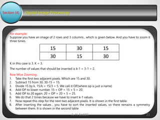
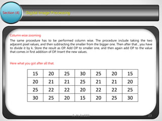
Computer
Science
1
Digital Image Processing
Section (4)
A. H. Seddik 2
Assignment #1
Digital Image Processing
Section (4)
A. H. Seddik 3
Assignment #2
Digital Image Processing
Section (4)
1- Write a MatLab Function that transposes image.
Lab Assignments :-
A. H. Seddik 4
2- Write a MatLab Function that Flips image Vertically.
3- Write a MatLab Function that Obtains negative version of the image.
Digital Image Processing
Section (4)
Cropping Image
A. H. Seddik 5
Digital Image Processing
Section (4)
MatLab Scripts
A. H. Seddik 6
Code in Command Window
Digital Image Processing
Section (4)
MatLab Functions
A. H. Seddik 7
Computer
Science
8
Digital Image Processing
Concept Of Zooming
Section (4)
In this Lecture we are going to introduce the concept of zooming , and the common techniques that
are used to zoom an image.
Zooming
Zooming simply means enlarging a picture in a sense that the details in the image became more
visible and clear. Zooming an image has many wide applications ranging from zooming through a
camera lens , to zoom an image on internet e.t.c.
A. H. Seddik 9
For example
Digital Image Processing
Section (4)
You can zoom something at two different steps:
The first step includes zooming before taking an particular image. This is known as pre processing
zoom. This zoom involves hardware and mechanical movement.
The second step is to zoom once an image has been captured. It is done through many different
algorithms in which we manipulate pixels to zoom in the required portion. We will discuss them in
details next.
Optical Zoom vs digital Zoom
These two types of zoom are supported by the cameras.
A. H. Seddik 10
Optical Zoom:
1. The optical zoom is achieved using the movement of the lens of your camera. An optical zoom is
actually a true zoom.
2. The result of the optical zoom is far better then that of digital zoom. In optical zoom , an
image is magnified by the lens in such a way that the objects in the image appear to be closer
to the camera.
3. In optical zoom the lens is physically extend to zoom or magnify an object.
Digital Image Processing
Section (4)
Digital Zoom:
Digital zoom is basically image processing within a camera. During a digital zoom , the center of the
image is magnified and the edges of the picture got crop out. Due to magnified center , it looks like
that the object is closer to you.
During a digital zoom , the pixels got expand , due to which the quality of the image is compromised.
The same effect of digital zoom can be seen after the image is taken through your computer by using
an image processing toolbox / software, such as Photoshop.
A. H. Seddik 11
The following picture is the result of digital zoom done through
one of the following methods given below in the zooming
methods.
Now since we are learning digital image processing , we will not
focus , on how an image can be zoomed optically using lens or
other stuff. Rather we will focus on the methods, that enable to
zoom a digital image.
Digital Image Processing
Section (4)
Zooming methods:
Although there are many methods that does this job , but we are going to discuss the most
common of them here.
They are listed below:
A. H. Seddik 12
1. Pixel replication or (Nearest neighbor interpolation)
2. Zero order hold method
3. Zooming K times
Each of the methods has its own advantages and disadvantages. We will start by discussing pixel
replication.
Digital Image Processing
Section (4)
Method 1: Pixel replication
Introduction:
A. H. Seddik 13
It is also known as Nearest neighbor interpolation. As its name suggest , in this method , we just
replicate the neighboring pixels. In this method, zooming is nothing but increase amount of pixels.
This algorithm works on the same principle.
Working:
In this method we create new pixels form the already given pixels. Each pixel is replicated in this
method n times row wise and column wise and you got a zoomed image. Its as simple as that.
For example:
if you have an image of 2 rows and 2 columns and you want to zoom it twice or 2 times using pixel
replication, here how it can be done.
For a better understanding , the image has been taken in the form of matrix with the pixel values of
the image.
Digital Image Processing
Section (4)
A. H. Seddik 14
The above image has two rows and two columns, we will first zoom it row wise.
Row wise zooming:
When we zoom it row wise , we will just simple copy the rows pixels to its adjacent new cell.
Here how it would be done.
2
1
4
3
2
2
1
1
4
4
3
3
As you can that in the above matrix , each pixel is replicated twice in the rows.
Digital Image Processing
Section (4)
A. H. Seddik 15
Column wise zooming:
The next step is to replicate each of the pixel column wise, that we will simply copy the column pixel
to its adjacent new column or simply below it.
Here how it would be done.
2
2
1
1
4
4
3
3
2
2
1
1
2
2
1
1
4
4
3
3
4
4
3
3
Digital Image Processing
Section (4)
A. H. Seddik 16
New image size
As it can be seen from the above example , that an original image of 2 rows and 2 columns has been
converted into 4 rows and 4 columns after zooming. That means the new image has a dimensions of
(Original image rows * zooming factor, Original Image cols * zooming factor)
One of the advantage of this zooming technique is , it is very simple. You just have to copy the
pixels and nothing else.
The disadvantage of this technique is that image got zoomed but the output is very blurry. And as
the zooming factor increased , the image got more and more blurred. That would eventually
result in fully blurred image.
Advantage and disadvantage:
Digital Image Processing
Section (4)
Method 2: Zero order hold
Introduction:
A. H. Seddik 17
Zero order hold method is another method of zooming. It is also known as zoom twice. Because it
can only zoom twice. We will see in the below example that why it does that.
Working:
In zero order hold method , we pick two adjacent elements from the rows respectively and then we
add them and divide the result by two, and place their result in between those two elements. We first
do this row wise and then we do this column wise.
For example:
Lets take an image of the dimensions of 2 rows and 2 columns and zoom it twice using zero order
hold.
2
1
4
3
First we will zoom it row wise and then column wise.
Digital Image Processing
Section (4)
A. H. Seddik 18
Row wise zooming:
2
1
1
4
3
3
As we take the first two numbers : (2 + 1) = 3 and then we divide it by 2, we get 1.5 which is
approximated to 1. The same method is applied in the row 2.
Column wise zooming:
2
1
1
3
2
2
4
3
3
We take two adjacent column pixel values which are 1 and 3. We add them and got 4. 4 is then
divided by 2 and we get 2 which is placed in between them. The same method is applied in all the
columns.
Digital Image Processing
Section (4)
A. H. Seddik 19
New image size
As you can see that the dimensions of the new image are 3 x 3 where the original image dimensions
are 2 x 2. So it means that the dimensions of the new image are based on the following formula
(2(number of rows) -1) X (2(number of columns) -1)
One of the advantage of this zooming technique , that it does not create as blurry picture as
compare to the nearest neighbor interpolation method. But it also has a disadvantage that it can only
run on the power of 2. It can be demonstrated here.
Advantage and disadvantage:
Consider the above image of 2 rows and 2 columns. If we have to zoom it 6 times , using zero order
hold method , we can not do it. As the formula shows us this. It could only zoom in the power of 2 -
2,4,8,16,32 and so on.
Even if you try to zoom it, you can not. Because at first when you will zoom it two times, and the result
would be same as shown in the column wise zooming with dimensions equal to 3x3. Then you will
zoom it again and you will get dimensions equal to 5 x 5. Now if you will do it again, you will get
dimensions equal to 9 x 9.
Reason behind twice zooming:
Digital Image Processing
Section (4)
Method 3: K-Times zooming
Introduction:
A. H. Seddik 20
K times is the third zooming method we are going to discuss. It is one of the most perfect zooming
algorithm discussed so far. It caters the challenges of both twice zooming and pixel replication. K in
this zooming algorithm stands for zooming factor.
Working:
It works like this way.
First of all , you have to take two adjacent pixels as you did in the zooming twice. Then you have to
subtract the smaller from the greater one. We call this output (OP).
Divide the output(OP) with the zooming factor(K). Now you have to add the result to the smaller value
and put the result in between those two values.
Add the value OP again to the value you just put and place it again next to the previous putted value.
You have to do it till you place k-1 values in it.
Repeat the same step for all the rows and the columns , and you get a zoomed images.
Digital Image Processing
Section (4)
For example:
A. H. Seddik 21
Suppose you have an image of 2 rows and 3 columns , which is given below. And you have to zoom it
three times.
Row Wise Zooming :
K in this case is 3. K = 3.
The number of values that should be inserted is k-1 = 3-1 = 2.
15
30
15
30
15
30
1. Take the first two adjacent pixels. Which are 15 and 30.
2. Subtract 15 from 30. 30-15 = 15.
3. Divide 15 by k. 15/k = 15/3 = 5. We call it OP.(where op is just a name)
4. Add OP to lower number. 15 + OP = 15 + 5 = 20.
5. Add OP to 20 again. 20 + OP = 20 + 5 = 25.
6. We do that 2 times because we have to insert k-1 values.
7. Now repeat this step for the next two adjacent pixels. It is shown in the first table.
8. After inserting the values , you have to sort the inserted values, so there remains a symmetry
between them. It is shown in the second table
Digital Image Processing
Section (4)
Table 1.
A. H. Seddik 22
15
25
20
30
25
20
15
30
25
20
15
25
20
30
Table 2.
15
20
25
30
25
20
15
30
25
20
15
20
25
30
Digital Image Processing
Section (4)
Column wise zooming
A. H. Seddik 23
The same procedure has to be performed column wise. The procedure include taking the two
adjacent pixel values, and then subtracting the smaller from the bigger one. Then after that , you have
to divide it by k. Store the result as OP. Add OP to smaller one, and then again add OP to the value
that comes in first addition of OP. Insert the new values.
Here what you got after all that.
15
20
25
30
25
20
15
20
21
21
25
21
21
20
25
22
22
20
22
22
25
30
25
20
15
20
25
30
Digital Image Processing
Section (4)
A. H. Seddik 24
New image size
The best way to calculate the formula for the dimensions of a new image is to compare the
dimensions of the original image and the final image. The dimensions of the original image were 2 X
3. And the dimensions of the new image are 4 x 7.The formula thus is:
(K (number of rows -1) + 1) X (K (number of cols -1) + 1)
The one of the clear advantage that k time zooming algorithm has that it is able to compute zoom of
any factor which was the power of pixel replication algorithm , also it gives improved result (less
blurry) which was the power of zero order hold method. So hence It comprises the power of the
two algorithms.
The only difficulty this algorithm has that it has to be sort in the end , which is an additional
step , and thus increases the cost of computation.
Advantage and disadvantage:
Computer
Science
25

Introduction To Digital image Processing

  • 1.
  • 2.
    Digital Image Processing Section(4) A. H. Seddik 2 Assignment #1
  • 3.
    Digital Image Processing Section(4) A. H. Seddik 3 Assignment #2
  • 4.
    Digital Image Processing Section(4) 1- Write a MatLab Function that transposes image. Lab Assignments :- A. H. Seddik 4 2- Write a MatLab Function that Flips image Vertically. 3- Write a MatLab Function that Obtains negative version of the image.
  • 5.
    Digital Image Processing Section(4) Cropping Image A. H. Seddik 5
  • 6.
    Digital Image Processing Section(4) MatLab Scripts A. H. Seddik 6 Code in Command Window
  • 7.
    Digital Image Processing Section(4) MatLab Functions A. H. Seddik 7
  • 8.
  • 9.
    Digital Image Processing ConceptOf Zooming Section (4) In this Lecture we are going to introduce the concept of zooming , and the common techniques that are used to zoom an image. Zooming Zooming simply means enlarging a picture in a sense that the details in the image became more visible and clear. Zooming an image has many wide applications ranging from zooming through a camera lens , to zoom an image on internet e.t.c. A. H. Seddik 9 For example
  • 10.
    Digital Image Processing Section(4) You can zoom something at two different steps: The first step includes zooming before taking an particular image. This is known as pre processing zoom. This zoom involves hardware and mechanical movement. The second step is to zoom once an image has been captured. It is done through many different algorithms in which we manipulate pixels to zoom in the required portion. We will discuss them in details next. Optical Zoom vs digital Zoom These two types of zoom are supported by the cameras. A. H. Seddik 10 Optical Zoom: 1. The optical zoom is achieved using the movement of the lens of your camera. An optical zoom is actually a true zoom. 2. The result of the optical zoom is far better then that of digital zoom. In optical zoom , an image is magnified by the lens in such a way that the objects in the image appear to be closer to the camera. 3. In optical zoom the lens is physically extend to zoom or magnify an object.
  • 11.
    Digital Image Processing Section(4) Digital Zoom: Digital zoom is basically image processing within a camera. During a digital zoom , the center of the image is magnified and the edges of the picture got crop out. Due to magnified center , it looks like that the object is closer to you. During a digital zoom , the pixels got expand , due to which the quality of the image is compromised. The same effect of digital zoom can be seen after the image is taken through your computer by using an image processing toolbox / software, such as Photoshop. A. H. Seddik 11 The following picture is the result of digital zoom done through one of the following methods given below in the zooming methods. Now since we are learning digital image processing , we will not focus , on how an image can be zoomed optically using lens or other stuff. Rather we will focus on the methods, that enable to zoom a digital image.
  • 12.
    Digital Image Processing Section(4) Zooming methods: Although there are many methods that does this job , but we are going to discuss the most common of them here. They are listed below: A. H. Seddik 12 1. Pixel replication or (Nearest neighbor interpolation) 2. Zero order hold method 3. Zooming K times Each of the methods has its own advantages and disadvantages. We will start by discussing pixel replication.
  • 13.
    Digital Image Processing Section(4) Method 1: Pixel replication Introduction: A. H. Seddik 13 It is also known as Nearest neighbor interpolation. As its name suggest , in this method , we just replicate the neighboring pixels. In this method, zooming is nothing but increase amount of pixels. This algorithm works on the same principle. Working: In this method we create new pixels form the already given pixels. Each pixel is replicated in this method n times row wise and column wise and you got a zoomed image. Its as simple as that. For example: if you have an image of 2 rows and 2 columns and you want to zoom it twice or 2 times using pixel replication, here how it can be done. For a better understanding , the image has been taken in the form of matrix with the pixel values of the image.
  • 14.
    Digital Image Processing Section(4) A. H. Seddik 14 The above image has two rows and two columns, we will first zoom it row wise. Row wise zooming: When we zoom it row wise , we will just simple copy the rows pixels to its adjacent new cell. Here how it would be done. 2 1 4 3 2 2 1 1 4 4 3 3 As you can that in the above matrix , each pixel is replicated twice in the rows.
  • 15.
    Digital Image Processing Section(4) A. H. Seddik 15 Column wise zooming: The next step is to replicate each of the pixel column wise, that we will simply copy the column pixel to its adjacent new column or simply below it. Here how it would be done. 2 2 1 1 4 4 3 3 2 2 1 1 2 2 1 1 4 4 3 3 4 4 3 3
  • 16.
    Digital Image Processing Section(4) A. H. Seddik 16 New image size As it can be seen from the above example , that an original image of 2 rows and 2 columns has been converted into 4 rows and 4 columns after zooming. That means the new image has a dimensions of (Original image rows * zooming factor, Original Image cols * zooming factor) One of the advantage of this zooming technique is , it is very simple. You just have to copy the pixels and nothing else. The disadvantage of this technique is that image got zoomed but the output is very blurry. And as the zooming factor increased , the image got more and more blurred. That would eventually result in fully blurred image. Advantage and disadvantage:
  • 17.
    Digital Image Processing Section(4) Method 2: Zero order hold Introduction: A. H. Seddik 17 Zero order hold method is another method of zooming. It is also known as zoom twice. Because it can only zoom twice. We will see in the below example that why it does that. Working: In zero order hold method , we pick two adjacent elements from the rows respectively and then we add them and divide the result by two, and place their result in between those two elements. We first do this row wise and then we do this column wise. For example: Lets take an image of the dimensions of 2 rows and 2 columns and zoom it twice using zero order hold. 2 1 4 3 First we will zoom it row wise and then column wise.
  • 18.
    Digital Image Processing Section(4) A. H. Seddik 18 Row wise zooming: 2 1 1 4 3 3 As we take the first two numbers : (2 + 1) = 3 and then we divide it by 2, we get 1.5 which is approximated to 1. The same method is applied in the row 2. Column wise zooming: 2 1 1 3 2 2 4 3 3 We take two adjacent column pixel values which are 1 and 3. We add them and got 4. 4 is then divided by 2 and we get 2 which is placed in between them. The same method is applied in all the columns.
  • 19.
    Digital Image Processing Section(4) A. H. Seddik 19 New image size As you can see that the dimensions of the new image are 3 x 3 where the original image dimensions are 2 x 2. So it means that the dimensions of the new image are based on the following formula (2(number of rows) -1) X (2(number of columns) -1) One of the advantage of this zooming technique , that it does not create as blurry picture as compare to the nearest neighbor interpolation method. But it also has a disadvantage that it can only run on the power of 2. It can be demonstrated here. Advantage and disadvantage: Consider the above image of 2 rows and 2 columns. If we have to zoom it 6 times , using zero order hold method , we can not do it. As the formula shows us this. It could only zoom in the power of 2 - 2,4,8,16,32 and so on. Even if you try to zoom it, you can not. Because at first when you will zoom it two times, and the result would be same as shown in the column wise zooming with dimensions equal to 3x3. Then you will zoom it again and you will get dimensions equal to 5 x 5. Now if you will do it again, you will get dimensions equal to 9 x 9. Reason behind twice zooming:
  • 20.
    Digital Image Processing Section(4) Method 3: K-Times zooming Introduction: A. H. Seddik 20 K times is the third zooming method we are going to discuss. It is one of the most perfect zooming algorithm discussed so far. It caters the challenges of both twice zooming and pixel replication. K in this zooming algorithm stands for zooming factor. Working: It works like this way. First of all , you have to take two adjacent pixels as you did in the zooming twice. Then you have to subtract the smaller from the greater one. We call this output (OP). Divide the output(OP) with the zooming factor(K). Now you have to add the result to the smaller value and put the result in between those two values. Add the value OP again to the value you just put and place it again next to the previous putted value. You have to do it till you place k-1 values in it. Repeat the same step for all the rows and the columns , and you get a zoomed images.
  • 21.
    Digital Image Processing Section(4) For example: A. H. Seddik 21 Suppose you have an image of 2 rows and 3 columns , which is given below. And you have to zoom it three times. Row Wise Zooming : K in this case is 3. K = 3. The number of values that should be inserted is k-1 = 3-1 = 2. 15 30 15 30 15 30 1. Take the first two adjacent pixels. Which are 15 and 30. 2. Subtract 15 from 30. 30-15 = 15. 3. Divide 15 by k. 15/k = 15/3 = 5. We call it OP.(where op is just a name) 4. Add OP to lower number. 15 + OP = 15 + 5 = 20. 5. Add OP to 20 again. 20 + OP = 20 + 5 = 25. 6. We do that 2 times because we have to insert k-1 values. 7. Now repeat this step for the next two adjacent pixels. It is shown in the first table. 8. After inserting the values , you have to sort the inserted values, so there remains a symmetry between them. It is shown in the second table
  • 22.
    Digital Image Processing Section(4) Table 1. A. H. Seddik 22 15 25 20 30 25 20 15 30 25 20 15 25 20 30 Table 2. 15 20 25 30 25 20 15 30 25 20 15 20 25 30
  • 23.
    Digital Image Processing Section(4) Column wise zooming A. H. Seddik 23 The same procedure has to be performed column wise. The procedure include taking the two adjacent pixel values, and then subtracting the smaller from the bigger one. Then after that , you have to divide it by k. Store the result as OP. Add OP to smaller one, and then again add OP to the value that comes in first addition of OP. Insert the new values. Here what you got after all that. 15 20 25 30 25 20 15 20 21 21 25 21 21 20 25 22 22 20 22 22 25 30 25 20 15 20 25 30
  • 24.
    Digital Image Processing Section(4) A. H. Seddik 24 New image size The best way to calculate the formula for the dimensions of a new image is to compare the dimensions of the original image and the final image. The dimensions of the original image were 2 X 3. And the dimensions of the new image are 4 x 7.The formula thus is: (K (number of rows -1) + 1) X (K (number of cols -1) + 1) The one of the clear advantage that k time zooming algorithm has that it is able to compute zoom of any factor which was the power of pixel replication algorithm , also it gives improved result (less blurry) which was the power of zero order hold method. So hence It comprises the power of the two algorithms. The only difficulty this algorithm has that it has to be sort in the end , which is an additional step , and thus increases the cost of computation. Advantage and disadvantage:
  • 25.