The document outlines projects completed by an intern in machine learning, including handwritten digit recognition using TensorFlow, sentiment analysis on demonetization tweets, and statistical arbitrage detection in Indian stock markets. It discusses the implementation details of each project, such as using TensorFlow for neural networks, data processing with Apache Pig for sentiment analysis, and predictive modeling with neural networks for stock prices. The conclusion emphasizes the challenges in predicting chaotic stock prices and the benefits of simpler models for better generalization.

1. INTERN AS MACHINE LEARNING DEVELOPER
SURAJ KUMAR
CHANDIGARH UNIVERSITY
4th semester

2. PROJECTS
• 1. HANDWRITTEN DIGITS RECOGNITION
• 2. SENTIMENT ANALYSIS ON DEMONITITSATION
• 3. STATISTICAL ARBITRAGE MODEL

3. HANDWRITTEN DIGITS RECOGNITION USING
GOOGLE TENSORFLOW WITH PYTHON
Table of contents:
• What is Tensorflow?
• About the MNIST dataset
• Implementing the Handwritten digits recognition model

4. What is Tensorflow?
• Tensorflow is an open source library created by the Google
Brain Trust for heavy computational work, geared towards
machine learning and deep learning tasks. It is built on C, C++
making its computations very fast while it is available for use
via a Python, C++, Haskell, Java and Go API.
• Tensor: A tensor is any multidimensional array.
• Node: A node is a mathematical computation that is being
worked at the moment.
• A data graph flow essentially maps the flow of information via
the interchange between these two components. Once this
graph is complete, the model is executed and the output is
computed.
• You can learn a lot more from the TENSORFLOW OFFICIAL
DOCUMENT

5. About the MNIST dataset
• To begin our journey with Tensorflow, we will be using the MNIST database
to create an image identifying model based on simple feed forward neural
network with no hidden layers.
• MNIST is a computer vision database consisting of handwritten digits, with
labels identifying the digits. As mentioned earlier, every MNIST data point
has two parts: an image of a handwritten digit and a corresponding label.

6. • We’ll call the images “x” and the labels “y”. Both the training set
and test set contain images and their corresponding labels; for
example, the training images are mnist.train.images and the training
labels are mnist.train.labels.
• Each image is 28 pixels by 28 pixels. We can interpret this as a big
array of numbers. We can flatten this array into a vector of 28×28 =
784 numbers.
• It doesn’t matter how we flatten the array, as long as we’re
consistent between images. From this perspective, the MNIST
images are just a bunch of points in a 784-dimentional vector space.

7. Implementing the Handwritten digits recognition model

8. 1
2
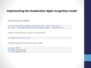
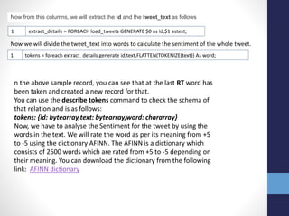
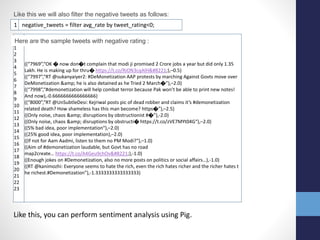
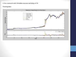
x = tf.placeholder(tf.float32, shape=[None, 784])
y_ = tf.placeholder(tf.float32, shape=[None, 10])
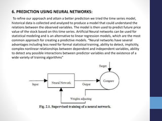
Creating Placeholders
The method tf.placeholder allows us to create variables that act as nodes holding the data. Here,
x is a 2-dimensionall array holding the MNIST images, with none implying the batch size (which
can be of any size) and 784 being a single 28×28 image. y_ is the target output class that
consists of a 2-dimensional array
Creating Variables
1
2
W = tf.Variable(tf.zeros([784, 10]))
b = tf.Variable(tf.zeros([10]))
Initializing the model
Python1 y = tf.nn.softmax(tf.matmul(x,W) + b)
1 cross_entropy = tf.reduce_mean(-tf.reduce_sum(y_ * tf.log(y),
reduction_indices=[1]))
Defining Cost Function
This is the cost function of the model – a cost function is a difference between the predicted
value and the actual value that we are trying to minimize to improve the accuracy of the model.

9. Determining the accuracy of parameters
1
2
correct_prediction = tf.equal(tf.argmax(y,1), tf.argmax(y_,1))
accuracy = tf.reduce_mean(tf.cast(correct_prediction, tf.float32))
1 train_op = tf.train.GradientDescentOptimizer(learning_rate).minimize(cross_entropy)
Implementing Gradient Descent Algorithm
Tensorflow comes pre-loaded with a lot of algorithms, one of them being Gradient Descent. The
gradient descent algorithm starts with an initial value and keeps updating the value till the cost function
reaches the global minimum i.e. the highest level of accuracy.
This is obviously dependant upon the number of iterations being permitted for the model.
Initializing the session
1
2
with tf.Session() as sess:
sess.run(tf.initialize_all_variables())
1
2
for epoch in range(training_epochs):
batch_count = int(mnist.train.num_examples/batch)
for i in range(batch_count):
batch_x, batch_y = mnist.train.next_batch(batch)
Creating batches of data for epochs

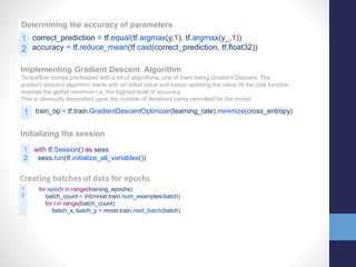
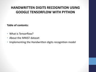
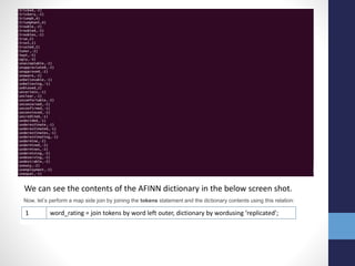
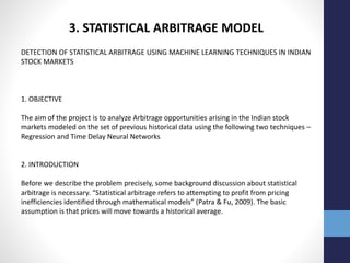
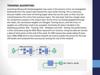
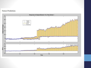
10. Executing the model
1 sess.run([train_op], feed_dict={x: batch_x, y_: batch_y})
Print accuracy of the model
1
2
3
4
if epoch % 2 == 0:
print "Epoch: ", epoch
prit "Accuracy: ", accuracy.eval(feed_dict={x: mnist.test.images, y_:
mnist.test.labels})
print "Model Execution Complete"
Final Note
Creating a deep learning model can be easy and intuitive on Tensorflow. But to
really implement some cool things, you need to have a good grasp on machine
learning principles used in data science.

11. 2. SENTIMENT ANALYSIS ON DEMONITITSATION
Let us find out the views of different people on the demonetization by
analysing the tweets from twitter. Here is the dataset where twitter
tweets are gathered in CSV format.
• You can download the dataset from the below link or ask for data
via mail.
• https://drive.google.com/open?id=0B2nmxAJLHEE8amhpbTl5SzZTQ
Now we will load the data into pig using PigStorage as follows:
1 load_tweets = LOAD ‘/demonetization-tweets.csv’ USING PigStorage(‘,’);

12. Metadata of the tweets are as follows:
• id
• Text (Tweets)
• favorited
• favoriteCount
• replyToSN
• created
• truncated
• replyToSID
• id
• replyToUID
• statusSource
• screenName
• retweetCount
• isRetweet
• retweeted

13. 1 extract_details = FOREACH load_tweets GENERATE $0 as id,$1 astext;
Now from this columns, we will extract the id and the tweet_text as follows
Now we will divide the tweet_text into words to calculate the sentiment of the whole tweet.
1 tokens = foreach extract_details generate id,text,FLATTEN(TOKENIZE(text)) As word;
n the above sample record, you can see that at the last RT word has
been taken and created a new record for that.
You can use the describe tokens command to check the schema of
that relation and is as follows:
tokens: {id: bytearray,text: bytearray,word: chararray}
Now, we have to analyse the Sentiment for the tweet by using the
words in the text. We will rate the word as per its meaning from +5
to -5 using the dictionary AFINN. The AFINN is a dictionary which
consists of 2500 words which are rated from +5 to -5 depending on
their meaning. You can download the dictionary from the following
link: AFINN dictionary

14. We can see the contents of the AFINN dictionary in the below screen shot.
Now, let’s perform a map side join by joining the tokens statement and the dictionary contents using this relation:
1 word_rating = join tokens by word left outer, dictionary by wordusing ‘replicated’;

15. 1 rating = foreach word_rating generate tokens::id as id,tokens::text astext, dictionary::rating as rate;
Now we will extract the id,tweet text and word rating(from the dictionary) by using the
below relation.
We can now see the schema of the relation rating by using the command describe
rating.
rating: {id: bytearray,text: bytearray,rate: int}
In the above statement describe rating we can see that our relation now consists
of id,tweet text andrate(for each word).
1 word_group = group rating by (id,text);
1 avg_rate = foreach word_group generate group, AVG(rating.rate) astweet_rating;
Now we have calculated the Average rating of the tweet using the rating
of each word.
From the above relation, we will get all the tweets i.e., both positive and
negative.

16. 1 positive_tweets = filter avg_rate by tweet_rating>=0;
Here, we can classify the positive tweets by taking the rating of the tweet which can be from 0-
5. We can classify the negative tweets by taking the rating of the tweet from -5 to -1.
We have now successfully performed the Sentiment Analysis on Twitter data using Pig. We
now have the tweets and its rating, so let’s perform an operation to filter out the positive
tweets.
Now we will filter the positive tweets using the below statement:
1
2
3
4
5
6
7
8
9
10
11
12
13
14
15
16
17
18
19
20
21
((“7989”,“RT @rssurjewala: Critical question: Was PayTM informed about #Demonetization edict by PM? It’s clearly
fishy and requires full disclosure &�”),1.0)
((“7990”,“All weddings now need to be approved by RBI… Amazing times #demonetization isn’t that what we are
understanding”),2.0)
((“7993”,“RT @jackerhack: Indore’s collector would like you to shut up about #demonetization. At @internetfreedom
we think that is a problem. https:/�”),2.0)
((“7994”,“@quizderek Post #Dmonetization the result will be totally different.The win is not because of
#demonetization an all knows about it”),4.0)
((“7995”,“@baliramsingh2 So many restrictions. Not easy to avail the facility by anyone. Multiple U-turns by GOI on the
issue. #DeMonetization #RBI”),1.0)
((How long, successful and sustainable will be this strategic game of#DeMonetization against Demons?”),3.0)
((No there r many, we cal them by many names like C#%),2.0)
((Akhilesh=not good,black money is good),3.0)
((And respect their decision,but support oppositio�”),2.0)
((And respect their decision,but support opposition just b‘coz of party“),2.0)
(( the avg indian wants corruptn free india.. So in d name of black money, everybody agrees),1.0)
Here are the sample tweets with positive ratings.

17. 1 negative_tweets = filter avg_rate by tweet_rating<0;
Like this we will also filter the negative tweets as follows:
1
2
3
4
5
6
7
8
9
10
11
12
13
14
15
16
17
18
19
20
21
22
23
((“7969”,“OK � now don�t complain that modi ji promised 2 Crore jobs a year but did only 1.35
Lakh. He is making up for thru� https://t.co/RiON3cqAlH&#8221;),–0.5)
((“7997”,“RT @sukanyaiyer2: #DeMonetization AAP protests by marching Against Govts move over
DeMonetization &amp; he is also detained as he Tried 2 March�”),–2.0)
((“7998”,“#demonetization will help combat terror because Pak won’t be able to print new notes!
And now),-0.6666666666666666)
((“8000”,“RT @UnSubtleDesi: Kejriwal posts pic of dead robber and claims it’s #demonetization
related death? How shameless has this man become? https�”),–2.5)
((Only noise, chaos &amp; disruptions by obstructionist #�”),-2.0)
((Only noise, chaos &amp; disruptions by obstructi� https://t.co/zVE7MYt04G“),–2.0)
((5% bad idea, poor implementation“),–2.0)
((25% good idea, poor implementation),–2.0)
((If not for Aam Aadmi, listen to them no PM Modi?“),–1.0)
((Aim of #demonetization laudable, but Govt has no road
map2create… https://t.co/A4Geu9chOv&#8221;),-1.0)
((Enough jokes on #Demonetization, also no more posts on politics or social affairs…),-1.0)
((RT @kanimozhi: Everyone seems to hate the rich, even the rich hates richer and the richer hates t
he richest.#Demonetization”),-1.3333333333333333)
Here are the sample tweets with negative rating :
Like this, you can perform sentiment analysis using Pig.

18. 3. STATISTICAL ARBITRAGE MODEL
DETECTION OF STATISTICAL ARBITRAGE USING MACHINE LEARNING TECHNIQUES IN INDIAN
STOCK MARKETS
1. OBJECTIVE
The aim of the project is to analyze Arbitrage opportunities arising in the Indian stock
markets modeled on the set of previous historical data using the following two techniques –
Regression and Time Delay Neural Networks
2. INTRODUCTION
Before we describe the problem precisely, some background discussion about statistical
arbitrage is necessary. “Statistical arbitrage refers to attempting to profit from pricing
inefficiencies identified through mathematical models” (Patra & Fu, 2009). The basic
assumption is that prices will move towards a historical average.

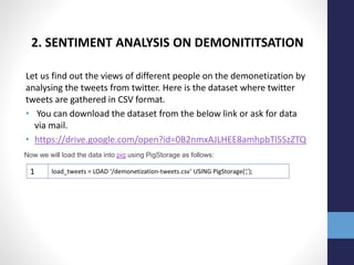
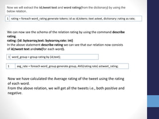
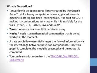
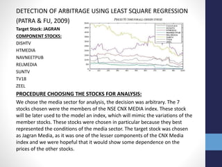
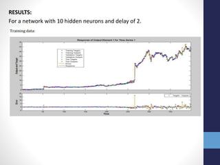
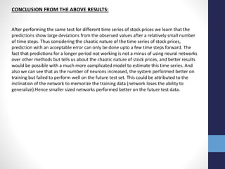
19. 3. WORK DONE PREVIOUSLY:
• Over more than half a century, much empirical research was done on testing the
market efficiency, which can be traced to 1930’s by Alfred Cowles, Many studies have
found that stock prices are at least partially predictable. The method to test the
existence of statistical arbitrage was finally described in the paper “Statistical
arbitrage and tests of market efficiency” [4] by, S.Horgan,
• R.Jarrow, and M. Warachka published in 2002.And an improvement on the paper “An
Improved test for Statistical arbitrage”[5] was published in 2011 by the same team
which forms the basis for this project.
4. MOTIVATION:
• Arbitrage has the effect of causing prices in different markets to converge. [3] “The
speed at which the convergence process occurs usually gives us a measure of the
market efficiency”.
• Hence a thorough analysis of statistical arbitrage opportunities using the advanced
learning techniques is essential in mapping the efficiency of current day Indian
market.

20. DETECTION OF ARBITRAGE USING LEAST SQUARE REGRESSION
(PATRA & FU, 2009)
Target Stock: JAGRAN
COMPONENT STOCKS:
DISHTV
HTMEDIA
NAVNEETPUB
RELMEDIA
SUNTV
TV18
ZEEL
PROCEDURE CHOOSING THE STOCKS FOR ANALYSIS:
We chose the media sector for analysis, the decision was arbitrary. The 7
stocks chosen were the members of the NSE CNX MEDIA index. These stock
will be later used to the model an index, which will mimic the variations of the
member stocks. These stocks were chosen in particular because they best
represented the conditions of the media sector. The target stock was chosen
as Jagran Media, as it was one of the lesser components of the CNX Media
index and we were hopeful that it would show some dependence on the
prices of the other stocks.

21. INITIAL ANALYSIS
1 X-AXIS TIME IN WEEK, Y-AXIS PRICE OF THE STOCKS
MAIN ANALYSIS
2 X- AXIS TIME IN WEEKS, Y-AXIS PRICE OF STOCK

22. 6. PREDICTION USING NEURAL NETWORKS:
To refine our approach and attain a better prediction we tried the time series model,
historical data is collected and analyzed to produce a model that could understand the
relations between the observed variables. The model is then used to predict future price
value of the stock based on this time series. Artificial Neural networks can be used for
statistical modeling and is an alternative to linear regression models, which are the most
common approach for creating a predictive models. “Neural networks have several
advantages including less need for formal statistical training, ability to detect, implicitly,
complex nonlinear relationships between dependent and independent variables, ability
to detect any possible interactions between predictor variables and the existence of a
wide variety of training algorithms”

23. TRAINING ALGORITHM:
Levenberg-Marquardt backpropagation was used, in this process errors are propagated
backwards from the output layer toward the input while training. This is necessary
because hidden units have no training target value that can be used, so they must be
trained based on the errors from previous layers. The only layer that has a target value
for comparison purpose is the output layer. As the errors are backpropagated through
the nodes, the connection weights are changed. Training occurs until the errors in
weights are sufficiently small to be accepted. And lastly the data is divided in the
following quantities 70% - Training, 15% - Validation and 15% - Testing .The performance
is then estimated using the MSE-Mean Squared Error function. Using the data we trained
a data of stock prices at the end of the week, for 400 consecutive weeks (about 8 years
from 2000-2008).And on this trained network we tried to predict the prices for the next
250 weeks and compared the accuracy by varying the size of the network.

24. RESULTS:
For a network with 10 hidden neurons and delay of 2.

28. CONCLUSION FROM THE ABOVE RESULTS:
After performing the same test for different time series of stock prices we learn that the
predictions show large deviations from the observed values after a relatively small number
of time steps. Thus considering the chaotic nature of the time series of stock prices,
prediction with an acceptable error can only be done upto a few time steps forward. The
fact that predictions for a longer period not working is not a minus of using neural networks
over other methods but tells us about the chaotic nature of stock prices, and better results
would be possible with a much more complicated model to estimate this time series. And
also we can see that as the number of neurons increased, the system performed better on
training but failed to perform well on the future test set. This could be attributed to the
inclination of the network to memorize the training data (network loses the ability to
generalize).Hence smaller sized networks performed better on the future test data.

29. 7. FUTURE WORK: To better capture the chaotic nature of the time series
of stock prices,a much more complicated model which is a combination of the
above two methods known of NARX (Nonlinear AutoRegressive with
eXogenous input) can be used. In this method we could use another similar
stock modeled as a time series, along with the data of historical prices of the
same stock.

30. Thanks to Eckovation for giving me opportunity as an
Machine Learning Developer Intern and showing my capabilities in
guidance of such great IIT Educators.
Suraj kumar
Email – sr8804768027@gmail.com
Github-https://github.com/surajrathore007
Chandigarh university
BE-CSE (4th semester)
(Copying or pirating this orignal work is illegal and if found than
legal actions can be taken)