Download to read offline
![Ahmed O. Al- Roubaiy, Saad Hameed Al-Shafaie, Wurood Asaad M
http://www.iaeme.com/IJMET/index.asp 108 editor@iaeme.com
dissimilar metals joining return into the high differences in thermophysical properties between
them as well the easy formation of intermetallic compound at high temperature, which effects
on the mechanical properties of the joints. L. Peng et al. [1]. reported that the brazing metal
consists of (Al, Fe, Si), -Al (Si) and Al of the joint AA1060/AISI 304 by vacuum brazing
technology method using Al-Si filler alloy. J. Yang et al. [2] found that the interface between
the braze seam and the stainless steel contains Fe4Al13 IMC layer of the joint
AA6061/AISI304 using filler alloy of Zn-15Al-xZr.
To achieve a highly qualified joint between aluminum and stainless steel, various welding
processes were investigated. R. Qiu et al. [3] conducted resistance spot welding with a cover
plate of AA5052 to austenitic stainless steel, where reaction products of the joint contain
Fe2Al5 and FeAl3. E. Taban et. al. [4] successfully joined aluminum alloy 6061 to AISI 1018
steel that was investigated with friction stir welding. Intermetallic compounds (IMCs)
appeared, including FeAl and Fe2Al5 in the interfacial reaction layer. C. Dharmendra et al. [5]
suggested the laser welding- brazing process to join zinc coated steel (DP600) with aluminum
alloy (AA6061) using filler wire Zn85-Al15 and various thicknesses of IMC with a difference
in heat input.
S. H. Al- shafaie and S. B. Al-ghazaly [6] investigated improving properties of output
response (elongation, yield stress, and ultimate tensile strength) of welded Al 6061 and Al
7075 aluminum alloy by friction stir welding. K. D. Dwivedi and A. Srivastava [7] found that
Taguchis parameters design approach allows for improving the quality for the joint stainless
steel 304 and C-25 carbon steel using a metal inert gas welding. By Taguchi design, it was
found that the wire feed rate is the first parameter that has the highest effect on the hardness
then current and voltage parameters.
In this paper, a Taguchi method is applied to conduct the experiments and a Grey
Relational Analysis approach is used for development of a second–order polynomial model
and optimize of corrosion rate, shear force and hardness of layer with the time and filler as
input parameters.
2. EXPERIMENTAL WORK
AA 6061 and AISI 304L sheets with dimensions (60x18x1mm) are chosen to produce
dissimilar joints by the brazing process. Two filler alloys AlSi12 and AlSi10Cu4 are applied
as a paste form. The chemical compositions of base alloys and filler alloys are listed in
Table1.
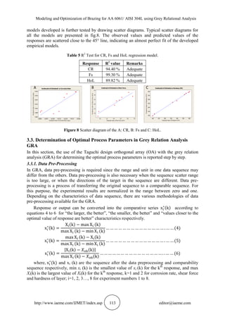
Table 1 Chemical composition of alloys (wt %) [8][9][10]
Alloy % C Cr Si Mn P Mo Ni Al Cu Fe Mg Ti Zn
AISI304L
0.02
5
18.93 0.41 1.42 0.055 0.053 7.85 0.001 0.164 Bal
˗ ˗ ˗
AISI304L
(Standard)[8]
≤
0.03
18-20 ≤ 1.00 ≤ 2.00 ≤ 0.045 - 8-11 - - Bal
AA6061 ˗ 0.11 0.91 0.23 ˗ ˗ 0.06 96.78 0.14 0.57 0.99 0.12 0.08
AA 6061
(Standard)[9]
0.04-
0.35
0.4-0.8
0.15%
96 0.15-0.4 0.7 0.8-1.2 0.15 0.25
AlSi12 ˗ ˗ 11.9 0.01 ˗ ˗ ˗ Bal. <0.01 o.14 0.01 <0.01 <0.01
AlSi12
Standard[10]
11-13 0.15 Bal. 0.30 0.8 0.01 0.20 0.2
AlSi10Cu4 ˗ ˗ 10 0.02 ˗ ˗ ˗ Bal. 4 0.7 0.02 0.03 0.05
AlSi10Cu4
Standard[10]
9.3-
10.7
0.15 Bal. 3.3-4.7 0.8 0.01 0.1-0.2 0.20](https://image.slidesharecdn.com/ijmet1001011-190227065836/85/Ijmet-10-01_011-2-320.jpg)
![Modeling and Optimization of Brazing for AA 6061/ AISI 304L using Grey Relational Analysis
http://www.iaeme.com/IJMET/index.asp 111 editor@iaeme.com
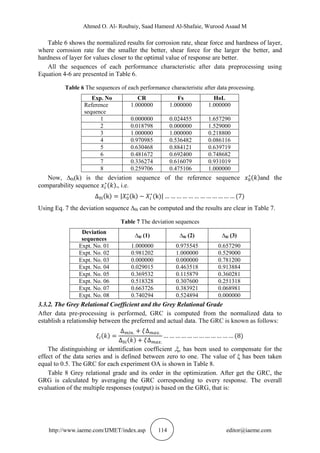
Figure 5 The microstructure for the interfacial joint at 5 min (SEM)
Type of the filler (F) affected on the rate of corrosion through using AlSi12 that improved
the resistance of corrosion due to the presence of (4%Cu) in filler alloy that leads to the
growth of the reaction layer [11].
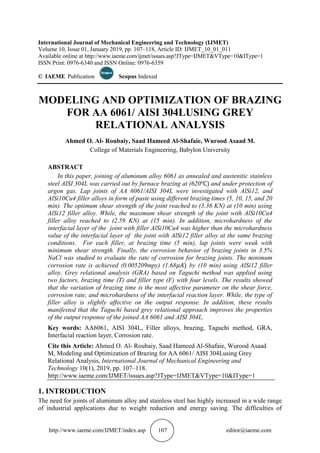
In addition it is seen that as T increases above 5 min the Fs and HoL of brazing AA6061
and 304L increases. While as T increases above 10 min the Fs decreases but the HoL
increases of the joint.
For both filler alloy, when the time of brazing joint increases above 10 min , the Fs of
brazing joint AA6061/ 304L decreases due to the growth of the interfacial layer thickness,
which consists of the intermetallic compounds, Roulin et. al. (1999) found the maximum of
the shear strength joint is (21 MPa) after (10min) brazing time at the brazing temperature
(600 during brazing of aluminum /stainless steel joints using eutectic brazing alloy Al-Si
with different brazing times (5, 10, 20, 40, 60 min )by furnace process [12].
For each brazing time, the Fs of the joint tends to decrease with the filler alloy AlSi10Cu4
due to the 4%Cu in the filler alloy leads to the growth occurrence in the interfacial layer, this
agreement with the present study, Dong et.al. (2012) obtained that the thickness of the
interfacial layer for a joint with AlSi12 less than the thickness of it for the joint with
AlSi10Cu4 [11], see fig. 6.
Figure 6 The effect of brazing time on the thickness of interfacial layer of the joint for both filler
alloys (SEM)
For less than (10 min), at (5 min), the Fs value for the brazing joint reduced due to the
lack of time that is required for a complete wetting between the braze alloy and the base alloy
that led to the deboned of contact area between the faying surfaces.
When the time increases above 10 min, the average hardness of the interfacial layer
increases due to the growth of the interfacial layer with IMCs hardened layer by increasing the
diffusion rate, see fig7.](https://image.slidesharecdn.com/ijmet1001011-190227065836/85/Ijmet-10-01_011-5-320.jpg)
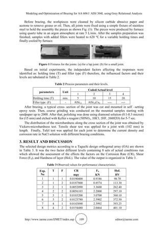
![Ahmed O. Al- Roubaiy, Saad Hameed Al-Shafaie, Wurood Asaad M
http://www.iaeme.com/IJMET/index.asp 112 editor@iaeme.com
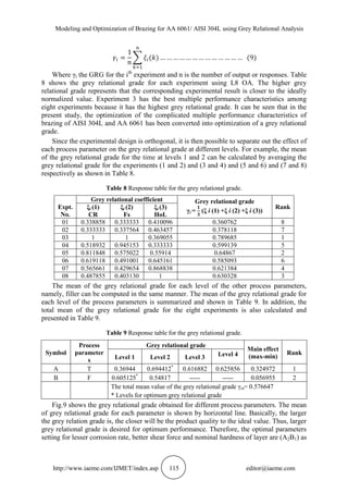
Figure 7 Microstructure of AA 6061/AISI 304L with the different brazing times (SEM) using AlSi12
filler alloy
At the brazing time (5 min), the hardness of the interfacial reaction of the joint is
minimum due to the lack of time that is required for a complete wetting between the braze
alloy and the base that led to to the occurrence deboned.
Besides that, the use of AlSi12 filler alloy led to a fall in the hardness compared with the
using AlSi10Cu4 due to the presence Cu may be distributed in the grain boundaries to form
Al2Cu a brittle intermetallic compound [13,14].
Equations 1 -3 shown below are the predicted regression models for calculating output
(corrosion rate, shear force and hardness of layer). Equations of output are developed with
95% confidence levels.
CR = 0.036376 ˗ 0.022783 T ˗ 0.000589 F + 0.004267 T2
+ 0.000561 T×F.…......... (1)
Fs = ˗ 1.26032 + 3.55876 T ˗ 0.46480 F ˗ 0.62482 T2
˗ 0.01946 T×F......................... (2)
HoL= -173.344 + 280.984 T + 28.025 F -35.719 T2
-4.255 T×F................................. (3)
3.2. Checking the sufficiency of the model
The adequacy of the models so developed is then tested by using the analysis of variance
technique (ANOVA). Using this technique, it can be noted that, as illustrated in Table 4, all
the quadratic regression models significant (0 < p-value < 0.05), except F for all outputs (p-
value > 0.05) and thus all the models adequately represent the experimental data.
Table 4 ANOVA Table for output.
Source DF Seq SS Adj SS Adj MS F P
For CR
T 3 0.000197 0.000197 0.000066 134.34 0.001
F 1 0.000001 0.000001 0.000001 2.72 0.198
Residual Error 3 0.000001 0.000001 0.000000
Total 7 0.000200
For Fs
T 3 4.9075 4.9075 1.6358 15.11 0.026
F 1 0.5273 0.5273 0.5273 4.87 0.114
Residual Error 3 0.3247 0.3247 0.1082
Total 7 5.7595
For HoL
T 3 92174 92779 92174.4 43.82 0.001
F 1 605 605 604.7 0.29 0.615
Residual Error 3 10518 10518 2103.5
Total 7 103297
Another criterion that is commonly used to illustrate the adequacy of a predicted
regression model is the coefficient of determination (R2
). For the models, the calculated R2
values is 94.40%, 99.3% and 89.82 % for Cr, Fs and HoL respectively as shown in Table 5.
These values indicate that the regression models are quite adequate. The validity of regression](https://image.slidesharecdn.com/ijmet1001011-190227065836/85/Ijmet-10-01_011-6-320.jpg)
![Modeling and Optimization of Brazing for AA 6061/ AISI 304L using Grey Relational Analysis
http://www.iaeme.com/IJMET/index.asp 117 editor@iaeme.com
where is the total mean of the grey relational grade is the mean of the grey relational
grade at the optimal level, and q is the number of the process parameters that significantly
affect multiple-performance characteristics.
The obtained process parameters, which give higher grey relational grade, are presented in
Table 11. The predicted CR, Fs, HoL and GRG for the optimal process parameters are
obtained using Equation 10 and also presented in Table 11 which shows the comparison of
the experimental results using the initial (A2B1) and optimal (grey theory prediction design,
A2B1) process parameters. Based on Table 11, the CR decreased from 0.0052090 to
0.0043070 mpy, Fs is accelerated from 3.3600 to 4.1400 KN and the HoL remain
approximately constant at (262.40 ≈ 261.94) HV. The corresponding improvements in CR and
Fs are 17.31%, 18.84 %, respectively. It is clearly shown that the multiple performance
characteristics in the process are greatly improved through this study.
Table 11 Improvements in grey relational grade with optimized process parameters.
Condition
description
Optimal process parameters
Initial process
parameters
Grey theory
Prediction design
Level A2B1 A2B1
CR (mpy) 0.0043070 0.0052090
Fs (KN) 4.1400 3.3600
HoL (HV) 261.94 262.40
GRG 0.710672 0.789685
Improvement in grey relational grade = 0.079013
4. CONCLUSIONS
The shear force of the joint registered an optimum value 3.36KN with AlSi12 at 10 min.
While the maximum shear force of the joint with AlSi10Cu4 reached to 2.59 KN at 15 min.
For the lap joint at (10 min) using AlSi12, the minimum corrosion rate is 0.0052090 mpy.
According to microhardness test, the interfacial layer of the joint with AlSi12 has less
hardness than the hardness of the interfacial layer of joint using AlSi10Cu4.
The optimum value for brazing time 10 min, filler alloy type AlSi12 respectively.
The experiment exhibits the best factors combination and the predicted values were closer to
the observed values.
This approach easily converts the multiple performance characteristics into the GRG, thus
simplifying the analysis.
The results showed that the optimal condition based on the method can offer a better overall
quality.
REFERENCES
[1] Peng Liu, Li Yajiang, Wang Juan, and Guo Jishi (2003) “ Vacuum brazing technology and
microstructure near the interface of Al/18-8 stainless steel”, Materials Research Bulletin,
pp.1493-1499.
[2] Yang Jinlong, Songbai Xue, Peng Xue, Zhaoping Lv, Weimin Long, Guanxing Zhang,
Qingke Zhang, and Peng He (2016) “ Development of Zn-15Al-xZr filler metals for
Brazing 6061 aluminum alloy to stainless steel”, Materials Science and Engineering A,
pp. 425-434.](https://image.slidesharecdn.com/ijmet1001011-190227065836/85/Ijmet-10-01_011-11-320.jpg)
![Ahmed O. Al- Roubaiy, Saad Hameed Al-Shafaie, Wurood Asaad M
http://www.iaeme.com/IJMET/index.asp 118 editor@iaeme.com
[3] Qiu Ranfeng, Chihiro Iwamoto, and Shinobu Satonaka (2008) “ Interfacial microstructure
and strength of steel/aluminum alloy joints welded by resistance spot welding with cover
plate”, Journal of Mterials Processing Technology, pp. 4186-4193.
[4] Taban Emel, Jerry E.Gould, and John C. Lippold (2010) “ Dissimilar friction welding of
606-T6 aluminum and AISI1018 steel: Properties and microstructural characterization”,
Materials and Design, pp. 2305-2311.
[5] Dharmendra C., K.P.Rao, J.Wilden, S.Reich (2011) “ Study on laser welding- brazing of
Zinc coated steel aluminum alloy with a zinc based filler”, Materials Science and
Engineering A, 1497-1503.
[6] Saad Hameed Al-shafaie and Sara bahjet Al-ghazaly (2018) “Optimization of friction stir
welding parameters of Al 6061 and Al 7075 using GRA”,
[7] Kamaleshwar Dhar Dwivedi and Anurag Srivastava ( 2017) “ Parametric Optimization of
MIG Welding for Dissimilar Metals Using Taguchi Design Method” Department of
Mechanical Engineering, S. R. Institute of Management and Technology, A. K. T. U.
Lucknow, Inia, Volume 3.
[8] ASTM Handbook (1989) “Iron and metal products”,vol. 01.01.
[9] ASM Handbook (1990) Properties and Selection: Nonferrous Alloys and Special-Purpose
Materials, American society for Metals, Vol. 2.
[10] Lejeune Road (2007) Specification for Induction Brazing, American Welding Society (
AWS), 2nd
ed.
[11] Dong Honggang, Wenjin Hu, Yuping Duan, Xudong Wang, and Chuang Dong (2012) “
Dissimilar metal joining of aluminum alloy to galvanized steel with Al-Si, Al- Cu, Al-Si-
Cu and Zn-Al filler wires”, Journal of Materials Processing Technology, pp. 458-464.
[12] Roulin M., J.W. Luster, G.Karadeniz and A. Mortensen (1999) “Strength and Structure of
Furnace- Brazed Joints between Aluminum and Stainless Steel”, Welding Research
Supplement.
[13] Kadhim Naief Kadhim and Ahmed H. ( Experimental Study Of Magnetization Effect On
Ground Water Properties).Jordan Journal of Civil Engineering, Volume 12, No. 2, 2018
[14] Lin S. B., J.L.Song, C.L. Yang, C.L. Fan, D. W. Zhang (2010) “ Brazability of dissimilar
metals tungsten inert gas butt welding- brazing between aluminum alloy and stainless steel
with Al-Cu filler alloy”, Materials and Design, pp. 2637-2642.](https://image.slidesharecdn.com/ijmet1001011-190227065836/85/Ijmet-10-01_011-12-320.jpg)

1) The document investigates brazing AA 6061 aluminum alloy to AISI 304L stainless steel using two filler alloys, AlSi12 and AlSi10Cu4, at different brazing times and temperatures. 2) Using a Taguchi design of experiments approach and grey relational analysis, the study found that brazing time had the strongest effect on corrosion rate, shear strength, and hardness of the interface layer, with optimal properties achieved at 10 minutes. 3) Filler alloy type also influenced the results, with AlSi12 generally providing better corrosion resistance due to the presence of copper in the AlSi10Cu4 alloy promoting thicker interfacial layers.