Download as PDF, PPTX
![The New Electric Sector Regime The New Electric Sector Regime
Distributors who demand a relatively high
The weighted average of the prices share of their needs in low price auctions
paid by the regulator for the total will have their profits increased.
energy bought from various
generators will be passed-through to Losses will come to those distributors who
prices. concentrate their demand in the high price
auctions.
Distributors will pay for their energy
in proportion to their declared Distributors are not truly free to allocate
demand in each auction. their demand amongst auctions because
the terms of the contracts being auctioned
monica@ele.puc-rio.br 5
may be incompatible with theirs needs. 6
monica@ele.puc-rio.br
PLD – Settlement Price Simulation
Demand Model
Model
The structure of the demand model is:
Variable Coefficient Standard Error T Statistic Significance
Hydroelectric energy is generally cheaper
Log(C_TOTAL[-1]) 0,772 0,077 10,085 100,0%
but hydro units are not always fully
dispatched since low water levels mean a
Log(PIB[-1]) 0,367 0,122 3,013 98,9%
Log(PR_ENERGIA) -0,189 0,053 -3,564 99,6%
supply risk.
Log(PR_GAS) 0,053 0,017 3,111 99,1%
RACION -0,132 0,022 -6,105 100,0%
Where:
C_total[-1] = consumption in the previous month
C_total[- The ISO ponders the present benefit of
PIB[-1] = GDP in the previous month
PIB[- cheap water use and the future benefits of
PR_ENERGIA = electricity price high level reservoirs, both measured by
PR_GAS = GLP price their opportunity cost in terms of fuel
RACION = dummy variable – rationing period savings in thermoelectric plants.
monica@ele.puc-rio.br 7 monica@ele.puc-rio.br 8](https://image.slidesharecdn.com/icord2007-12729310458563-phpapp01/75/Icord-2007-2-2048.jpg)
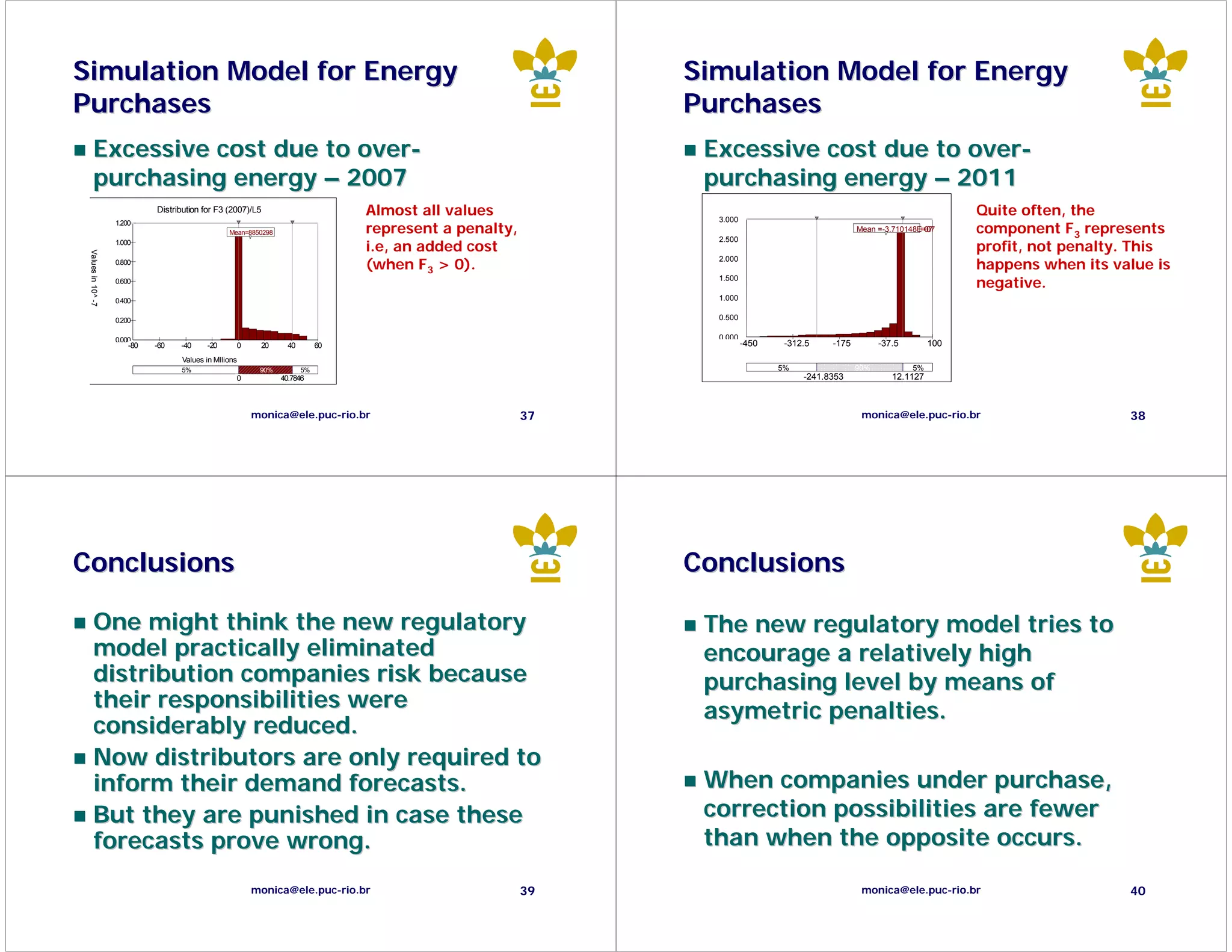

The document discusses decision support methods for energy auctions and risk in the new Brazilian electricity sector regime. It proposes a simulation model to optimize energy purchasing costs for distributors. The model integrates an energy demand forecasting model with simulations of the settlement price (PLD) using hydro dispatch optimization software. It also simulates different percentages of estimated load purchased each year to minimize total costs over multiple years amid demand and PLD uncertainties.


![Ues Commodity Presentation[1]](https://cdn.slidesharecdn.com/ss_thumbnails/uescommoditypresentation1-13388612959775-phpapp02-120604205851-phpapp02-thumbnail.jpg?width=640&height=640&fit=bounds)


