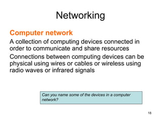
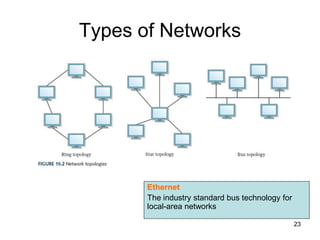
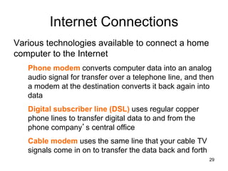
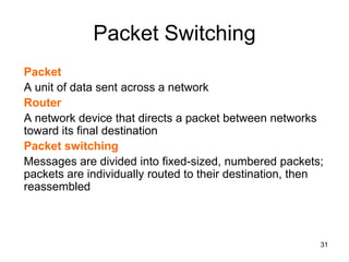
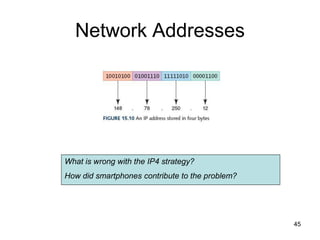
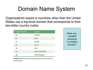
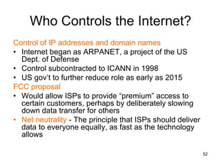
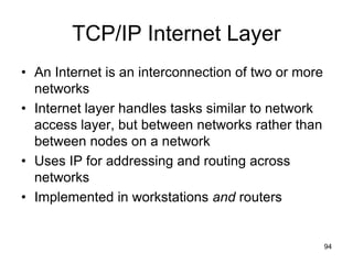
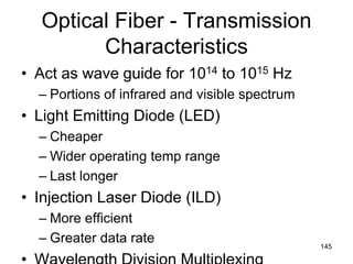
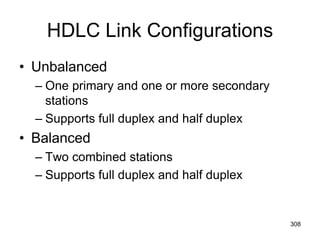
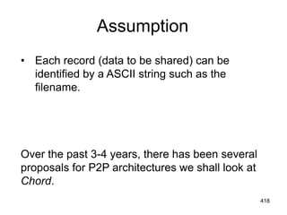
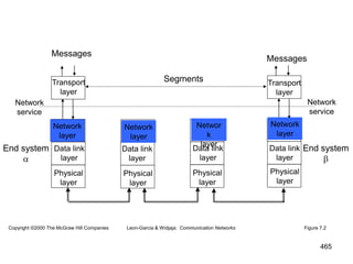
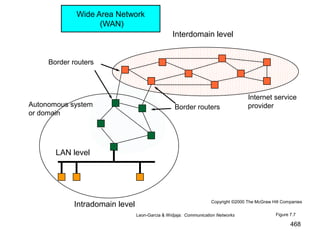
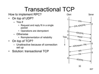
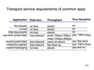
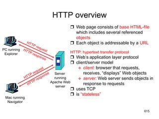
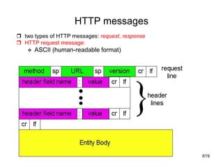
This document provides an introduction to computer networks. It begins with definitions of common network types including local area networks (LANs), metropolitan area networks (MANs), and wide area networks (WANs). It describes common network topologies like bus, star, ring, tree, and mesh. It also discusses network components such as physical media, interconnecting devices, computers, networking software, and applications. The document provides examples of networking applications and protocols like TCP/IP. It introduces concepts like packets, routers, and packet switching. It also discusses open systems, internet connections, network addressing, and the domain name system.

1. COMPUTER NETWORKS
Prepared by:
Dr. Y Mohana Roopa
Mr. P Ravinder
Ms. N M Deepika
Ms. B Jaya Vijaya
INSTITUTE OF AERONAUTICAL ENGINEERING
(Autonomous)
Dundigal, Hyderabad - 500 043
1

2. UNIT-1
2

3. Introduction to Computer Networks
INTRODUCTION TO COMPUTER
NETWORKS
3

4. Computer Networks
Computer network
connects two or more
autonomous computers.
The computers can be
geographically located
anywhere.
Introduction to Computer Networks
4

5. LAN, MAN & WAN
Introduction to Computer Networks
Network in small geographical Area (Room, Building
or a Campus) is called LAN (Local Area Network)
Network in a City is call MAN (Metropolitan Area
Network)
Network spread geographically (Country or across
Globe) is called WAN (Wide Area Network)
5

6. Applications of Networks
Introduction to Computer Networks
Resource Sharing
Hardware (computing resources, disks, printers)
Software (application software)
Information Sharing
Easy accessibility from anywhere (files, databases)
Search Capability (WWW)
Communication
Email
Message broadcast
Remote computing
Distributed processing (GRID Computing) 6

7. Network Topology
The network topology
defines the way in
which computers,
printers, and other
devices are connected.
A network topology
describes the layout of
the wire and devices as
well as the paths used
by data transmissions.
Introduction to Computer Networks
7

8. Bus Topology
Commonly referred to
as a linear bus, all the
devices on a bus
topology are connected
by one single cable.
Introduction to Computer Networks
8

9. Star & Tree Topology
Introduction to Computer Networks
The star topology is the most
commonly used architecture in
Ethernet LANs.
When installed, the star
topology resembles spokes in
a bicycle wheel.
Larger networks use the
extended star topology also
called tree topology. When
used with network devices that
filter frames or packets, like
bridges, switches, and routers,
this topology significantly
reduces the traffic on the wires
by sending packets only to the
wires of the destination host.
9

10. Ring Topology
Introduction to Computer Networks
A frame travels around the ring,
stopping at each node. If a node
wants to transmit data, it adds the
data as well as the destination
address to the frame.
The frame then continues around
the ring until it finds the
destination node, which takes the
data out of the frame.
Single ring – All the devices on
the network share a single cable
Dual ring – The dual ring topology
allows data to be sent in both
directions.
10

11. Mesh Topology
The mesh topology
connects all devices
(nodes) to each other
for redundancy and
fault tolerance.
It is used in WANs to
interconnect LANs and
for mission critical
networks like those
used by banks and
financial institutions.
Implementing the mesh
topology is expensive
and difficult.
Introduction to Computer Networks
11

12. Network Components
Introduction to Computer Networks
Physical Media
Interconnecting Devices
Computers
Networking Software
Applications
12

13. Networking Media
Networking media can
be defined simply as
the means by which
signals (data) are sent
from one computer to
another (either by cable
or wireless means).
Introduction to Computer Networks
13

14. Networking Devices
Introduction to Computer Networks
HUB, Switches, Routers,
Wireless Access Points,
Modems etc.
14

15. Computers: Clients and Servers
In a client/server
network arrangement,
network services are
located in a dedicated
computer whose only
function is to respond
to the requests of
clients.
The server contains the
file, print, application,
security, and other
services in a central
computer that is
continuously available
to respond to client
requests.
Introduction to Computer Networks
15

16. Networking Protocol: TCP/IP
Introduction to Computer Networks
16

17. Applications
E-mail
Searchable Data (Web Sites)
E-Commerce
News Groups
Internet Telephony (VoIP)
Video Conferencing
Chat Groups
Instant Messengers
Internet Radio
Introduction to Computer Networks
17

18. Networking
Computer network
A collection of computing devices connected in
order to communicate and share resources
Connections between computing devices can be
physical using wires or cables or wireless using
radio waves or infrared signals
Can you name some of the devices in a computer
network?
18

19. Networking
Node (host)
Any device on a network
Data transfer rate (bandwidth)
The speed with which data is moved from
one place to another on a network
Why is bandwidth so key?
19

20. Networking
Computer networks have opened up an
entire frontier in the world of computing
called the client/server model
20

21. Networking
Protocol
A set of rules that defines how data is formatted and
processed on a network
File server
A computer dedicated to storing and managing files for
network users
Web server
A computer dedicated to responding to requests for web
pages
P2P model
A decentralized approach that shares resources and
responsibilities among many “peer” computers
21

22. Types of Networks
Local-area network (LAN)
A network that connects a relatively small number
of machines in a relatively close geographical area
Ring topology connects all nodes in a closed loop on
which messages travel in one direction
Star topology centers around one node to which all
others are connected and through which all messages
are sent
Bus topology nodes are connected to a single
communication line that carries messages in both
directions
22

23. Types of Networks
Ethernet
The industry standard bus technology for
local-area networks
23

24. Types of Networks
Wide-area network (WAN)
A network that connects local-area networks over
a potentially large geographic distance
Metropolitan-area network (MAN)
The communication infrastructures that have been
developed in and around large cities
Gateway
One particular set up to handle all communication
going between that LAN and other networks
24

25. Types of Networks
25

26. Types of Networks
Internet
A wide area network that spans the planet
So, who owns the Internet?
26

27. Internet Connections
Wireless network
A network in which devices communicate with
other nodes through a wireless access point
Bluetooth
A technology used for wireless communication
over short distances
27

28. Internet Connections
Internet backbone
A set of high-speed networks that carry Internet
traffic, provided by companies such as AT&T,
Verizon, GTE, British Telecom, and IBM
Internet service provider (ISP)
An organization providing access to the Internet
28

29. Internet Connections
Various technologies available to connect a home
computer to the Internet
Phone modem converts computer data into an analog
audio signal for transfer over a telephone line, and then
a modem at the destination converts it back again into
data
Digital subscriber line (DSL) uses regular copper
phone lines to transfer digital data to and from the
phone company’s central office
Cable modem uses the same line that your cable TV
signals come in on to transfer the data back and forth
29

30. Internet Connections
Broadband
A connection in which transfer speeds are faster
than 768 kilobits per second
– DSL connections and cable modems are broadband
connections
– The speed for downloads (getting data from the
Internet to your home computer) may not be the same
as uploads (sending data from your home computer
to the Internet)
30

31. Packet Switching
Packet
A unit of data sent across a network
Router
A network device that directs a packet between networks
toward its final destination
Packet switching
Messages are divided into fixed-sized, numbered packets;
packets are individually routed to their destination, then
reassembled
31

32. Packet Switching
Take a message, break it into three packets, and
simulate this process
32

33. Open Systems
A logical progression...
Proprietary system
A system that uses technologies kept private by a
particular commercial vendor
Interoperability
The ability of software and hardware on multiple
machines and from multiple commercial vendors to
communicate
Open systems
Systems based on a common model of network
architecture and a suite of protocols used in its
implementation
33

34. Open Systems
Open Systems
Interconnection Reference
Model
A seven-layer logical break
down of network interaction to
facilitate communication
standards
Each layer deals with a
particular aspect of network
communication
34

35. Network Protocols
• Network protocols are layered such that
each one relies on the protocols that
underlie it
• Sometimes referred to as a protocol
stack
35

36. TCP/IP
Transmission Control Protocol (TCP)
Software that breaks messages into packets,
hands them off to the IP software for delivery, and
then orders and reassembles the packets at their
destination
Internet Protocol (IP)
Software that deals with the routing of packets
through the maze of interconnected networks to
their final destination
36

37. TCP/IP
User Datagram Protocol (UDP)
An alternative to TCP that is faster but less reliable
Ping
A program used to test whether a particular
network computer is active and reachable
Traceroute
A program that shows the route a packet takes
across the Internet
37

38. Traceroute in Action
38

39. High-Level Protocols
Other protocols build on TCP/IP protocol suite
Simple Mail Transfer Protocol (SMTP) used to specify
transfer of electronic mail
File Transfer Protocol (FTP) allows a user to transfer
files to and from another computer
Telnet used to log onto one computer from another
Hyper Text Transfer Protocol (http) allows exchange
of Web documents
Which of these have you used?
39

40. High-Level Protocols
Port
A numeric
designation
that
corresponds to
a particular
high-level
protocol
40

41. MIME Types
MIME type
A standard for defining the format of files
that are included as email attachments or on
websites
What does MIME stand for?
Multipurpose Internet Mail Extension
41

42. Firewalls
Firewall
A gateway machine and its software that protects
a network by filtering the traffic it allows
Access control policy
A set of rules established by an organization that
specifies what types of network communication
are permitted and denied
Have your messages ever been
returned undelivered, blocked by a firewall?
42

43. Firewalls
43

44. Network Addresses
Hostname
A name made up of words separated by dots that
uniquely identifies a computer on the Internet
IP address
An address made up of four one-byte numeric
values separated by dots that uniquely identifies a
computer on the Internet
Is there a correspondence between the parts of a hostname
and an IP address?
44

45. Network Addresses
What is wrong with the IP4 strategy?
How did smartphones contribute to the problem?
45

46. Network Addresses
IPv4
The last block was assigned in 2011
IPv6
32 bits organized into 4 groups of 8
FE80:0000:0000:0000:0202:B3FF:FE1E:8329
They work in parallel
46

47. Domain Name System
Host number
The part of the IP address that specifies a
particular host (machine) on the network Yes, but
what is it?
Domain name
The part of a hostname that specifies a specific
organization or group
Top-level domain (TLD)
The last section of a domain name that specifies
the type of organization or its country of origin
47

48. Domain Name System
Domain name system (DNS)
A distributed system for managing hostname
resolution
Domain name server
A computer that attempts to translate a hostname
into an IP address
Domain Squatting
Ransoming domain names
Should the tables containing hostname/IP mappings be
sorted or unsorted? Why?
48

49. Domain Name System
49

50. Domain Name System
Organizations based in countries other than the United
States use a top-level domain that corresponds to their
two-letter country codes
Have you
emailed
someone
in another
country?
50

51. Domain Name System
A very small, random selection of new TLDs that are
available as of mid-2014
51

52. Who Controls the Internet?
Control of IP addresses and domain names
• Internet began as ARPANET, a project of the US
Dept. of Defense
• Control subcontracted to ICANN in 1998
• US gov’t to further reduce role as early as 2015
FCC proposal
• Would allow ISPs to provide “premium” access to
certain customers, perhaps by deliberately slowing
down data transfer for others
• Net neutrality - The principle that ISPs should deliver
data to everyone equally, as fast as the technology
allows
52

53. Cloud Computing
• Public clouds are accessible by any subscriber
• Private clouds are established for a specific group or
organization
• Community clouds are shared among two or more
organizations with the same needs
• Hybrid clouds are some combination of the others
53

54. Ethical Issues
Effects of Social Networking
What are some examples of popular social
networking sites?
Who uses social networking?
What are the benefits and the disadvantages of
using these social networking sites?
Do the benefits of social networking out weigh
the potential costs?
54

55. Brief History of Internet
55

56. Internet Impact
• Check weather
• Buy goods
• Play music
• Find the shortest route
• Give a lecture…
56

57. The Incredible Growth
0
10000000
20000000
30000000
40000000
50000000
60000000
70000000
80000000
Approximate Number of Computers on the Internet
57

58. Brief Internet History
• Batch Environment - 1950s
– No direct interaction between users and their
programs during execution
• Time Sharing - 1960s
– Users were able to interact with the computer and
could share its information processing resources
– Marked the beginning of computer communications
58

59. Brief Internet History (cont.)
Time Sharing:
Dumb terminals connected to
a central computer system
59

60. Brief Internet History (cont.)
• Late 1960s: ARPANET
– ARPA (Advanced Research Projects Agency)
commissioned an experimental computer network
• 1970s:
– Distributed Processing: minicomputers;
• Communication between neighbor processors and
applications via networks
– Growth of ARPANET and Invention of Email
60

61. Brief Internet History (cont.)
• 1980s:
– WAN and LAN
– Prototype Internet
– TCP/IP:Allows different networks to
interconnect
61

62. A LAN Example
B
A
C
D
E
62

63. Internet: a network of networks
The Internet
63

64. Brief Internet History (cont.)
• 1990s: WWW
– HTTP and HTML
– Marc Andreessen: Mosaic (all-in-one solution)
– Commercial traffic allowed ECommerce
64

65. Networking Questions
• Over what medium?
• At what speed?
• How to address computers?
• Which path?
• How to handle (detect & recover) errors?
• What services?
• How to address documents?
• What data format?
65

66. Outline
• Introduction
• OSI Model
• TCP/IP Model
• IPv4 vs. IPv6
66

67. What is a Protocol?
• A standard that allows entities (i.e.
application programs) from different
systems to communicate
• Shared conventions for communicating
information
• Includes syntax, semantics, and timing
67

68. Standardized Protocol
Architectures
• Vendors like standards because they make their
products more marketable
• Customers like standards because they enable
products from different vendors to interoperate
• Two protocol standards are well-known:
– TCP/IP: widely implemented
– OSI: less used, still useful for
modeling/conceptualizing
68

69. Internet Standards
• Email related standards
– IMAP, POP, X.400, SMTP, CMC, MIME, binhex, uuencode
• Web related standards
– http, CGI, html/xml/vrml/sgml
• Internet directory standards
– X.500, LDAP
• Application standards
– http, FTP, telnet, gopher, wais
• Videoconferencing standards
– H.320, H.323, Mpeg-1, Mpeg-2
69

70. *Telecommunication Standards
Organizations
• International Telecommunications Union - Telecommunication
Standardization Sector (ITU-TSS). Formerly called the Consultative
Committee on International Telegraph and Telephone (CCITT)
• International Organization for Standards (ISO). Member of the ITU,
makes technical recommendations about data communications
interfaces.
• American National Standards Institute (ANSI)
• Institute of Electrical and Electronics Engineers (IEEE)
• Internet Engineering Task Force (IETF)
• Electronic Industries Association (EIA)
• National Institute of Standards and Technology (NIST)
• National Exchange Carriers Association (NECA)
• Corporation for Open Systems (COS)
• Electronic Data Interchange -(EDI) of Electronic Data Interchange
for Administration Commerce and Transport (EDIFACT).
70

71. *Internet Engineering Task
Force
A protocol proposed by a vendor
IETF working group study the proposal
IETF issues a request for comment (RFC)
IETF reviews the comments
IETF proposes an improved RFC
The proposed standard becomes a draft
standard if two or more vendors adopt it
The RFC becomes a proposed standard
71

72. What is OSI?
• Developed by the International Organization for
Standardization (ISO) in 1984
• The primary architectural model for intercomputer
communications.
• A conceptual model composed of seven layers, each
specifying particular network functions.
• Describes how information from a software application in
one computer moves through a network medium to a
software application in another computer.
72

73. Why Study OSI?
• Still an excellent model for conceptualizing
and understanding protocol architectures
• Key points:
– Modular
– Hierarchical
– Boundaries between layers=interfaces
73

74. 74

75. Headers and Data
75

76. OSI Lower Layers
• Physical – Layer 1
• Data Link – Layer 2
• Network – Layer 3
76

77. OSI Physical Layer
• Responsible for transmission of bits
• Always implemented through hardware
• Encompasses mechanical, electrical, and
functional interfaces
• e.g. RS-232
77

78. *Physical-layer Implementation
78

79. OSI Data Link Layer
• Responsible for error-free, reliable
transmission of data
• Flow control, error correction
• e.g. HDLC
79

80. OSI Data Link Layer
IEEE has subdivided data link layer into two sub-layers.
80

81. OSI Network Layer
• Responsible for routing of messages
through network
• Concerned with type of switching used
(circuit v. packet)
• Handles routing between networks, as well
as through packet-switching networks
81

82. Network Access Layer
• Concerned with exchange of data between
computer and network
• Includes addressing, routing, prioritizing, etc
• Different networks require different software at
this layer
• Example: X.25 standard for network access
procedures on packet-switching networks
82

83. OSI Upper Layers
• Transport
• Session
• Presentation
• Application
83

84. OSI Transport Layer
• Isolates messages from lower and upper
layers
• Breaks down message size
• Monitors quality of communications
channel
• Selects most efficient communication
service necessary for a given transmission
84

85. Transport Layer
• Concerned with reliable transfer of
information between applications
• Independent of the nature of the
application
• Includes aspects like flow control and error
checking
85

86. OSI Session Layer
• Establishes logical connections between
systems
• Manages log-ons, password exchange,
log-offs
• Terminates connection at end of session
86

87. OSI Presentation Layer
• Provides format and code conversion
services
• Examples
– File conversion from ASCII to EBDIC
– Invoking character sequences to generate
bold, italics, etc on a printer
87

88. OSI Application Layer
• Provides access to network for end-user
• User’s capabilities are determined by what
items are available on this layer
• Logic needed to support various
applications
• Each type of application (file transfer,
remote access) requires different software
on this layer
88

89. Application Viewpoint of a
Network
• Distributed data communications involves
three primary components:
– Networks
– Computers
– Applications
• Three corresponding layers
– Network access layer
– Transport layer
– Application layer
89

90. TCP/IP
• Transmission control Protocol/Internet Protocol
• Developed by DARPA
• No official protocol standard
• Can identify five layers
– Application
– Host-to-Host (transport)
– Internet
– Network Access
– Physical
90

91. An OSI View of TCP/IP
Application
layer
Network
layer
Data Link layer
Physical layer
OSI Model F-D’s Model
Application
(http, telnet, snmp,
smtp, nfs, ftp)
Transport
(TCP, UDP)
Network Access
Physical layer
Internet Model
Internet (IPv4/IPv6)
(HDLC)
91

92. Application
Layer
Transport
Layer
Network
Layer
Data Link
Layer
Physical
Layer
HTTP Request
HTTP
TCP
HTTP
TCP
IP
HTTP
TCP
IP
Ethernet
Sender Receiver
Request
Request
Request
Application
Layer
Transport
Layer
Network
Layer
Data Link
Layer
Physical
Layer
HTTP Request
HTTP
TCP
HTTP
TCP
IP
HTTP
TCP
IP
Ethernet
Request
Request
Request
92

93. TCP/IP Network Access Layer
• Exchange of data between end system and
network
• Address of host and destination
• Prioritization of transmission
• Software at this layer depends on network (e.g.
X.25 vs. Ethernet)
• Segregation means that no other software
needs to be concerned about net specifics
93

94. TCP/IP Internet Layer
• An Internet is an interconnection of two or more
networks
• Internet layer handles tasks similar to network
access layer, but between networks rather than
between nodes on a network
• Uses IP for addressing and routing across
networks
• Implemented in workstations and routers
94

95. TCP/IP Transport Layer
• Also called host-to-host layer
• Reliable exchange of data between
applications
• Uses TCP protocols for transmission
95

96. TCP/IP Application Layer
• Logic needed to support variety of applications
• Separate module supports each type of
application (e.g. file transfer)
– FTP
– HTTP
– Telnet
– News
– SMTP
96

97. *TCP/IP
Ethernet Token Bus Token Ring FDDI
Internet Protocol
ARP
TELNET FTP SMTP DNS SNMP DHCP
Data link
Physical
Network
Transport
Application
Presentation
Session
ICMP
IGMP
RTP
RTCP
Transmission
Control Protocol
User Datagram
Protocol
OSPF
RIP
97

98. TCP & UDP
• Most TCP/IP applications use TCP for transport
layer
• TCP provides a connection (logical association)
between two entities to regulate flow check
errors
• UDP (User Datagram Protocol) does not
maintain a connection, and therefore does not
guarantee delivery, preserve sequences, or
protect against duplication
98

99. Internetworking
• Interconnected networks, usually implies
TCP/IP
• Can appear to users as a single large
network
• The global Internet is the largest example,
but intranets and extranets are also
examples
99

100. Internetworking
100

101. TCP Segment (TCP PDU)
• Source port (16 bits)
• Destination port (16 bits)
• Sequence number (32 bits)
• Acknowledgment number (32 bits)
• Data Offset (4 bits)
• Reserved (6 bits)
• Flags (6 bits) : URG, ACK, PSH, RST, SYN, FIN
• Window (16 bits)
• Checksum (16 bits)
• Urgent Pointer (16 bits)
• Options (variable)
The size of TCP header is 192 bits = 24 byes.
101

102. IPv4 and IPv6
• IP (IPv4) provides for 32-bit source and
destination addresses, using a 192-bit
header
• IPv6 (1996 standard) provides for 128-bit
addresses, using a 320-bit header.
• Migration to IPv6 will be a very slow
process
102

103. *History of IPng Effort
• By the Winter of 1992 the Internet community had developed four separate
proposals for IPng. These were "CNAT", "IP Encaps", "Nimrod", and
"Simple CLNP". By December 1992 three more proposals followed; "The P
Internet Protocol" (PIP), "The Simple Internet Protocol" (SIP) and "TP/IX". In
the Spring of 1992 the "Simple CLNP" evolved into "TCP and UDP with
Bigger Addresses" (TUBA) and "IP Encaps" evolved into "IP Address
Encapsulation" (IPAE).
• By the fall of 1993, IPAE merged with SIP while still maintaining the name
SIP. This group later merged with PIP and the resulting working group
called themselves "Simple Internet Protocol Plus" (SIPP). At about the
same time the TP/IX Working Group changed its name to "Common
Architecture for the Internet" (CATNIP).
• The IPng area directors made a recommendation for an IPng in July of 1994
[RFC 1752].
• The formal name of IPng is IPv6
103

104. Data and Signals
Copyright © The McGraw-Hill Companies, Inc. Permission required for reproduction or display.
3.104

105. 3-4 TRANSMISSION IMPAIRMENT
Signals travel through transmission media, which are not perfect. The imperfection
causes signal impairment. This means that the signal at the beginning of the
medium is not the same as the signal at the end of the medium. What is sent is not
what is received. Three causes of impairment are attenuation, distortion, and noise.
 Attenuation
 Distortion
 Noise
Topics discussed in this section:
105

106. Figure 3.25 Causes of impairment
106

107. Attenuation
• Means loss of energy -> weaker signal
• When a signal travels through a
medium it loses energy overcoming the
resistance of the medium
• Amplifiers are used to compensate for
this loss of energy by amplifying the
signal.
107

108. Measurement of Attenuation
• To show the loss or gain of energy the
unit “decibel” is used.
dB = 10log10P2/P1
P1 - input signal
P2 - output signal
108

109. Figure 3.26 Attenuation
109

110. Suppose a signal travels through a transmission medium and its power is reduced
to one-half. This means that P2 is (1/2)P1. In this case, the attenuation (loss of
power) can be calculated as
Example 3.26
A loss of 3 dB (–3 dB) is equivalent to losing one-half the power.
110

111. A signal travels through an amplifier, and its power is increased 10 times. This
means that P2 = 10P1 . In this case, the amplification (gain of power) can be
calculated as
Example 3.27
111

112. One reason that engineers use the decibel to measure the changes in the strength
of a signal is that decibel numbers can be added (or subtracted) when we are
measuring several points (cascading) instead of just two. In Figure 3.27 a signal
travels from point 1 to point 4. In this case, the decibel value can be calculated as
Example 3.28
112

113. Figure 3.27 Decibels for Example 3.28
113

114. Sometimes the decibel is used to measure signal power in milliwatts. In this case,
it is referred to as dBm and is calculated as dBm = 10 log10 Pm , where Pm is the
power in milliwatts. Calculate the power of a signal with dBm = −30.
Solution
We can calculate the power in the signal as
Example 3.29
114

115. The loss in a cable is usually defined in decibels per kilometer (dB/km). If the
signal at the beginning of a cable with −0.3 dB/km has a power of 2 mW, what is
the power of the signal at 5 km?
Solution
The loss in the cable in decibels is 5 × (−0.3) = −1.5 dB. We can calculate the
power as
Example 3.30
115

116. Distortion
• Means that the signal changes its form or
shape
• Distortion occurs in composite signals
• Each frequency component has its own
propagation speed traveling through a
medium.
• The different components therefore arrive
with different delays at the receiver.
• That means that the signals have different
phases at the receiver than they did at the
source.
116

117. Figure 3.28 Distortion
117

118. Noise
• There are different types of noise
– Thermal - random noise of electrons in the
wire creates an extra signal
– Induced - from motors and appliances,
devices act are transmitter antenna and
medium as receiving antenna.
– Crosstalk - same as above but between
two wires.
– Impulse - Spikes that result from power
lines, lighning, etc.
118

119. Figure 3.29 Noise
119

120. Signal to Noise Ratio (SNR)
• To measure the quality of a system the
SNR is often used. It indicates the
strength of the signal wrt the noise
power in the system.
• It is the ratio between two powers.
• It is usually given in dB and referred to
as SNRdB.
120

121. The power of a signal is 10 mW and the power of the noise is 1 μW; what are the
values of SNR and SNRdB ?
Solution
The values of SNR and SNRdB can be calculated as follows:
Example 3.31
121

122. The values of SNR and SNRdB for a noiseless channel are
Example 3.32
We can never achieve this ratio in real life; it is an ideal.
122

123. Figure 3.30 Two cases of SNR: a high SNR and a low SNR
123

124. Transmission Media
124

125. Overview
• Guided - wire
• Unguided - wireless
• Characteristics and quality determined by
medium and signal
• For guided, the medium is more important
• For unguided, the bandwidth produced by
the antenna is more important
• Key concerns are data rate and distance
125

126. Design Factors
• Bandwidth
– Higher bandwidth gives higher data rate
• Transmission impairments
– Attenuation
• Interference
• Number of receivers
– In guided media
– More receivers (multi-point) introduce more
attenuation
126

127. Electromagnetic Spectrum
127

128. Guided Transmission Media
• Twisted Pair
• Coaxial cable
• Optical fiber
128

129. Transmission Characteristics of
Guided Media
Frequency
Range
Typical
Attenuation
Typical
Delay
Repeater
Spacing
Twisted pair
(with loading)
0 to 3.5 kHz 0.2 dB/km @
1 kHz
50 µs/km 2 km
Twisted pairs
(multi-pair
cables)
0 to 1 MHz 0.7 dB/km @
1 kHz
5 µs/km 2 km
Coaxial cable 0 to 500 MHz 7 dB/km @ 10
MHz
4 µs/km 1 to 9 km
Optical fiber 186 to 370
THz
0.2 to 0.5
dB/km
5 µs/km 40 km
129

130. Twisted Pair
130

131. Twisted Pair - Applications
• Most common medium
• Telephone network
– Between house and local exchange
(subscriber loop)
• Within buildings
– To private branch exchange (PBX)
• For local area networks (LAN)
– 10Mbps or 100Mbps
131

132. Twisted Pair - Pros and Cons
• Cheap
• Easy to work with
• Low data rate
• Short range
132

133. Twisted Pair - Transmission
Characteristics
• Analog
– Amplifiers every 5km to 6km
• Digital
– Use either analog or digital signals
– repeater every 2km or 3km
• Limited distance
• Limited bandwidth (1MHz)
• Limited data rate (100MHz)
• Susceptible to interference and noise 133

134. Near End Crosstalk
• Coupling of signal from one pair to another
• Coupling takes place when transmit signal
entering the link couples back to receiving
pair
• i.e. near transmitted signal is picked up by
near receiving pair
134

135. Unshielded and Shielded TP
• Unshielded Twisted Pair (UTP)
– Ordinary telephone wire
– Cheapest
– Easiest to install
– Suffers from external EM interference
• Shielded Twisted Pair (STP)
– Metal braid or sheathing that reduces
interference
– More expensive
– Harder to handle (thick, heavy)
135

136. UTP Categories
• Cat 3
– up to 16MHz
– Voice grade found in most offices
– Twist length of 7.5 cm to 10 cm
• Cat 4
– up to 20 MHz
• Cat 5
– up to 100MHz
– Commonly pre-installed in new office buildings
– Twist length 0.6 cm to 0.85 cm
• Cat 5E (Enhanced) –see tables
• Cat 6
• Cat 7
136

137. Comparison of Shielded and
Unshielded Twisted Pair
Attenuation (dB per 100 m) Near-end Crosstalk (dB)
Frequency
(MHz)
Category 3
UTP
Category 5
UTP
150-ohm
STP
Category 3
UTP
Category 5
UTP
150-ohm
STP
1 2.6 2.0 1.1 41 62 58
4 5.6 4.1 2.2 32 53 58
16 13.1 8.2 4.4 23 44 50.4
25 — 10.4 6.2 — 41 47.5
100 — 22.0 12.3 — 32 38.5
300 — — 21.4 — — 31.3137

138. Twisted Pair Categories and
Classes
Category 3
Class C
Category 5
Class D
Category
5E
Category 6
Class E
Category 7
Class F
Bandwidth 16 MHz 100 MHz 100 MHz 200 MHz 600 MHz
Cable Type UTP UTP/FTP UTP/FTP UTP/FTP SSTP
Link Cost
(Cat 5 =1)
0.7 1 1.2 1.5 2.2
138

139. Coaxial Cable
139

140. Coaxial Cable Applications
• Most versatile medium
• Television distribution
– Ariel to TV
– Cable TV
• Long distance telephone transmission
– Can carry 10,000 voice calls simultaneously
– Being replaced by fiber optic
• Short distance computer systems links
• Local area networks 140

141. Coaxial Cable - Transmission
Characteristics
• Analog
– Amplifiers every few km
– Closer if higher frequency
– Up to 500MHz
• Digital
– Repeater every 1km
– Closer for higher data rates
141

142. Optical Fiber
142

143. Optical Fiber - Benefits
• Greater capacity
– Data rates of hundreds of Gbps
• Smaller size & weight
• Lower attenuation
• Electromagnetic isolation
• Greater repeater spacing
– 10s of km at least
143

144. Optical Fiber - Applications
• Long-haul trunks
• Metropolitan trunks
• Rural exchange trunks
• Subscriber loops
• LANs
144

145. Optical Fiber - Transmission
Characteristics
• Act as wave guide for 1014 to 1015 Hz
– Portions of infrared and visible spectrum
• Light Emitting Diode (LED)
– Cheaper
– Wider operating temp range
– Last longer
• Injection Laser Diode (ILD)
– More efficient
– Greater data rate 145

146. Optical Fiber Transmission
Modes
146

147. Frequency Utilization for Fiber
Applications
Wavelength (in
vacuum) range
(nm)
Frequency
range (THz)
Band
label
Fiber type Application
820 to 900 366 to 333 Multimode LAN
1280 to 1350 234 to 222 S Single mode Various
1528 to 1561 196 to 192 C Single mode WDM
1561 to 1620 185 to 192 L Single mode WDM
147

148. Attenuation in Guided Media
148

149. Wireless Transmission
Frequencies
• 2GHz to 40GHz
– Microwave
– Highly directional
– Point to point
– Satellite
• 30MHz to 1GHz
– Omnidirectional
– Broadcast radio
• 3 x 1011 to 2 x 1014
– Infrared
– Local
149

150. UNIT II
INTRODUCTION TO DATA
LINK LAYER
150

151. Link layer
our goals:
• understand principles behind link layer
services:
– error detection, correction
– sharing a broadcast channel: multiple access
– link layer addressing
– local area networks: Ethernet, VLANs
• instantiation, implementation of various
link layer technologies
151

152. Link layer, LANs: outline
5.1 introduction, services
5.2 error detection,
correction
5.3 multiple access
protocols
5.4 link-layer addressing
5.5 Ethernet, LANs
5.6 LAN switches
5.7 a day in the life of a
web request
152

153. Link layer: introduction
terminology:
• hosts and routers: nodes
• communication channels that
connect adjacent nodes along
communication path: links
– wired links
– wireless links
– LANs
• layer-2 packet: frame,
encapsulates datagram
data-link layer has responsibility of
transferring datagram from one node
to physically adjacent node over a link
global ISP
153

154. Link layer: context
• datagram transferred by
different link protocols
over different links:
– e.g., Ethernet on first
link, frame relay on
intermediate links,
802.11 on last link
• each link protocol
provides different services
– e.g., may or may not
provide rdt over link
transportation analogy:
• trip from Princeton to Lausanne
– limo: Princeton to JFK
– plane: JFK to Geneva
– train: Geneva to Lausanne
• tourist = datagram
• transport segment =
communication link
• transportation mode = link
layer protocol
• travel agent = routing
algorithm
154

155. Link layer services
• framing, link access:
– encapsulate datagram into frame, adding
header, trailer
– channel access if shared medium
– “MAC” addresses used in frame headers to
identify source, dest
• different from IP address!
• reliable delivery between adjacent nodes
– we learned how to do this already (chapter 3)!
– seldom used on low bit-error link (fiber, some
twisted pair)
– wireless links: high error rates
• Q: why both link-level and end-end reliability?
155

156. • flow control:
– pacing between adjacent sending and receiving nodes
• error detection:
– errors caused by signal attenuation, noise.
– receiver detects presence of errors:
• signals sender for retransmission or drops frame
• error correction:
– receiver identifies and corrects bit error(s) without resorting to
retransmission
• half-duplex and full-duplex
– with half duplex, nodes at both ends of link can transmit, but not
at same time
Link layer services
(more)
156

157. Where is the link layer
implemented?
• in each and every host
• link layer implemented in
“adaptor” (aka network
interface card NIC)
– Ethernet card, 802.11
card
– implements link,
physical layer
• attaches into host’s
system buses
• combination of hardware,
software, firmware
controller
physical
transmission
cpu memory
host
bus
(e.g., PCI)
network adapter
card
application
transport
network
link
link
physical
157

158. Adaptors communicating
• sending side:
– encapsulates datagram
in frame
– adds error checking bits,
rdt, flow control, etc.
• receiving side
– looks for errors, rdt, flow
control, etc
– extracts datagram,
passes to upper layer at
receiving side
controller controller
sending host receiving host
datagram datagram
datagram
frame
158

159. Link layer, LANs: outline
5.1 introduction, services
5.2 error detection,
correction
5.3 multiple access
protocols
5.4 link-layer addressing
5.5 Ethernet, LANs
5.6 LAN switches
5.7 a day in the life of a
web request
159

160. Error detection
EDC= Error Detection and Correction bits (redundancy)
D = Data protected by error checking, may include header fields
• Error detection not 100% reliable!
• protocol may miss some errors, but rarely
• larger EDC field yields better detection and correction
otherwise
160

161. Parity checking
single bit parity:
 detect single bit
errors
two-dimensional bit parity:
 detect and correct single bit errors
161

162. Internet checksum (review)
sender:
• treat segment contents
as sequence of 16-bit
integers
• checksum: addition
(1’s complement sum)
of segment contents
• sender puts checksum
value into UDP
checksum field
receiver:
• compute checksum of
received segment
• check if computed
checksum equals
checksum field value:
– NO - error detected
– YES - no error
detected. But maybe
errors nonetheless?
goal: detect “errors” (e.g., flipped bits) in transmitted packet
(note: used at transport layer only)
162

163. Cyclic redundancy check
• more powerful error-detection coding
• view data bits, D, as a binary number
• choose r+1 bit pattern (generator), G
• goal: choose r CRC bits, R, such that
– <D,R> exactly divisible by G (modulo 2)
– receiver knows G, divides <D,R> by G. If non-zero
remainder: error detected!
– can detect all burst errors less than r+1 bits
• widely used in practice (Ethernet, 802.11 WiFi, ATM)
163

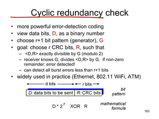
164. CRC example
want:
D.2r XOR R = nG
equivalently:
D.2r = nG XOR R
equivalently:
if we divide D.2r
by G, want
remainder R to
satisfy:
R = remainder[ ]
D.2r
G
164

165. Cyclic Redundancy Check
(CRC)
 Properties of Generator Polynomial
 In general, it is possible to prove that the
following types of errors can be detected by a
G(x) with the stated properties
 All single-bit errors, as long as the xk and x0 terms
have nonzero coefficients.
 All double-bit errors, as long as G(x) has a factor
with at least three terms.
 Any odd number of errors, as long as G(x) contains
the factor (x+1).
 Any “burst” error (i.e., sequence of consecutive
error bits) for which the length of the burst is less
than k bits. (Most burst errors of larger than k bits
can also be detected.)
165

166. Cyclic Redundancy Check
(CRC)
 Six generator polynomials that have become
international standards are:
 CRC-8 = x8+x2+x+1
 CRC-10 = x10+x9+x5+x4+x+1
 CRC-12 = x12+x11+x3+x2+x+1
 CRC-16 = x16+x15+x2+1
 CRC-CCITT = x16+x12+x5+1
 CRC-32 =
x32+x26+x23+x22+x16+x12+x11+x10+x8+x7+x5+x4+x2+
x+1
166

167. Link layer, LANs: outline
5.1 introduction, services
5.2 error detection,
correction
5.3 multiple access
protocols
5.4 link-layer addressing
5.5 Ethernet, LANs
5.6 LAN switches
5.7 a day in the life of a
web request
167

168. Multiple access links, protocols
two types of “links”:
• point-to-point
– PPP for dial-up access
– point-to-point link between Ethernet switch, host
• broadcast (shared wire or medium)
– old-fashioned Ethernet
– upstream HFC
– 802.11 wireless LAN
shared wire (e.g.,
cabled Ethernet)
shared RF
(e.g., 802.11 WiFi)
shared RF
(satellite)
humans at a
cocktail party
(shared air, acoustical)
168

169. Multiple access protocols
• single shared broadcast channel
• two or more simultaneous transmissions by nodes: interference
– collision if node receives two or more signals at the
same time
multiple access protocol
• distributed algorithm that determines how nodes share channel,
i.e., determine when node can transmit
• communication about channel sharing must use channel itself!
– no out-of-band channel for coordination
169

170. An ideal multiple access protocol
given: broadcast channel of rate R bps
desiderata:
1. when one node wants to transmit, it can send
at rate R.
2. when M nodes want to transmit, each can
send at average rate R/M
3. fully decentralized:
• no special node to coordinate transmissions
• no synchronization of clocks, slots
4. simple
170

171. MAC protocols: taxonomy
three broad classes:
• channel partitioning
– divide channel into smaller “pieces” (time slots, frequency,
code)
– allocate piece to node for exclusive use
• random access
– channel not divided, allow collisions
– “recover” from collisions
• “taking turns”
– nodes take turns, but nodes with more to send can take
longer turns
171

172. Channel partitioning MAC protocols:
TDMA
TDMA: time division multiple access
• access to channel in "rounds"
• each station gets fixed length slot
(length = pkt trans time) in each round
• unused slots go idle
• example: 6-station LAN, 1,3,4 have pkt,
slots 2,5,6 idle
1 3 4 1 3 4
6-slot
frame
6-slot
frame
172

173. FDMA: frequency division multiple access
• channel spectrum divided into frequency bands
• each station assigned fixed frequency band
• unused transmission time in frequency bands go idle
• example: 6-station LAN, 1,3,4 have pkt, frequency bands
2,5,6 idle
frequency
bands
FDM cable
Channel partitioning MAC protocols:
FDMA
173

174. Random access protocols
• when node has packet to send
– transmit at full channel data rate R.
– no a priori coordination among nodes
• two or more transmitting nodes ➜
“collision”,
• random access MAC protocol specifies:
– how to detect collisions
– how to recover from collisions (e.g., via
delayed retransmissions)
• examples of random access MAC
protocols:
– slotted ALOHA
– ALOHA
– CSMA, CSMA/CD, CSMA/CA
174

175. Slotted ALOHA
assumptions:
• all frames same size
• time divided into equal
size slots (time to
transmit 1 frame)
• nodes start to transmit
only slot beginning
• nodes are synchronized
• if 2 or more nodes
transmit in slot, all nodes
detect collision
operation:
• when node obtains fresh
frame, transmits in next slot
– if no collision: node can
send new frame in next
slot
– if collision: node
retransmits frame in
each subsequent slot
with prob. p until
success
175

176. Pros:
• single active node can
continuously transmit at
full rate of channel
• highly decentralized:
only slots in nodes need
to be in sync
• simple
Cons:
• collisions, wasting slots
• idle slots
• nodes may be able to
detect collision in less
than time to transmit
packet
• clock synchronization
Slotted ALOHA
1 1 1 1
2
3
2 2
3 3
node 1
node 2
node 3
C C C
S S S
E E E
176

177. • suppose: N nodes with
many frames to send,
each transmits in slot with
probability p
• prob that given node has
success in a slot = p(1-
p)N-1
• prob that any node has a
success = Np(1-p)N-1
• max efficiency: find p*
that maximizes
Np(1-p)N-1
• for many nodes, take
limit of Np*(1-p*)N-1 as N
goes to infinity, gives:
max efficiency = 1/e =
.37
efficiency: long-run
fraction of successful slots
(many nodes, all with many
frames to send)
at best: channel
used for useful
transmissions 37%
of time!
!
Slotted ALOHA: efficiency
177

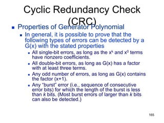
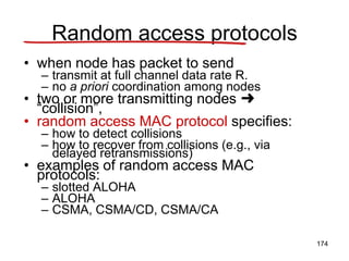
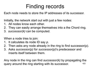
178. Pure (unslotted) ALOHA
• unslotted Aloha: simpler, no synchronization
• when frame first arrives
– transmit immediately
• collision probability increases:
– frame sent at t0 collides with other frames sent
in [t0-1,t0+1]
178

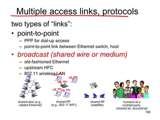
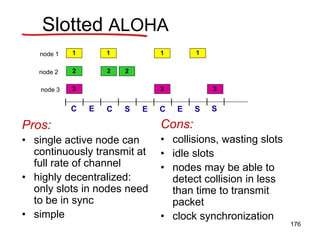
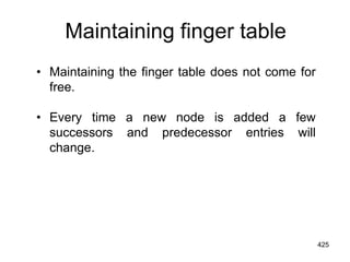
179. Pure ALOHA efficiency
P(success by given node) = P(node transmits) .
P(no other node transmits in [t0-1,t0] .
P(no other node transmits in [t0-1,t0]
= p . (1-p)N-1 . (1-p)N-1
= p . (1-p)2(N-1)
… choosing optimum p and then letting n
= 1/(2e) = .18
even worse than slotted Aloha!
179

180. CSMA (carrier sense multiple
access)
CSMA: listen before transmit:
if channel sensed idle: transmit entire frame
• if channel sensed busy, defer transmission
• human analogy: don’t interrupt others!
180

181. CSMA collisions
• collisions can still
occur: propagation
delay means two
nodes may not hear
each other’s
transmission
• collision: entire packet
transmission time
wasted
– distance & propagation
delay play role in in
determining collision
probability
spatial layout of nodes
181

182. CSMA/CD (collision detection)
CSMA/CD: carrier sensing, deferral as in CSMA
– collisions detected within short time
– colliding transmissions aborted, reducing channel
wastage
• collision detection:
– easy in wired LANs: measure signal strengths,
compare transmitted, received signals
– difficult in wireless LANs: received signal strength
overwhelmed by local transmission strength
• human analogy: the polite conversationalist
182

183. CSMA/CD (collision detection)
spatial layout of nodes
183

184. “Taking turns” MAC protocols
channel partitioning MAC protocols:
– share channel efficiently and fairly at high load
– inefficient at low load: delay in channel access,
1/N bandwidth allocated even if only 1 active
node!
random access MAC protocols
– efficient at low load: single node can fully utilize
channel
– high load: collision overhead
“taking turns” protocols
look for best of both worlds!
184

185. polling:
• master node “invites”
slave nodes to
transmit in turn
• typically used with
“dumb” slave devices
• concerns:
– polling
overhead
– latency
– single point of
failure (master)
master
slaves
poll
data
data
“Taking turns” MAC protocols
185

186. token passing:
 control token passed
from one node to next
sequentially.
 token message
 concerns:
 token overhead
 latency
 single point of failure
(token)
T
data
(nothing
to send)
T
“Taking turns” MAC protocols
186

187. Summary of MAC protocols
• channel partitioning, by time, frequency or code
– Time Division, Frequency Division
• random access (dynamic),
– ALOHA, S-ALOHA, CSMA, CSMA/CD
– carrier sensing: easy in some technologies
(wire), hard in others (wireless)
– CSMA/CD used in Ethernet
– CSMA/CA used in 802.11
• taking turns
– polling from central site, token passing
– bluetooth, FDDI, IBM token ring
187

188. Link layer, LANs: outline
5.1 introduction, services
5.2 error detection,
correction
5.3 multiple access
protocols
5.4 link-layer addressing
5.5 Ethernet, LANs
5.6 LAN switches
5.7 a day in the life of a
web request
188

189. MAC addresses and ARP
• 32-bit IP address:
network-layer address
datagram to destination used to get IP subnet
• MAC (or LAN or physical or Ethernet) address:
function: get frame from one interface to another
physically-connected interface (same network, in IP-
addressing sense)
48 bit MAC address (for most LANs) burned in NIC
ROM, also sometimes software settable
e.g.: 1A-2F-BB-76-09-AD
• Why two addresses for node ??
hexadecimal (base 16) notation
(each “number” represents 4 bits)
189

190. LAN addresses and ARP
each adapter on LAN has unique LAN address
adapter
1A-2F-BB-76-09-AD
58-23-D7-FA-20-B0
0C-C4-11-6F-E3-98
71-65-F7-2B-08-53
LAN
(wired or
wireless)
190

191. LAN addresses (more)
• MAC address allocation administered by IEEE
• manufacturer buys portion of MAC address space
(to assure uniqueness)
• analogy:
– MAC address: like Social Security Number
– IP address: like postal address
• MAC flat address ➜ portability
– can move LAN card from one LAN to another
• IP hierarchical address not portable
– address depends on IP subnet to which node is
attached
191

192. ARP: address resolution protocol
• each IP node (host, router)
on LAN has ARP table
– IP/MAC address
mappings for some
LAN nodes:
< IP address; MAC address;
TTL>
– TTL (Time To Live):
time after which
address mapping
will be forgotten
(typically 20 min)
Question: how to determine
MAC address of B
knowing B’s IP address?
1A-2F-BB-76-09-AD
58-23-D7-FA-20-B0
0C-C4-11-6F-E3-98
71-65-F7-2B-08-53
LAN
137.196.7.23
137.196.7.78
137.196.7.14
137.196.7.88
192

193. ARP protocol: same LAN
• A wants to send datagram
to B
– B’s MAC address not in
A’s ARP table.
• A broadcasts ARP query
packet, containing B's IP
address
– dest MAC address = FF-
FF-FF-FF-FF-FF
– all machines on LAN
receive ARP query
• B receives ARP packet,
replies to A with its (B's)
MAC address
– frame sent to A’s MAC
address (unicast)
• A caches (saves) IP-to-
MAC address pair in its
ARP table until
information becomes
old (times out)
– soft state: information
that times out (goes
away) unless refreshed
• ARP is “plug-and-play”:
– nodes create their ARP
tables without
intervention from net
administrator 193

194. walkthrough: send datagram from A to B via R
– focus on addressing - at both IP (datagram) and MAC layer (frame)
– assume A knows B’s IP address
– assume A knows IP address of first hop router, R (how?)
– assume A knows R’s MAC address (how?)
Addressing: routing to another
LAN
R
1A-23-F9-CD-06-9B
222.222.222.220
111.111.111.110
E6-E9-00-17-BB-4B
CC-49-DE-D0-AB-7D
111.111.111.112
111.111.111.111
74-29-9C-E8-FF-55
A
222.222.222.222
49-BD-D2-C7-56-2A
222.222.222.221
88-B2-2F-54-1A-0F
B
194

195. R
1A-23-F9-CD-06-9B
222.222.222.220
111.111.111.110
E6-E9-00-17-BB-4B
CC-49-DE-D0-AB-7D
111.111.111.112
111.111.111.111
74-29-9C-E8-FF-55
A
222.222.222.222
49-BD-D2-C7-56-2A
222.222.222.221
88-B2-2F-54-1A-0F
B
Addressing: routing to another
LAN
IP
Eth
Phy
IP src: 111.111.111.111
IP dest: 222.222.222.222
 A creates IP datagram with IP source A, destination B
 A creates link-layer frame with R's MAC address as dest, frame
containsA-to-B IP datagram
MAC src: 74-29-9C-E8-FF-55
MAC dest: E6-E9-00-17-BB-4B
195

196. R
1A-23-F9-CD-06-9B
222.222.222.220
111.111.111.110
E6-E9-00-17-BB-4B
CC-49-DE-D0-AB-7D
111.111.111.112
111.111.111.111
74-29-9C-E8-FF-55
A
222.222.222.222
49-BD-D2-C7-56-2A
222.222.222.221
88-B2-2F-54-1A-0F
B
Addressing: routing to another
LAN
IP
Eth
Phy
 frame sent from A to R
IP
Eth
Phy
 frame received at R, datagram removed, passed up to IP
MAC src: 74-29-9C-E8-FF-55
MAC dest: E6-E9-00-17-BB-4B
IP src: 111.111.111.111
IP dest: 222.222.222.222
IP src: 111.111.111.111
IP dest: 222.222.222.222
196

197. R
1A-23-F9-CD-06-9B
222.222.222.220
111.111.111.110
E6-E9-00-17-BB-4B
CC-49-DE-D0-AB-7D
111.111.111.112
111.111.111.111
74-29-9C-E8-FF-55
A
222.222.222.222
49-BD-D2-C7-56-2A
222.222.222.221
88-B2-2F-54-1A-0F
B
Addressing: routing to another
LAN
IP src: 111.111.111.111
IP dest: 222.222.222.222
 R forwards datagram with IP source A, destination B
 R creates link-layer frame with B's MAC address as dest, frame
containsA-to-B IP datagram
MAC src: 1A-23-F9-CD-06-9B
MAC dest: 49-BD-D2-C7-56-2A
IP
Eth
Phy
IP
Eth
Phy
197

198. R
1A-23-F9-CD-06-9B
222.222.222.220
111.111.111.110
E6-E9-00-17-BB-4B
CC-49-DE-D0-AB-7D
111.111.111.112
111.111.111.111
74-29-9C-E8-FF-55
A
222.222.222.222
49-BD-D2-C7-56-2A
222.222.222.221
88-B2-2F-54-1A-0F
B
Addressing: routing to another
LAN
 R forwards datagram with IP source A, destination B
 R creates link-layer frame with B's MAC address as dest, frame
containsA-to-B IP datagram
IP src: 111.111.111.111
IP dest: 222.222.222.222
MAC src: 1A-23-F9-CD-06-9B
MAC dest: 49-BD-D2-C7-56-2A
IP
Eth
Phy
IP
Eth
Phy
198

199. R
1A-23-F9-CD-06-9B
222.222.222.220
111.111.111.110
E6-E9-00-17-BB-4B
CC-49-DE-D0-AB-7D
111.111.111.112
111.111.111.111
74-29-9C-E8-FF-55
A
222.222.222.222
49-BD-D2-C7-56-2A
222.222.222.221
88-B2-2F-54-1A-0F
B
Addressing: routing to another
LAN
 R forwards datagram with IP source A, destination B
 R creates link-layer frame with B's MAC address as dest, frame
containsA-to-B IP datagram
IP src: 111.111.111.111
IP dest: 222.222.222.222
MAC src: 1A-23-F9-CD-06-9B
MAC dest: 49-BD-D2-C7-56-2A
IP
Eth
Phy
199

200. Link layer, LANs: outline
5.1 introduction, services
5.2 error detection,
correction
5.3 multiple access
protocols
5.4 link-layer addressing
5.5 Ethernet, LANs
5.6 LAN switches
5.7 a day in the life of a
web request
200

201. Ethernet
“dominant” wired LAN technology:
• cheap $20 for NIC
• first widely used LAN technology
• Developed in the mid-1970s by researchers at the Xerox Palo
Alto Research Centers (PARC)
• simpler, cheaper than token LANs and ATM
• kept up with speed race: 10 Mbps – 10 Gbps
Metcalfe’s Ethernet
sketch
201

202. Star topology
• bus topology popular through mid 90s
– all nodes in same collision domain (can collide
with each other)
• today: star topology prevails
– active switch in center
– each “spoke” runs a (separate) Ethernet protocol
(nodes do not collide with each other)
switch
bus: coaxial cable
star 202

203. Ethernet frame structure
Sending adapter encapsulates IP datagram
(or other network layer protocol packet) in
Ethernet frame
Preamble:
• 7 bytes with pattern 10101010 followed by
one byte with pattern 10101011
• used to synchronize receiver, sender
clock rates
203

204. Ethernet frame structure (more)
• addresses: 6 bytes
– if adapter receives frame with matching
destination address, or with broadcast address
(e.g. ARP packet), it passes data in frame to
network layer protocol
– otherwise, adapter discards frame
• type: indicates higher layer protocol (mostly IP
but others possible, e.g., Novell IPX,
AppleTalk)
• CRC: checked at receiver, if error is detected,
frame is dropped
• Data: 46 to 1500 bytes (MTU: 1500B)
204

205. Ethernet: unreliable, connectionless
• connectionless: No handshaking between
sending and receiving NICs
• unreliable: receiving NIC doesn’t send acks
or nacks to sending NIC
– stream of datagrams passed to network layer can
have gaps (missing datagrams)
– gaps will be filled if app is using TCP
– otherwise, app will see gaps
• Ethernet’s MAC protocol: unslotted
CSMA/CD
205

206. Ethernet CSMA/CD algorithm
1. NIC receives datagram
from network layer,
creates frame
2. If NIC senses channel
idle, starts frame
transmission If NIC
senses channel busy,
waits until channel idle,
then transmits
3. If NIC transmits entire
frame without detecting
another transmission, NIC
is done with frame !
4. If NIC detects another
transmission while
transmitting, aborts and
sends 48-bit jam signal
5. After aborting, NIC enters
exponential backoff: after
mth collision, NIC
chooses K at random from
{0,1,2,…,2m-1}. NIC waits
K·512 bit times, returns to
Step 2
206

207. CSMA/CD efficiency
• Tprop = max prop delay between 2 nodes in LAN
• ttrans = time to transmit max-size frame
• efficiency goes to 1
– as tprop goes to 0
– as ttrans goes to infinity
• better performance than ALOHA: and simple, cheap, decentralized!
trans
prop /t
t
efficiency
5
1
1


207

208. 802.3 Ethernet standards: link & physical
layers
• many different Ethernet standards
– common MAC protocol and frame format
– different speeds: 2 Mbps, 10 Mbps, 100 Mbps,
1Gbps, 10G bps
– different physical layer media: fiber, cable
application
transport
network
link
physical
MAC protocol
and frame format
100BASE-TX
100BASE-T4
100BASE-FX
100BASE-T2
100BASE-SX 100BASE-BX
fiber physical layer
copper (twister
pair) physical layer 208

209. Link layer, LANs: outline
5.1 introduction, services
5.2 error detection,
correction
5.3 multiple access
protocols
5.4 link-layer addressing
5.5 Ethernet, LANs
5.6 LAN switches
5.7 a day in the life of a
web request
209

210. Ethernet switch
• link-layer device: takes an active role
– store, forward Ethernet frames
– examine incoming frame’s MAC address,
selectively forward frame to one-or-more
outgoing links when frame is to be forwarded on
segment, uses CSMA/CD to access segment
• transparent
– hosts are unaware of presence of switches
• plug-and-play, self-learning
– switches do not need to be configured
210

211. Switch: multiple simultaneous
transmissions
• hosts have dedicated, direct
connection to switch
• switches buffer packets
• Ethernet protocol used on
each incoming link, but no
collisions; full duplex
– each link is its own
collision domain
• switching: A-to-A’ and B-to-B’
simultaneously, without
collisions
switch with six interfaces
(1,2,3,4,5,6)
A
A’
B
B’ C
C’
1 2
3
4
5
6
211

212. Switch table
• Q: how does switch know
that A’ reachable via
interface 4, B’ reachable
via interface 5?
• A: each switch has a
switch table, each entry:
– (MAC address of host,
interface to reach host,
time stamp)
• looks like a routing table!
• Q: how are entries
created, maintained in
switch table?
– something like a routing
protocol?
switch with six interfaces
(1,2,3,4,5,6)
A
A’
B
B’ C
C’
1 2
3
4
5
6
212

213. Switch table
• Q: how does switch know
that A’ reachable via
interface 4, B’ reachable
via interface 5?
• A: each switch has a
switch table, each entry:
– (MAC address of host,
interface to reach host,
time stamp)
• looks like a routing table!
• Q: how are entries
created, maintained in
switch table?
– something like a routing
protocol?
switch with six interfaces
(1,2,3,4,5,6)
A
A’
B
B’ C
C’
1 2
3
4
5
6
213

214. A
A’
B
B’ C
C’
1 2
3
4
5
6
Switch: self-learning
• switch learns which hosts
can be reached through
which interfaces
– when frame received, switch
“learns” location of sender:
incoming LAN segment
– records sender/location pair
in switch table
A A’
Source: A
Dest: A’
MAC addr interface TTL
Switch table
(initially empty)
A 1 60
214

215. Switch: frame filtering/forwarding
When frame received:
1. record link associated with sending host
2. index switch table using MAC dest address
3. if entry found for destination
then {
if dest on segment from which frame arrived
then drop the frame
else forward the frame on interface indicated
}
else flood
forward on all but the interface
on which the frame arrived
215

216. A
A’
B
B’ C
C’
1 2
3
4
5
6
Self-learning, forwarding: example
A A’
Source: A
Dest: A’
MAC addr interface TTL
Switch table
(initially empty)
A 1 60
A A’
A A’
A A’
A A’
A A’
• frame destination
unknown:
flood
A’ A
 destination A location
known:
A’ 4 60
selective send
216

217. Interconnecting switches
• switches can be connected together
 Q: sending from A to G - how does S1 know to forward
frame destined to F via S4 and S3?
 A: self learning! (works exactly the same as in single-switch
case!)
A
B
S1
C D
E
F
S2
S4
S3
H
I
G
217

218. Self-learning multi-switch
example
Suppose C sends frame to I, I responds to C
 Q: show switch tables and packet forwarding in S1, S2, S3, S4
A
B
S1
C D
E
F
S2
S4
S3
H
I
G
218

219. Institutional network
to external
network
router
IP subnet
mail server
web server
219

220. Switches vs. Routers
• both store-and-forward
devices
– routers: network-layer
devices (examine
network-layer headers)
– switches are link-layer
devices (examine link-
layer headers)
• routers maintain routing
tables, implement
routing algorithms
• switches maintain
switch tables,
implement filtering,
learning algorithms
application
transport
network
link
physical
network
link
physical
link
physical
switch
datagram
application
transport
network
link
physical
frame
frame
frame
datagram
220

221. Link layer, LANs: outline
5.1 introduction, services
5.2 error detection,
correction
5.3 multiple access
protocols
5.4 link-layer addressing
5.5 Ethernet, LANs
5.6 LAN switches
5.7 a day in the life of a
web request
221

222. Synthesis: a day in the life of a web request
• journey down protocol stack complete!
– application, transport, network, link
• putting-it-all-together: synthesis!
– goal: identify, review, understand protocols
(at all layers) involved in seemingly simple
scenario: requesting www page
– scenario: student attaches laptop to
campus network, requests/receives
www.google.com
222

223. A day in the life: scenario
Comcast network
68.80.0.0/13
Google’s network
64.233.160.0/19
64.233.169.105
web server
DNS server
school network
68.80.2.0/24
web page
browser
223

224. router
(runs DHCP)
A day in the life… connecting to the
Internet
• connecting laptop needs to
get its own IP address, addr
of first-hop router, addr of
DNS server: use DHCP
DHCP
UDP
IP
Eth
Phy
DHCP
DHCP
DHCP
DHCP
DHCP
DHCP
UDP
IP
Eth
Phy
DHCP
DHCP
DHCP
DHCP
DHCP
 DHCP request encapsulated
in UDP, encapsulated in IP,
encapsulated in 802.3
Ethernet
 Ethernet frame broadcast
(dest: FFFFFFFFFFFF) on LAN,
received at router running
DHCP server
 Ethernet demuxed to IP
demuxed, UDP demuxed to
DHCP
224

225. router
(runs DHCP)
• DHCP server formulates
DHCP ACK containing
client’s IP address, IP
address of first-hop router
for client, name & IP
address of DNS server
DHCP
UDP
IP
Eth
Phy
DHCP
DHCP
DHCP
DHCP
DHCP
UDP
IP
Eth
Phy
DHCP
DHCP
DHCP
DHCP
DHCP
 encapsulation at DHCP
server, frame forwarded
(switch learning) through
LAN, demultiplexing at
client
Client now has IP address, knows name & addr of DNS
server, IP address of its first-hop router
 DHCP client receives
DHCP ACK reply
A day in the life… connecting to the
Internet
225

226. router
(runs DHCP)
A day in the life… ARP (before DNS, before
HTTP)
• before sending HTTP request,
need IP address of
www.google.com: DNS
DNS
UDP
IP
Eth
Phy
DNS
DNS
DNS
 DNS query created, encapsulated in
UDP, encapsulated in IP,
encapsulated in Eth. To send frame
to router, need MAC address of
router interface:ARP
 ARP query broadcast, received by
router, which replies with ARP
reply giving MAC address of
router interface
 client now knows MAC address
of first hop router, so can now
send frame containing DNS
query
ARP query
Eth
Phy
ARP
ARP
ARP reply
226

227. router
(runs DHCP)
DNS
UDP
IP
Eth
Phy
DNS
DNS
DNS
DNS
DNS
 IP datagram containing
DNS query forwarded via
LAN switch from client to
1st hop router
 IP datagram forwarded from
campus network into comcast
network, routed (tables created
by RIP, OSPF, IS-IS and/or
BGP routing protocols) to DNS
server
 demux’ed to DNS server
 DNS server replies to
client with IP address of
www.google.com
Comcast network
68.80.0.0/13
DNS server
DNS
UDP
IP
Eth
Phy
DNS
DNS
DNS
DNS
A day in the life… using DNS
227

228. router
(runs DHCP)
A day in the life…TCP connection carrying
HTTP
HTTP
TCP
IP
Eth
Phy
HTTP
 to send HTTP request,
client first opensTCP
socket to web server
 TCP SYN segment (step 1 in 3-
way handshake) inter-domain
routed to web server
 TCP connection established!
64.233.169.105
web server
SYN
SYN
SYN
SYN
TCP
IP
Eth
Phy
SYN
SYN
SYN
SYNACK
SYNACK
SYNACK
SYNACK
SYNACK
SYNACK
SYNACK
 web server responds withTCP
SYNACK (step 2 in 3-way
handshake)
228

229. router
(runs DHCP)
A day in the life… HTTP request/reply
HTTP
TCP
IP
Eth
Phy
HTTP
 HTTP request sent into
TCP socket
 IP datagram containing HTTP
request routed to
www.google.com
 IP datagram containing HTTP
reply routed back to client
64.233.169.105
web server
HTTP
TCP
IP
Eth
Phy
 web server responds with
HTTP reply (containing web
page)
HTTP
HTTP
HTTP
HTTP
HTTP
HTTP
HTTP
HTTP
HTTP
HTTP
HTTP
HTTP
HTTP
 web page finally (!!!) displayed
229

230. Chapter 5: Summary
• principles behind data link layer services:
– error detection, correction
– sharing a broadcast channel: multiple access
– link layer addressing
• instantiation and implementation of various link
layer technologies
– Ethernet
– switched LANS
• synthesis: a day in the life of a web request
230

231. Chapter 5: let’s take a breath
• journey down protocol stack complete (except
PHY)
• solid understanding of networking principles,
practice
• ….. could stop here …. but lots of interesting
topics!
– wireless
– multimedia
– security
– network management
231

232. Error Detection
and Correction
• Types of Errors
• Detection
• Correction

233. Basic concepts
 Networks must be able to transfer data
from one device to another with complete
accuracy.
 Data can be corrupted during transmission.
 For reliable communication, errors must be
detected and corrected.
 Error detection and correction
are implemented either at the data link
layer or the transport layer of the OSI
model. 233

234. Types of Errors
234

235. Single-bit error
235

236. Single bit errors are the least likely
type of errors in serial data transmission
because the noise must have a very
short duration which is very rare.
However this kind of errors can happen
in parallel transmission.
Example:
If data is sent at 1Mbps then each bit
lasts only 1/1,000,000 sec. or 1 μs.
For a single-bit error to occur, the noise
must have a duration of only 1 μs,
which is very rare.
236

237. Burst error
237

238. 238

239. The term burst error means that two or
more bits in the data unit have changed
from 1 to 0 or from 0 to 1.
Burst errors does not necessarily mean
that the errors occur in consecutive
bits, the length of the burst is measured
from the first corrupted bit to the last
corrupted bit. Some bits in between may
not have been corrupted.
239

240. Burst error is most likely to happen in
serial transmission since the duration of
noise is normally longer than the duration of
a bit.
The number of bits affected depends on the
data rate and duration of noise.
Example:
If data is sent at rate = 1Kbps then a noise of
1/100 sec can affect 10 bits.(1/100*1000)
If same data is sent at rate = 1Mbps then a noise
of 1/100 sec can affect 10,000 bits.(1/100*106) 240

241. Error detection
Error detection means to decide whether the
received data is correct or not without having
a copy of the original message.
Error detection uses the concept of
redundancy, which means adding extra bits
for detecting errors at the destination.
241

242. Redundancy
242

243. Four types of redundancy checks are used
in data communications
243

244. Vertical Redundancy Check
VRC
244

245. Performance
It can detect single bit error
It can detect burst errors only if the total
number of errors is odd.
245

246. Longitudinal Redundancy Check
LRC
246

247. Performance
LCR increases the likelihood of
detecting burst errors.
If two bits in one data units are
damaged and two bits in exactly the
same positions in another data unit are
also damaged, the LRC checker will not
detect an error.
247

248. VRC and LRC
248

249. Cyclic Redundancy Check
CRC
249

250. Cyclic Redundancy Check
• Given a k-bit frame or message, the
transmitter generates an n-bit
sequence, known as a frame check
sequence (FCS), so that the resulting
frame, consisting of (k+n) bits, is exactly
divisible by some predetermined
number.
• The receiver then divides the incoming
frame by the same number and, if there
is no remainder, assumes that there
was no error. 250

251. Binary Division
251

252. Polynomial
252

253. Polynomial and Divisor
253

254. Standard Polynomials
254

255. Checksum
255

256. At the sender
The unit is divided into k sections, each of
n bits.
All sections are added together using
one’s complement to get the sum.
The sum is complemented and becomes
the checksum.
The checksum is sent with the data
256

257. At the receiver
The unit is divided into k sections, each of
n bits.
All sections are added together using
one’s complement to get the sum.
The sum is complemented.
If the result is zero, the data are accepted:
otherwise, they are rejected.
257

258. Performance
The checksum detects all errors involving
an odd number of bits.
It detects most errors involving an even
number of bits.
If one or more bits of a segment are
damaged and the corresponding bit or bits
of opposite value in a second segment are
also damaged, the sums of those columns
will not change and the receiver will not
detect a problem. 258

259. Error Correction
It can be handled in two ways:
1) receiver can have the sender retransmit
the entire data unit.
2) The receiver can use an error-correcting
code, which automatically corrects
certain errors.
259

260. Single-bit error correction
To correct an error, the receiver reverses the
value of the altered bit. To do so, it must
know which bit is in error.
Number of redundancy bits needed
• Let data bits = m
• Redundancy bits = r
Total message sent = m+r
The value of r must satisfy the following
relation:
2r ≥ m+r+1 260

261. Error Correction
261

262. Hamming Code
262

263. Hamming Code
263

264. Hamming Code
264

265. Example of Hamming Code
265

266. Single-bit error
266

267. Error
Detection
267

268. Data Link Control
268

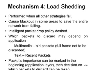
269. Announcements
• Midterm: November 28, Monday, 11:40 – 13:30
– Places:
FENS G032 if (lastName[0] >= 'A' && lastName[0] <=
'D')
FASS G022 if (lastName[0] >= 'E' && lastName[0] <=
'Ö')
FASS G049 if (lastName[0] >= 'P' && lastName[0] <=
'Z')
• Exam will be closed book, closed notes
– calculators are allowed
– you are responsible all topics I covered in the class even if some of
them are not in the book (I sometimes used other books) and not in
the ppt files (I sometimes used board and showed applications on
the computer)
269

270. Flow Control
• In Data Link Layer, we deal with issues
related to point to point links
– Flow control is one of these issues
• Flow control is needed since the sending
entity should not overwhelm the receiving
entity
– Recipient needs some time to process
incoming packets
– If sender sends faster than recipient
270

271. Performance Metrics and
Delays (Section 5.3)
• Transmission time (delay)
– Time taken to emit all bits into medium
• Propagation time (delay)
– Time for a bit to traverse the link
• Processing time (delay)
– time spent at the recipient or intermediate
node for processing
• Queuing time (delay)
– waiting time at the queue to be sent out
271

272. Model of Frame Transmission
transmission
time
propagation
time
272

273. Stop and Wait Flow Control
• Source transmits frame
• Destination receives frame and replies
with acknowledgement (ACK)
• Source waits for ACK before sending next
frame
• Destination can stop flow by not sending
ACK
• Works well for large frames
• Inefficient for smaller frames 273

274. Stop and Wait Flow Control
• However, generally large block of data split
into small frames
– Called “Fragmentation”
– Advantages are
• Limited buffer size at receiver
• Errors detected sooner (when whole frame received)
– On error, retransmission of smaller frames is needed
• Prevents one station occupying medium for long
periods
• Channel Utilization is higher when
– the transmission time is longer than the
propagation time
– frame length is larger than the bit length of the
274

275. Stop and Wait Link Utilization -
Details are on the board
propagation time = D, transmission time = T
t0 + T
t0 + T
t0 + D
t0 + D
t0 +T+D t0 +T+D
t0 +T+2D t0 +T+2D
D> T D< T
275

276. Sliding Window Flow Control
• The problem of “Stop and Wait” is not able to send
multiple packets
• Sliding Window Protocol allows multiple frames to be in
transit
• Receiver has buffer of W (called window size) frames
• Transmitter can send up to W frames without ACK
• Each frame is numbered
– Sequence number bounded by size of the sequence number
field (k bits)
– thus frames are numbered modulo 2k (0 … 2k-1)
• ACK includes number of next frame expected
276

277. Sliding Window Flow Control
(W = 7)
277

278. Example of a Sliding Window
Protocol (W = 7)
278

279. Sliding Window Enhancements
in Implementation
• Receiver can acknowledge frames without
permitting further transmission (Receive
Not Ready)
– Must send a normal acknowledgement to
resume
• If the link is duplex, use piggybacking
– Send data and ack together in one frame
• frame has both data and ack fields
– If no data to send, use acknowledgement
frame
– If data but no acknowledgement to send,
279

280. Sliding Windows Performance -
1
• two cases: W >= 2a+1 and W < 2a+1, where a=D/T
• details are on board

T
2T
D
D+T
2D+T
( W.T ≥ 2D+T ) 280

281. Sliding Windows Performance -
2
T
W.T
D
D+T
2D+T
( W.T < 2D+T )
281

282. Error Detection and Control
• So far we have seen flow control
mechanisms where frames are transmitted
without errors
– in real life any transmission facility may
introduce errors
• So we have to
– detect errors
– if possible, correct errors (not in the scope of
CS 408)
– adopt flow control algorithms such that 282

283. Types of Errors
• Single bit errors
– isolated errors
– affects (flips) one bit, nearby bits are not
altered
– not so common in real life
• Burst errors
– a sequence of bits are affected
– most common case
– a burst error of length B is a contiguous
sequence of B bits in which the first and the
last and some intermediate bits are 283

284. Error Detection
• Additional bits added by transmitter as
error detection code
– receiver checks this code
• Parity
– single bit added to the end of the data
– Value of parity bit is such that data and parity
have even (even parity) or odd (odd parity)
number of ones
– Even number of bit errors goes undetected 284

285. Error Detection Process using
Cyclic Redundancy Check
-
F= F’=
285

286. Cyclic Redundancy Check
(CRC)
• For a data block of k bits, transmitter
generates n-k bit frame check sequence
(FCS) and appends it to the end of the data
bits
• Transmits n bits, which is exactly divisible
by some number (generator)
– the length of the generator is n-k+1 and first
and last bits are 1
• Receiver divides the received frame by
generator
– If no remainder, assume no error 286

287. Cyclic Redundancy Check
(CRC)
• Standard CRCs (generators are standard)
– checks all single, double and odd number of
errors
– checks all burst errors with length less than or
equal to the length of FCS (n-k)
– checks most of the burst errors of longer
length
• for bursts of length n-k+1 (length of generator),
probability of an undetected error is 1/2n-k-1
• for longer bursts, probability of an undetected error
is 1/2n-k
287

288. Error Control
• Actions to be taken against
– Lost frames
– Damaged frames
• Automatic repeat request (ARQ)
mechanism components
– Error detection
– Positive acknowledgment
– Retransmission after timeout
– Negative acknowledgement and
retransmission 288

289. Automatic Repeat Request
(ARQ)
• Stop-and-wait ARQ
• Go-back-N ARQ
• Selective-reject (selective retransmission)
ARQ
289

290. Stop and Wait ARQ
• Source transmits single frame
• Wait for ACK
• If received frame is damaged, discard it
– If transmitter receives no ACK within timeout,
retransmits
• If ACK damaged,transmitter will not
recognize it
– Transmitter will retransmit after timeout
– Receiver gets two copies of frame, but
disregards one of them
– Use ACK0 and ACK1
290

291. Stop-and-Wait ARQ –
Example
291

292. Stop and Wait - Pros and Cons
• Simple
• Inefficient
292

293. Go-Back-N ARQ
• Based on sliding window
• If no error, ACK as usual with next frame
expected
– ACKi means “I am ready to receive frame i”
and “I received all frames between i and my
previous ack”
• Sender uses window to control the
number of unacknowledged frames
• If error, reply with rejection (negative ack)
– Discard that frame and all future frames until
the frame in error is received correctly
– Transmitter must go back and retransmit that
293

294. Go-Back-N ARQ -
Damaged Frame
• Receiver detects error in frame i
• Receiver sends “reject i”
• Transmitter gets “reject i”
• Transmitter retransmits frame i and all
subsequent frames
294

295. Go-Back-N ARQ - Lost Frame
(1)
• Frame i lost
• Transmitter sends frame i+1
• Receiver gets frame i+1 out of sequence
• Receiver sends “reject i”
• Transmitter goes back to frame i and
retransmits it and all subsequent frames
295

296. Go-Back-N ARQ- Lost Frame
(2)
• Frame i lost and no additional frame sent
• Receiver gets nothing and returns neither
acknowledgment nor rejection
– This is kind of a deadlock situation that needs to be resolved
• Transmitter times out and sends
acknowledgment frame with P bit set to 1
(this is actually a command for ack request)
– Receiver interprets this as an ack request
command which it acknowledges with the
number of the next frame it expects (i )
• Transmitter then retransmits frame i
296

297. Go-Back-N ARQ-
Damaged/Lost
Acknowledgment
• Receiver gets frame i and sends
acknowledgment (i+1) which is lost
• Acknowledgments are cumulative, so next
acknowledgement (i+n) may arrive before
transmitter times out on frame i
==> NO PROBLEM
• If transmitter times out, it sends
acknowledgment request with P bit set, as
before
297

298. Go-Back-N ARQ- Damaged
Rejection
• As in lost frame (2)
– sender asks the receiver the last frame
received and continue by retransmitting next
frame
298

299. Go-Back-N ARQ -
Example
299

300. Selective Reject
• Also called selective retransmission
• Only rejected frames are retransmitted
• Subsequent frames are accepted by the
receiver and buffered
• Minimizes retransmissions
• Receiver must maintain large enough
buffer
• Complex implementation
300

301. Selective Reject -
Diagram
301

302. Issues
• RR with P=1 is from HDLC standard
– pure protocol just have retransmissions after
timeout
• as explained in Tanenbaum
302

303. Issues – Window Size
• Given n-bit sequence numbers, what is
Max window size?
– go-back-n ARQ  2n-1
• Why?
• what about receiver’s window size?
– It is 1, why?
– selective-reject(repeat)  2n-1
• Why?
• See the reasons on the board
303

304. Issues – Buffer Size
• Go-back-n ARQ
– sender needs to keep a buffer equal to
window size
• for possible retransmissions
– receiver does not need any buffer (for
flow/error control)
• why?
• Selective reject
– sender needs to keep a buffer of window size
for retransmissions
– receiver keeps a buffer equal to window size
304

305. Issues - Performance
• Notes on board
• Appendix at the end of Chapter 14
– selective reject ARQ is not in the book
305

306. High Level Data Link Control
• HDLC
• ISO Standard
• Basis for some other DLL protocols
306

307. HDLC Station Types
• Primary station
– Controls operation of link
– Frames issued are called commands
• Secondary station
– Under control of primary station
– Frames issued called responses
• Combined station
– May issue commands and responses
307

308. HDLC Link Configurations
• Unbalanced
– One primary and one or more secondary
stations
– Supports full duplex and half duplex
• Balanced
– Two combined stations
– Supports full duplex and half duplex
308

309. HDLC Transfer Modes (1)
• Normal Response Mode (NRM)
– Unbalanced configuration
– Primary initiates transfer to secondary
– Secondary may only transmit data in
response to command from primary
– Terminal-host communication
• Host computer as primary
• Terminals as secondary
– not so common nowadays
309

310. HDLC Transfer Modes (2)
• Asynchronous Balanced Mode (ABM)
– Balanced configuration
– Either station may initiate transmission
without receiving permission
– Most widely used
310

311. Frame Structure
• All transmissions in frames
• Single frame format for all data and
control exchanges
311

312. Frame Structure Diagram
312

313. Flag Fields
• Delimit frame at both ends
• 01111110
• Receiver hunts for flag sequence to
synchronize
• Bit stuffing used to avoid confusion with
data containing 01111110
– 0 inserted after every sequence of five 1s
– If receiver detects five 1s after a 0 it checks
next bit
• If 0, it is deleted
313

314. Bit Stuffing Example
314

315. Address Field
• Identifies secondary station that sent or
will receive frame
• Usually 8 bits long (but 7 bits are effective)
• May be extended to multiples of 7 bits with
prior agreement
– leftmost bit of each octet indicates that it is
the last octet (1) or not (0)
315

316. Frame Types
• Information frame- data to be transmitted to
user
– Acknowledgment is piggybacked on information
frames (only for positive acknowledgment)
• Supervisory frame – ARQ messages
(RR/RNR/REJ/SREJ) when piggyback not
used (actually only RR can be piggybacked;
for the other, we need Supervisory frames)
• Unnumbered frame – supplementary link
control functions. For examples,
– setting the modes 316

317. Control Field Diagram
317

318. Poll/Final Bit
• Use of this bit depends on context. A
typical use is below.
• Command frame
– P bit set to 1 to solicit (poll) supervisory frame
from peer
• Response frame
– F bit set to 1 to indicate response to soliciting
command
318

319. Information Field
• Only in information and some unnumbered
frames
• Must contain integral number of octets
• Variable length
319

320. Frame Check Sequence Field
• FCS
• Error detection
• 16 bit CRC
• Optional 32 bit CRC
320

321. HDLC Operation
• Exchange of information, supervisory and
unnumbered frames
• Three phases
– Initialization
– Data transfer
– Disconnect
321

322. Initialization
• Issue one of six set-mode commands
– Signals other side that initialization is
requested
– Specifies mode (NRM, ABM, ARM)
– Specifies 3- or 7-bit sequence numbers
• If request accepted, HDLC module on
other side transmits "unnumbered
acknowledged" (UA) frame
• If request rejected, "disconnected mode"
(DM) sent 322

323. Data Transfer
• Both sides may begin to send user data in I-frames (Information
Frame)
– N(S): sequence number of outgoing I-frames
• modulo 8 or 128, (3- or 7-bit)
– N(R) acknowledgment for I-frames received
• seq. number of I-frame expected next
• S-frames are also used for flow and error control
– Receive ready (RR) frame acknowledges last I-frame received
• Indicating next I-frame expected
• Used when there is no reverse data
– Receive not ready (RNR) acknowledges, but also asks peer to suspend
transmission of I-frames
• When ready, send RR to restart
– REJ initiates go-back-N ARQ
• Indicates last I-frame received has been rejected
• Retransmission is requested beginning with N(R)
– Selective reject (SREJ) requests retransmission of single frame 323

324. Disconnect
• Send disconnect (DISC) frame
• Remote entity must accept by replying
with UA
– Informs layer 3 user about the termination of
connection
• These frames are unnumbered frames
324

325. Examples of Operation (1)
325

326. Examples of Operation (2)
326

327. Other DLC Protocols
(LAPB,LAPD)
• Link Access Procedure, Balanced (LAPB)
– Part of X.25 (ITU-T)
– Subset of HDLC - ABM (Async. Balanced
Mode)
– Point to point link between user and packet
switching network node
– HDLC frame format
• Link Access Procedure, D-Channel
(LAPD)
– Part of ISDN (ITU-T)
– ABM
– Always 7-bit sequence numbers (no 3-bit)
327

328. Other DLC Protocols (LLC)
• Logical Link Control (LLC)
– IEEE 802
– For LANs (Local Area Networks)
– Link control split between medium access control layer (MAC) and
LLC (on top of MAC)
– Different frame format
• Two addresses needed (sender and receiver) – actually at MAC layer
• Sender and receiver SAP addresses
• Control field is same as HDLC (16-bit version for I and S frames; 8-bit
for U frames)
– No primary and secondary - all stations are peers
– Error detection at MAC layer
• 32 bit CRC
328

329. Other DLC Protocols (LLC)
• LLC Services
– 3 alternatives
– Connection Mode Services
• Similar to HDLC ABM
– Unacknowledged connectionless services
• no connection setup
• No flow-control, no error control, no acks (thus not
reliable)
• good to be used with TCP/IP. Why?
– Acknowledged Connectionless Service
• No connection setup 329

330. VLANs
330

331. Topics
• The role of VLANs in a network
• Trunking VLANs
• Configure VLANs on switches
• Troubleshoot common VLAN problems
331

332. Semester 3
LAN Design
Basic Switch
Concepts
VLANs
VTP
STP
Inter-VLAN
routing
Wireless
332

333. Some requirements of LANs
• Need to split up broadcast domains to
make good use of bandwidth
• People in the same department may need
to be grouped together for access to
servers
• Security: restrict access by certain users
to some areas of the LAN
• Provide a way for different areas of the
LAN to communicate with each other
333

334. Solution using routers
• Divide the LAN into
subnets
• Use routers to link
the subnets
334

335. Solution using routers
BUT
• Routers are expensive
• Routers are slower than switches
• Subnets are restricted to limited physical
areas
• Subnets are inflexible
335

336. Solution using VLANs
• VLAN membership can
be by function and not
by location
• VLANs managed by
switches
• Router needed for
communication
between VLANs
336

337. VLANs
• All hosts in a VLAN have addresses in the
same subnet. A VLAN is a subnet.
• Broadcasts are kept within the VLAN. A
VLAN is a broadcast domain.
• The switch has a separate MAC address
table for each VLAN. Traffic for each VLAN
is kept separate from other VLANs.
• Layer 2 switches cannot route between
VLANs. 337

338. VLAN numbers
• VLAN 1: default Ethernet LAN, all ports start
in this VLAN.
• VLANs 1002 – 1005 automatically created
for Token Ring and FDDI
• Numbers 2 to 1001 can be used for new
VLANs
• Up to 255 VLANs on Catalyst 2960 switch
• Extended range 1006 – 4094 possible but
fewer features 338

339. VLAN information
• VLAN information is stored in the VLAN
database.
• vlan.dat in the flash memory of the switch.
339

340. Port based
• Each switch port intended for an end
device is configured to belong to a VLAN.
• Any device connecting to that port belongs
to the port’s VLAN.
• There are other ways of assigning VLANs
but this is now the normal way.
• Ports that link switches can be configured
to carry traffic for all VLANs (trunking)
340

341. Types of VLAN
• Data or user VLAN
• Voice VLAN
• Management VLAN
• Native VLAN
• Default VLAN
341

342. Data VLAN
• Carry files, e-mails, shared application
traffic, most user traffic.
• Separate VLAN for each group of users.
342

343. Voice VLAN
• Use with IP phone.
• Phone acts as a switch too.
• Voice traffic is tagged, given priority.
• Data not tagged, no priority.
343

344. Management VLAN
• Has the switch IP address.
• Used for telnet/SSH or web access for
management purposes.
• Better not to use VLAN 1 for security
reasons.
344

345. Native VLAN
• For backward compatibility with older
systems.
• Relevant to trunk ports.
• Trunk ports carry traffic from multiple
VLANs.
• VLAN is identified by a “tag” in the frame.
• Native VLAN does not have a tag.
345

346. Default VLAN
• VLAN 1 on Cisco switches.
• Carries CDP and STP (spanning tree
protocol) traffic.
• Initially all ports are in this VLAN.
• Do not use it for data, voice or
management traffic for security reasons.
346

347. Static VLAN
• The normal type. Port configured to be on
a VLAN. Connected device is on this
VLAN.
• VLAN can be created using CLI command,
given number and name.
• VLAN can be learned from another switch.
• If a port is put on a VLAN and the VLAN
does not exist, then the VLAN is created.
347

348. Static VLAN (Port-centric)
• If VLAN 20 did not exist before – then it
does now.
348

349. Voice VLAN
• Configured for voice VLAN and data
VLAN.
349

350. Dynamic VLAN
• Not widely used.
• Use a VLAN Membership Policy Server
(VMPS).
• Assign a device to a VLAN based on its
MAC address.
• Connect device, server assigns VLAN.
• Useful if you want to move devices
around.
350

351. Traffic between VLANs
• Layer 2 switch keeps VLANs separate.
• Router can route between VLANs. It
needs to provide a default gateway for
each VLAN as VLANs are separate
subnets.
• Layer 3 switch has a switch virtual
interface (SVI) configured for each VLAN.
These act like router interfaces to route
between VLANs.
351

352. Trunking
• Both switches have the same 5 VLANs.
• Do you have a link for each VLAN?
• More efficient for them to share a link.
352

353. Trunking
• Traffic for all the VLANs travels between the
switches on a shared trunk or backbone

354. Tag to identify VLAN
• Tag is added to the frame when it goes on to the
trunk
• Tag is removed when it leaves the trunk

355. Frame tagging IEEE 802.1Q
Dest Add Source Add Type/Len Data FCS
Dest Add Source Add Type/Len Data FCS
Tag
Normal
frame
Add 4-byte tag,
recalculate FCS
Tag protocol
ID 0x8100
Priority CFI for token
ring
VLAN ID
1 - 4096
355

356. Native VLAN
• Untagged frames received on a trunk port
are forwarded on to the native VLAN.
• Frame received from the native VLAN
should be untagged.
• Switch will drop tagged frames received
from the native VLAN. This can happen if
non-Cisco devices are connected.
356

357. Configure trunk port
• Make a port into a trunk port and tell it
which VLAN is native.
• SW1(config)#int fa0/1
• SW1(config-if)switchport mode trunk
• SW1(config-if)switchport trunk native
vlan 99
• By default native VLAN is 1.
357

358. Dynamic trunking protocol
Mode
trunk
Dynamic
auto/des
Mode
access
access
trunk
access
Dynamic
auto
Dynamic
auto
trunk Dynamic
desirable
Dynamic
desirable
Dynamic
auto/des
Dynamic
desirable
Dynamic
auto
trunk
358

359. Create a VLAN
• SW1(config)#vlan 20
• SW1(config-vlan)#name Finance
• SW1(config-vlan)#end
• VLAN will be saved in VLAN database
rather than running config.
• If you do not give it a name then it will be
called vlan0020.
359

360. Assign port to VLAN
• SW1(config)#int fa 0/14
• SW1(config-if)#switchport mode access
• SW1(config-if)#switchport access vlan
20
• SW1(config-if)#end
360

361. show vlan brief
• List of VLANs with ports
361

362. Show commands
• show vlan brief (list of VLANs and ports)
• show vlan summary
• show interfaces vlan (up/down, traffic etc)
• Show interfaces fa0/14 switchport (access
mode, trunking)
362

363. Remove port from VLAN
• SW1(config)#int fa 0/14
• SW1(config-if)#no switchport access
vlan
• SW1(config-if)#end
• The port goes back to VLAN 1.
• If you assign a port to a new VLAN, it is
automatically removed from its existing
VLAN.
363

364. Delete a VLAN
• SW1(config)#no vlan 20
• SW1(config)#end
• VLAN 20 is deleted.
• Any ports still on VLAN 20 will be inactive
– not on any VLAN. They need to be
reassigned.
364

365. Delete VLAN database
• Erasing the startup configuration does not
get rid of VLANs because they are saved
in a separate file.
• SW1#delete flash:vlan.dat
• Switch goes back to the default with all
ports in VLAN 1.
• You cannot delete VLAN 1.
365

366. The Network Layer
Design Issues & Routing Algorithms
UNIT-3
366

367. Network Layer Design Isues
• Store-and-Forward Packet Switching
• Services Provided to the Transport Layer
• Implementation of Connectionless Service
• Implementation of Connection-Oriented Service
• Comparison of Virtual-Circuit and Datagram Subnets
367

368. Store-and-Forward Packet
Switching
The environment of the network layer
protocols.
fig 5-1
368

369. Services Provided to the
Transport Layer
1.The services should be independent of the
router technology
2.The transport layer should be shielded
from the number, type and topology of the
routers present
3.The network addresses made available to
the transport layer should use a uniform
numbering plan, even across LANs and
WANs 369

370. Implementation of Connectionless
Service
Routing within a diagram subnet.
370

371. Implementation of Connection-
Oriented Service
Routing within a virtual-circuit subnet. 371

372. Comparison of Virtual-Circuit and
Datagram Subnets
5-4
372

373. Routing Algorithms
• The Optimality Principle
• Shortest Path Routing
• Flooding
• Distance Vector Routing
• Link State Routing
• Hierarchical Routing
• Broadcast Routing
• Multicast Routing
• Routing for Mobile Hosts
• Routing in Ad Hoc Networks 373

374. Desirable Properties (Elaborate)
Correctness
Simplicity
Robustness – System will be in place for
years with small failures
Stability – Fast convergence
Fairness,
Efficiency.
374

375. Routing Algorithms (2)
Conflict between fairness and optimality.
Minimizing the mean packet delay is an obvious
A – A’, B – B’, C – C’, can fill the channel, then X-X’ doesn’t get a chance
375

376. Elaborate
• Adaptive/Non-adaptive routing
376

377. The Optimality Principle
(a) A subnet. (b) A sink tree for router
B.
Optimality Principle – If router J is on the optimal path from router I to router K
then the optimal path from J to K also falls along the same route.
377

378. Shortest Path Routing
The first 5 steps used in computing the
shortest path from A to D.
The arrows indicate the working node.
378

379. Dijkstra
Dijkstra's algorithm to compute the shortest path
5-8 top
379

380. Dijkstra
Dijkstra's algorithm to compute the shortest path
5-8
bottom
380

381. Flooding
Robust but costly.
TTL and keep track…
•Used in military application
•Wireless Networks
•Distributed Database
•Metrics against which other routing
algorithms are compared.
381

382. Distance Vector Routing
(a) A subnet. (b) Input from A, I, H, K, and the
new 382

383. Distance Vector Routing (2)
The count-to-infinity problem. 383

384. Hierarchical Routing
Hierarchical routing.
Problems – optimal paths are sacrificed
384

385. Hierarchical Routing (2)
• How many levels of hierarchy?
• 720 routers.
• 720 routers in 24 regions.
• Three levels of hierarchy – 8 clusters each
containing 9 regions of 10 clusters.
385

386. Link State Routing
Each router must do the following:
1.Discover its neighbors, learn their network address.
2.Measure the delay or cost to each of its neighbors.
3.Construct a packet telling all it has just learned.
4.Send this packet to all other routers.
5.Compute the shortest path to every other router.
386

387. Learning about the Neighbors
(a) Nine routers and a LAN. (b) A graph
model of (a). All routers 387

388. Setting Link Cost
• Bandwidth
• Delay – measured by sending special ECHO
• Geographically spread out links
388

389. Measuring Line Cost
• A subnet in which the East and West parts are
connected by 2 lines.
• Including queuing delay may lead to a lot of
389

390. Building Link State Packets
(a) A subnet. (b) The link state packets
for this subnet. 390

391. Few Problems
Algorithm – Sequence number less means
obsolete
• If sequence numbers wrap around,
confusion will reign
• Router crashes, sequence number is lost
• Sequence number gets corrupted
•Aging and then dropping the packet. 391

392. Distributing the Link State
Packets
• The packet buffer for router B in the previous
slide (Fig. 5-13).
• E has arrived twice. 392

393. OSPF (Open Shortest Path First)
IS-IS (intermediate System-
Intermediate System)
• Refreshed every 60 seconds.
• Hardware problem, router getting corrupt, etc.
393

394. Broadcast Routing
Multidimensional Routing
•Each packet contains a list of destinations.
•On arrival of a packet, router checks the set of destinations, and sends
copies of packet along outgoing links to those destinations.
Flooding
•Flood with a sequence number per source.
Spanning Tree
•Build spanning tree (such as, a sink tree).
•Forward packet along all links of spanning tree except the one from
which packet is received.
Reverse Path Forwarding 394

395. Broadcast – Reverse Path
Forwarding
• Broadcast.
• Check if the packet has arrived following the correct hop
or not.
• If correct hop, then rebroadcast.
Reverse path forwarding.
(a) A subnet. (b) a Sink tree. 395

396. Multicast Routing
(a) A network. (b) A spanning tree for the leftmost router.
(c) A multicast tree for group 1. (d) A multicast tree for group 2.
Typically done in Multi-state routing
396

397. Anycast Routing
• Reaching any one of the servers in the group
• DNS server
397

398. Routing for Mobile Hosts
A WAN to which LANs, MANs, and wireless
cells are attached.
398

399. Routing for Mobile Hosts (2)
Packet routing for mobile users.
399

400. Routing in Ad Hoc Networks
Possibilities when the routers are mobile:
1.Military vehicles on battlefield.
– No infrastructure.
2.A fleet of ships at sea.
– All moving all the time
3.Emergency works at earthquake .
– The infrastructure destroyed.
4.A gathering of people with notebook computers.
– In an area lacking 802.11.
400

401. Ad Hoc Networks: Route
Discovery
(a) Range of A's broadcast.
(b) After B and D have received A's
broadcast.
(c) After C, F, and G have received A's
broadcast. 401

402. Route Discovery (2)
Format of a ROUTE REQUEST packet.
402

403. Route Discovery (3)
• The (Source Address, Request ID) pair is looked up in a
local history table
• Receiver looks up the destination in its route table. If a
fresh route is known, then a ROUTE REPLY is sent.
• Destination sequence number is higher than the
Destination sequence in the Route Discovery Packet
• Increments Hop count and rebroadcasts ROUTE REPLY
• Stores the data in a new entry in its reverse route table.
403

404. Route Discovery (4)
Format of a ROUTE REPLY packet.
404

405. Route Discovery (5)
IN response
•Source addr., destination addr. and Hop Count copied but
Dest. Seq. number taken from its counter.
•Hopcount is set to 0, Lifetime field controls how long the
route is valid.
At each intermediate node:
1.No route to I is known,
2.Sequence number of I in the ROUTE REPLY packet is
greater than the value in the routing table
3.The sequence numbers are equal but the new route is
shorter
4.Hop Count incremented
5.In large network, discovery increases with Time to Live
incrementally being increased from 1, 2, 3, …
405

406. Ad Hoc Networks: Route
Maintenance
Active Neighbours that have fed in those
destinations to A in last t seconds
(a) D's routing table before G goes down.
(b) The graph after G has gone down. 406

407. Routing for Mobile Hosts
A WAN to which LANs, MANs, and wireless
cells are attached.
407

408. Routing for Mobile Hosts (2)
Packet routing for mobile users.
408

409. Routing in Ad Hoc Networks
Possibilities when the routers are mobile:
1.Military vehicles on battlefield.
– No infrastructure.
2.A fleet of ships at sea.
– All moving all the time
3.Emergency works at earthquake .
– The infrastructure destroyed.
4.A gathering of people with notebook computers.
– In an area lacking 802.11.
409

410. AODV
Adhoc On-demand Distance
Vector
410

411. Ad Hoc Networks: Route
Discovery
(a) Range of A's broadcast. (Maintains a
distance vector routing table)
(b) After B and D have received A's
broadcast.
(c) After C, F, and G have received A's 411

412. Route Discovery (2)
Format of a ROUTE REQUEST packet.
412

413. Route Discovery (3)
• The (Source Address, Request ID) pair is looked up in a
local history table
• Receiver looks up the destination in its route table. If a
fresh route is known, then a ROUTE REPLY is sent.
• Destination sequence number is higher than the
Destination sequence in the Route Discovery Packet
• Increments Hop count and rebroadcasts ROUTE REPLY
• Stores the data in a new entry in its reverse route table.
413

414. Route Discovery (4)
Format of a ROUTE REPLY packet.
414

415. Route Discovery (5)
IN response
•Source addr., destination addr. and Hop Count copied but
Dest. Seq. number taken from its counter.
•Hopcount is set to 0, Lifetime field controls how long the
route is valid.
At each intermediate node:
1.No route to I is known,
2.Sequence number of I in the ROUTE REPLY packet is
greater than the value in the routing table
3.The sequence numbers are equal but the new route is
shorter
4.Hop Count incremented
5.In large network, discovery increases with Time to Live
incrementally being increased from 1, 2, 3, …
415

416. Ad Hoc Networks: Route
Maintenance
Active Neighbours that have fed in those
destinations to A in last t seconds
(a) D's routing table before G goes down.
(b) The graph after G has gone down. 416

417. Node Lookup in Peer-to-Peer
Networks
P2P: Large connection of computers, without central control
where typically each node has some information of interest.
• No central control for routing
• No central data repository
Two basic questions:
1. How to make data at each node available?
2. How to find required information?
The questions are interrelated, but will be looked at separately.
417

418. Assumption
• Each record (data to be shared) can be
identified by a ASCII string such as the
filename.
Over the past 3-4 years, there has been several
proposals for P2P architectures we shall look at
Chord.
418

419. Basics of Chord
• Uses a hash function such as SHA-1.
• SHA-1 converts a variable length input into a highly
random 160 bit value
• Using SHA-1, Chord hashes:
node IP addresses node identifiers (160
bits)
names of records keys (160
bits) 419

420. Storing Records
(a) A set of 32 node identifiers arranged in a
circle. The shaded ones correspond to
actual machines. The arcs show the fingers
420

421. Storing records
• successor (k) is the first real node after k.
• To store data name, a node N creates a tuple (name, N's
IP address) and stores the tuple at
successor(hash(name)). The original data remain at N,
just the tuple is stored at successor(hash(name)).
• If hash(name) = 22, then the tuple is stored at node 27.
• To find information name, a node does key = hash(name),
then gets the record tuple from successor(key).
• Simple? Mostly, except for implementing successors(key)
efficiently. 421

422. Finding records
Each node needs to store the IP addresses of its successor.
Initially, the network start out with just a few nodes:
1. All nodes know each other.
2. They can easily arrange themselves into a the Chord ring.
3. successor(k) can be computed.
When a node tries to join:
1. It calculates its node ID say p.
2. Then asks any node already in the ring to find successor(p).
3. Asks successor(p) for successor(p)'s predecessor and
inserts itself between them.
Any node in the ring can find successor(k) by propagating the
query around the ring starting with its successor. 422

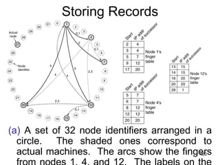
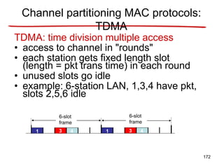
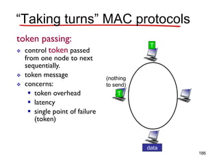
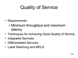
423. Finger table
• Even if both successor and predecessor pointers are
used, a sequential search will take time on average
O(n/2) [n is the number of nodes].
• Chord reduces this search time using a finger table at
each node.
• The finger table contains up to m entries where each
entry i consists of IP address of successor(start[i])
• Start[i] = k + 2^i (modulo 2^m)
• To find a record for key k, a node can directly jump to
the closest predecessor of k.
• Average time can be reduced to O(log n).
423

424. Looking up key 16 at node 1
1. Nearest pred. 9 so query sent to 12
2. At 12 nearest pred. of 16 is 14 so query sent
to 15
3. 15 knows that 16 is between itself and its
successor so 15 send back 20's IP address
to 1.
424

425. Maintaining finger table
• Maintaining the finger table does not come for
free.
• Every time a new node is added a few
successors and predecessor entries will
change.
425

426. The Network Layer
Congestion Control Algorithms &
Quality-of-Service
426

427. Congestion Control Algorithms
• Approaches to Congestion Control
• Traffic-Aware Routing
• Admission Control
• Traffic Throttling
• Load Shedding
427

428. Congestion
When too much traffic is offered, congestion
sets in and performance degrades sharply.
428

429. General Principles of Congestion
Control
1.Monitor the system
–detect when and where congestion occurs.
2.Pass information to where action can be
taken.
3.Adjust system operation to correct the
problem.
4.Difference between Congestion control and
flow control – Elaborate 429

430. Approaches to Congestion
Control
Two solutions possible:
1)Increase resources
2)Decrease load
430

431. Traffic-Aware Routing
A network in which the East and West parts
are connected by two links. 431

432. Admission Control
(a)A congested network. (b) The portion of
the network that is not congested. A virtual
circuit from A to B is also shown.
Problem is in virtual circuits – there may be
432

433. Traffic Throttling:Congestion
Detection
• Routers must determine when congestion is approaching,
ideally before it has arrived.
• Each router can continuously monitor the resources it is
using.
• 3 possibilities:
1. utilization of the output links
2. buffering of queued packets inside the router (most
useful)
3. no. of packets that are lost due to insufficient buffering
EWMA (Exponentially Weighted Moving Average)
• dnew = αdold + (1 − α)s,
where, the constant α determines how fast the router
forgets recent history. 433

434. Traffic Throttling: Feedback
• Routers must deliver timely feedback to the senders that
are causing the congestion.
• The router must identify the appropriate senders.
• It must then warn them carefully, without sending many
more packets into the already congested network.
• Many feedback mechanisms:
Mechanism 1: Explicit Congestion Notification (ECN)
434

435. Mechanisms 2 & 3:
Direct Choke Packets,
Hop-by-Hop
Backpressure
M-2: A choke packet
that affects only the
source.
M-3: A choke packet
that affects each
hop it passes
through. 435

436. Mechanism 4: Load Shedding
• Performed when all other strategies fail.
• Cause blackout in some areas to save the entire
network from failing.
• Intelligent packet drop policy desired.
• Which packets to discard may depend on
application
Multimedia – old packets (full frame not to be
discarded)
Text – Recent Packets
• Packet’s importance can be marked in the
beginning (application layer), then decision on 436

437. Mechanism 5: Random Early
Detection
• Discard packets before all the buffer space is
really exhausted.
• To determine when to start discarding, routers
maintain a running average of their queue
lengths.
• When average queue length exceeds a
threshold, the link is said to be congested –
small fraction of packets dropped at random.
• The affected sender will notice the loss when
there is no acknowledgement – transport
protocol slowed down. 437

438. Quality of Service
• Requirements
• Minimum throughput and maximum
latency
• Techniques for Achieving Good Quality of Service
• Integrated Services
• Differentiated Services
• Label Switching and MPLS
438

439. Requirements
How stringent the quality-of-service
requirements are.
5-30
439

440. Categories of QoS and Examples
1.Constant bit rate
• Telephony
2.Real-time variable bit rate
• Compressed videoconferencing
3.Non-real-time variable bit rate
• Watching a movie on demand
4.Available bit rate
• File transfer 440

441. Jitter Control
(a) High jitter. (b) Low
Schedule Delay according to Deadline Miss
441

442. Buffering
Smoothing the output stream by buffering
packets.
442

443. Traffic Shaping
• Traffic in data networks is bursty – typically
arrives at non-uniform rates as the traffic rate
varies.
• Traffic shaping is a technique for regulating
the average rate and burstiness of a flow of
data that enters the network.
• When a flow is set up, the user and the
network agree on a certain traffic pattern
(shape).
• Sometimes this agreement is called an SLA
(Service Level Agreement).
443

444. The Leaky Bucket Algorithm
(a) A leaky bucket with water. (b) a leaky
bucket with packets.
444

445. The Token Bucket Algorithm
(a) Before. (b) After.
5-34
445

446. Token Bucket Algorithm (2)
• Burst length – S sec.
• Maximum output rate – M bytes/sec
• Token bucket capacity – B bytes
• Token arrival rate – R bytes/sec
• An output burst contains a maximum of (B + RS)
bytes.
• The number of bytes in a maximum speed burst of
length S seconds is MS.
• Hence, we have: B + RS = MS
• This equation can be solved to get S = B /(M − R)
446

447. Traffic Shaping (2)
(a) Traffic from a host. Output shaped by a
token bucket of rate 200 Mbps and capacity (b)
447

448. Traffic Shaping (3)
Token bucket level for shaping with rate 200
Mbps and capacity (d) 16000 KB, (e) 9600448

449. Packet Scheduling
Kinds of resources that can potentially be
reserved for different flows:
1. Bandwidth.
2. Buffer space.
3. CPU cycles.
449

450. Packet Scheduling (2)
Round-robin Fair Queuing
450

451. Packet Scheduling (3)
(a)Weighted Fair Queueing.
(b)Finishing times for the packets.
451

452. Admission Control (1)
An example flow specification
452

453. • T = 1/mu X 1/(1-lambda/mu) -- lambda
= 0.95Mpackets/sec
• mu = 1Mb packets/sec
453

454. Admission Control (2)
Bandwidth and delay guarantees with token
buckets and WFQ.
454

455. Integrated Services:
RSVP—The Resource reSerVation Protocol
(a) A network. (b) The multicast spanning tree
455

456. Hosts 1 and 2 are multicast sender
3,4, 5 are multicast receiver
Host 3 reserves for Host 1 and the Host 2
Host 5 reserves Host 1 (so the common path is
utilized). However depending on need (Host 5
may be a bigger TV) – provision is made for the
greediest part 456

457. RSVP (2)
(a) Host 3 requests a channel to host 1. (b) Host
3 then requests a second channel, to host 2.
457

458. Differentiated Services:
Expedited Forwarding
Expedited packets experience a traffic-free
network 458

459. Class-Based Service
Per Hop Behaviors
Traffic within a class are given preferential
treatment
Expedited Forwarding
Packets marked – Regular or Expedited
Assured Forwarding
Gold, Silver, Bronze, common 459

460. Differentiated Services:
Assured Forwarding
A possible implementation of assured
forwarding, weighted fair scheduling, RED
460

461. The Leaky
Bucket
Algorithm
(a) Input to a leaky
bucket. (b) Output from a
leaky bucket. Output
from a token bucket with
capacities of (c) 250 KB,
(d) 500 KB, (e) 750 KB,
(f) Output from a 500KB
token bucket feeding a
10-MB/sec leaky bucket. 461

462. 462
Network Layer
Routing

463. 463
Network Layer
• Concerned with getting packets from source to
destination.
• The network layer must know the topology of the
subnet and choose appropriate paths through it.
• When source and destination are in different
networks, the network layer (IP) must deal with
these differences.
* Key issue: what service does the network layer
provide to the transport layer (connection-
oriented or connectionless).

464. 464
Network Layer Design Goals
1.The services provided by the network layer
should be independent of the subnet topology.
2.The Transport Layer should be shielded from
the number, type and topology of the subnets
present.
3.The network addresses available to the
Transport Layer should use a uniform
numbering plan (even across LANs and WANs).

465. 465
Figure 7.2
Physical
layer
Data link
layer
Physical
layer
Data link
layer
End system
a
Network
layer
Physical
layer
Data link
layer
Physical
layer
Data link
layer
Transport
layer
Transport
layer
Messages
Messages
Segments
End system
b
Network
service
Network
service
Copyright ©2000 The McGraw Hill Companies Leon-Garcia & Widjaja: Communication Networks
Network
layer
Networ
k
layer
Network
layer

466. 466
Application
Transport
Internet
Network
Interface
Application
Transport
Internet
Internet
Network 1 Network 2
Machine A Machine B
Router/Gateway
Network
Interface
Network
Interface
Figure 8.3

467. 467
R
R
R
R
S
S
S
s
s
s
s
s
s
s
s
s
s
R
s
R
Backbone
To internet or
wide area
network
Organization
Servers
Gateway
Departmenta
l Server
Figure 7.6
Copyright ©2000 The McGraw Hill Companies
Leon-Garcia & Widjaja: Communication Networks
Metropolitan Area
Network (MAN)

468. 468
Interdomain level
Intradomain level
LAN level
Autonomous system
or domain
Border routers
Border routers
Figure 7.7
Internet service
provider
Copyright ©2000 The McGraw Hill Companies
Leon-Garcia & Widjaja: Communication Networks
Wide Area Network
(WAN)

469. 469
RA
RB
RC
Route
server
NAP
National service provider A
National service provider B
National service provider C
LAN
NAP
NAP
(a)
(b)
Figure 7.8
Copyright ©2000 The McGraw Hill Companies
Leon-Garcia & Widjaja: Communication Networks
National ISPs
Network Access
Point

470. 470
Packet 2
Packet 1
Packet 1
Packet 2
Packet 2
Figure 7.15
Datagram Packet Switching
Copyright ©2000 The McGraw Hill Companies Leon-Garcia & Widjaja: Communication Networks

471. 471
Destination
address
Output
port
1345 12
2458
7
0785
6
12
1566
Figure 7.16
Routing Table
in Datagram Network
Copyright ©2000 The McGraw Hill Companies
Leon-Garcia & Widjaja: Communication Networks

472. 472
Packet
Packet
Figure 7.17
Copyright ©2000 The McGraw Hill Companies Leon-Garcia & Widjaja: Communication Networks
Virtual Circuit Packet Switching

473. 473
Identifier Output
port
15 15
58
13
13
7
27
12
Next
identifier
44
23
16
34
Entry for packets
with identifier 15
Figure 7.21
Copyright ©2000 The McGraw Hill Companies
Leon-Garcia & Widjaja: Communication Networks
Routing Table
in Virtual Circuit Network

474. 474
Routing
Routing algorithm:: that part of the
Network Layer responsible for deciding
on which output line to transmit an
incoming packet.
Remember: For virtual circuit subnets the
routing decision is made ONLY at set up.
Algorithm properties:: correctness,
simplicity, robustness, stability, fairness,
optimality, and scalability.

475. 475
Routing Classification
Adaptive Routing
• based on current
measurements
of traffic and/or topology.
1. centralized
2. isolated
3. distributed
Non-Adaptive
Routing
• routing computed in
advance and off-line
1. flooding
2. static routing
using shortest
path algorithms

476. 476
Flooding
• Pure flooding :: every incoming packet
to a node is sent out on every outgoing
line.
– Obvious adjustment – do not send out on
arriving link (assuming full-duplex links).
– The routing algorithm can use a hop
counter (e.g., TTL) to dampen the
flooding.
– Selective flooding :: only send on those
lines going “approximately” in the right
direction.

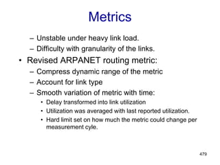
477. 477
Shortest Path Routing
1.Bellman-Ford Algorithm [Distance Vector]
2.Dijkstra’s Algorithm [Link State]
What does it mean to be the shortest (or
optimal) route?
Choices:
a.Minimize the number of hops along the
path.
b.Minimize mean packet delay.
c.Maximize the network throughput.

478. 478
Metrics
• Set all link costs to 1.
– Shortest hop routing.
– Disregards delay.
• Measure the number of packets queued.
– Did not work well.
• Timestamp ArrivalTime and DepartTime*
and use link-level ACK to compute:
Delay = (DepartTime – ArrivalTime) +
TransmissionTime + Latency
* Reset after retransmission

479. 479
Metrics
– Unstable under heavy link load.
– Difficulty with granularity of the links.
• Revised ARPANET routing metric:
– Compress dynamic range of the metric
– Account for link type
– Smooth variation of metric with time:
• Delay transformed into link utilization
• Utilization was averaged with last reported utilization.
• Hard limit set on how much the metric could change per
measurement cyle.

480. 480
Figure 4.22 Revised ARPANET routing metric
versus link utilization
225
140
90
75
60
30
25% 50% 75% 100%
Utilization
9.6-Kbps satellite link
9.6-Kbps terrestrial link
56-Kbps satellite link
56-Kbps terrestrial link
P&D slide

481. 481
Dijkstra’s Shortest Path Algorithm
Initially mark all nodes (except source) with
infinite distance.
working node = source node
Sink node = destination node
While the working node is not equal to the
sink
1. Mark the working node as permanent.
2. Examine all adjacent nodes in turn
If the sum of label on working node plus distance from working node to
adjacent node is less than current labeled distance on the adjacent node,
this implies a shorter path. Relabel the distance on the adjacent node and
label it with the node from which the probe was made.
3. Examine all tentative nodes (not just

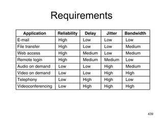
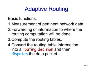
482. 482
Internetwork Routing [Halsall]
Adaptive Routing
Centralized Distributed
Intradomain routing Interdomain routing
Distance Vector routing Link State routing
[IGP] [EGP]
[BGP,IDRP]
[OSPF,IS-IS,PNNI]
[RIP]
[RCC]
Interior
Gateway Protocols
Exterior
Gateway Protocols
Isolated

483. 483
Adaptive Routing
Basic functions:
1.Measurement of pertinent network data.
2.Forwarding of information to where the
routing computation will be done.
3.Compute the routing tables.
4.Convert the routing table information
into a routing decision and then
dispatch the data packet.

484. 484
Adaptive Routing
Design Issues:
1.How much overhead is incurred due to
gathering the routing information and
sending routing packets?
2.What is the time frame (i.e, the
frequency) for sending routing packets
in support of adaptive routing?
3.What is the complexity of the routing
strategy?

485. 485
Distance Vector Routing
• Historically known as the old ARPANET
routing algorithm {or known as Bellman-Ford
algorithm}.
Basic idea: each network node maintains a
Distance Vector table containing the
distance between itself and ALL possible
destination nodes.
• Distances are based on a chosen metric and
are computed using information from the
neighbors’ distance vectors.
Metric: usually hops or delay

486. 486
Distance Vector Routing
Information kept by DV router
1. each router has an ID
2. associated with each link connected to a
router, there is a link cost (static or
dynamic) the metric issue!
Distance Vector Table Initialization
Distance to itself = 0
Distance to ALL other routers = infinity number

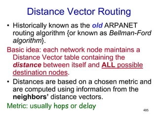
487. 487
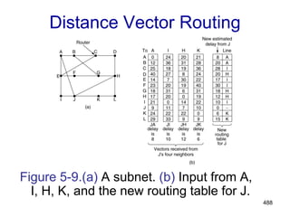
Distance Vector Algorithm
[Perlman]
1.Router transmits its distance vector to each of its
neighbors.
2.Each router receives and saves the most recently
received distance vector from each of its
neighbors.
3.A router recalculates its distance vector when:
a.It receives a distance vector from a neighbor containing
different information than before.
b.It discovers that a link to a neighbor has gone down
(i.e., a topology change).
The DV calculation is based on minimizing the
cost to each destination.

488. 488
Distance Vector Routing
Figure 5-9.(a) A subnet. (b) Input from A,
I, H, K, and the new routing table for J.

489. 489
Routing Information Protocol
(RIP)
• RIP had widespread use because it was
distributed with BSD Unix in “routed”, a router
management daemon.
• RIP is the most used Distance Vector
protocol.
• RFC1058 in June 1988.
• Sends packets every 30 seconds or faster.
• Runs over UDP.
• Metric = hop count
• BIG problem is max. hop count =16
 RIP limited to running on small networks!!
• Upgraded to RIPv2

490. 490
Figure 4.17 RIP Packet Format
Address of net 2
Distance to net 2
Command Must be zero
Family of net 2 Address of net 2
Family of net 1 Address of net 1
Address of net 1
Distance to net 1
Version
0 8 16 31
(network_address,
distance)
pairs
P&D slide

491. 491
Link State Algorithm
1.Each router is responsible for meeting its
neighbors and learning their names.
2.Each router constructs a link state packet (LSP)
which consists of a list of names and cost to reach
each of its neighbors.
3.The LSP is transmitted to ALL other routers.
Each router stores the most recently generated
LSP from each other router.
4.Each router uses complete information on the
network topology to compute the shortest path
route to each destination node.

492. 492
Figure 4.18 Reliable LSP Flooding
(a)
X A
C B D
(b)
X A
C B D
(c)
X A
C B D
(d)
X A
C B D
P&D slide

493. 493
Reliable Flooding
• The process of making sure all the nodes
participating in the routing protocol get a
copy of the link-state information from all the
other nodes.
• LSP contains:
– Sending router’s node ID
– List connected neighbors with the
associated link cost to each neighbor
– Sequence number
– Time-to-live

494. 494
Reliable Flooding
• First two items enable route calculation
• Last two items make process reliable
– ACKs and checking for duplicates is
needed.
• Periodic Hello packets used to
determine the demise of a negihbor
• The sequence numbers are not
expected to wrap around.
– => field needs to be large (64 bits)

495. 495
Open Shortest Path First
(OSPF)
• Provides for authentication of routing
messages.
– 8-byte password designed to avoid
misconfiguration.
• Provides additional hierarchy
– Domains are partitioned into areas.
– This reduces the amount of information
transmitted in packet.
• Provides load-balancing via multiple
routes.

496. 496
Open Shortest Path First
(OSPF)
Area 1
Area 0
Area 3
Area 2
R9
R8
R7
R1
R5
R6
R4
R3
R2
Figure 4.32 A Domain divided into Areas
P&D slide
Backbone
area

497. 497
Open Shortest Path First
(OSPF)
• OSPF runs on top of IP, i.e., an OSPF packet
is transmitted with IP data packet header.
• Uses Level 1 and Level 2 routers
• Has: backbone routers, area border routers,
and AS boundary routers
• LSPs referred to as LSAs (Link State
Advertisements)
• Complex algorithm due to five distinct LSA
types.

498. 498
OSPF Terminology
Internal router :: a level 1 router.
Backbone router :: a level 2 router.
Area border router (ABR) :: a backbone
router that attaches to more than one
area.
AS border router :: (an interdomain router),
namely, a router that attaches to routers
from other ASs across AS boundaries.

499. 499
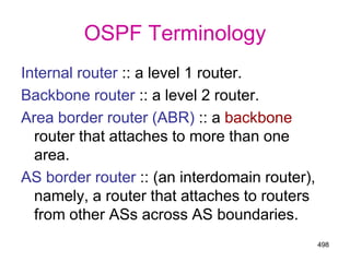
OSPF LSA Types
1.Router link advertisement [Hello
message]
2.Network link advertisement
3.Network summary link advertisement
4.AS border router’s summary link
advertisement
5.AS external link advertisement

500. 500
Figure 4.21 OSF Type 1 Link-State
Advertisement
LS Age Options Type=1
0 Flags 0 Number of links
Link type Num_TOS Metric
Link-state ID
Advertising router
LS sequence number
Link ID
Link data
Optional TOS information
More links
LS checksum Length
P&D slide
Indicates
LSA type
Indicates
link cost

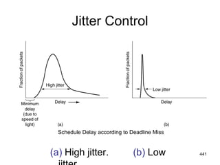
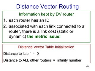
501. 501
Area 0.0.0.1
Area 0.0.0.2
Area 0.0.0.3
R1
R2
R3
R4
R5
R6 R7
R8
N1
N2
N3
N4
N5
N6
N7
To another AS
Area 0.0.0.0
R = router
N =
network
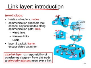
Figure 8.33
Copyright ©2000 The McGraw Hill Companies Leon-Garcia & Widjaja: Communication Networks
OSPF Areas
[AS Border router]
ABR

502. 502
OSPF
Figure 5-65.The relation between
ASes, backbones, and areas in
OSPF.

503. 503
Border Gateway Protocol
(BGP)
• The replacement for EGP is BGP. Current version is
BGP-4.
• BGP assumes the Internet is an arbitrary
interconnected set of AS’s.
• In interdomain routing the goal is to find ANY path to
the intended destination that is loop-free. The
protocols are more concerned with reachability than
optimality.

504. The Transport layer
UNIT-4
504

505. Transport Layer
• Services
• Elements of transport protocol
• Simple transport protocol
• UDP
• Remote Procedure Call (see Distributed
Systems)
• TCP
505

506. Layer overview
application
transport
network
data link
physical
application
transport
network
data link
physical
network
data link
physical
network
data link
physical
network
data link
physical
network
data link
physical
network
data link
physical
506

507. Layer overview
Host 1
Network layer
Application layer
Transport entity
Host 2
Network layer
Application layer
Transport entity
TPDU
Transport
addresses
Network
addresses
507

508. Services
• To upper layer
– efficient, reliable, cost-effective service
– 2 kinds
• Connection oriented
• Connectionless
508

509. Services
• needed from network layer
– packet transport between hosts
– relationship network <> transport
• Hosts <> processes
• Transport service
– independent network
– more reliable
• Network
– run by carrier
– part of communication subnet for WANs
509

510. Simple service: primitives
• Simple primitives:
– connect
– send
– receive
– disconnect
• How to handle incoming connection
request in server process?
Wait for connection request from client!
– listen
510

511. Simple service: primitives
listen Wait till a process wants a connection
connect Try to setup a connection
send Send data packet
receive Wait for arrival of data packet
disconnect Calling side breaks up the connection
No TPDU
Connection Request TPDU
Data TPDU
No TPDU
Disconnect TPDU
511

512. Simple service: state diagram
512

513. Simple service: state diagram
513

514. Simple service: state diagram
514

515. Berkeley service primitives
• Used in Berkeley UNIX for TCP
• Addressing primitives:
• Server primitives:
• Client primitives:
socket
bind
listen
accept
send + receive
close
connect
send + receive
close
515

516. Berkeley service primitives
socket create new communication end point
bind attach a local address to a socket
listen announce willingness to accept connections; give queue size
accept block caller until a connection request arrives
connect actively attempt to establish a connection
send send some data over the connection
receive receive some data from the connection
close release the connection
516

517. Transport Layer
• Services
• Elements of transport protocol
• Simple transport protocol
• UDP
• Remote Procedure Call (see Distributed
Systems)
• TCP
517

518. Elements of transport protocols (etp)
• Transport <> Data Link
• Addressing
• Establishing a connection
• Releasing a connection
• Flow control and buffering
• Multiplexing
• Crash recovery
518

519. etp: Transport <> data link
• Physical channel <> subnet
Explicit addressing
Connection establishment
Potential existence of storage capacity in subnet
Dynamically varying number of connections
519

520. etp: Addressing
• TSAP = transport service access point
– Internet: IP address + local port
– ATM: AAL-SAPs
• Connection scenario
• Getting TSAP addresses?
• From TSAP address to NSAP address?
520

521. etp: Addressing
• Connection scenario
521

522. etp: Addressing
• Connection scenario
– Host 2 (server)
• Time-of-day server attaches itself to TSAP 1522
– Host 1 (client)
• Connect from TSAP 1208 to TSAP 1522
• Setup network connection to host 2
• Send transport connection request
– Host 2
• Accept connection request
522

523. etp: Addressing
• Getting TSAP addresses?
– Stable TSAP addresses
• For key services
• Not for user processes
– active for a short time
– number of addresses limited
– Name servers
• to find existing servers
• map service name into TSAP address
– Initial connection protocol
523

524. etp: Addressing
• Getting TSAP addresses?
– Initial connection protocol
• to avoid many waiting servers  one process
server
– waits on many TSAPs
– creates requested server
524

525. etp: Addressing
• From TSAP address to NSAP address?
– hierarchical addresses
• address = <country> <network> <host> <port>
– Examples: IP address + port
Telephone numbers (<> number portability?)
• Disadvantages:
– TSAP bound to host!
– flat address space
• Advantages:
– Independent of underlying network addresses
– TSAP address not bound to host
• Mapping to network addresses:
– Name server
– broadcast
525

526. etp: Establishing a connection
• Problem: delayed duplicates!
• Scenario:
– Correct bank transaction
• connect
• data transfer
• disconnect
– Problem: same packets are received in same
order a second time!
Recognized?
526

527. etp: Establishing a connection
• Unsatisfactory solutions:
– throwaway TSAP addresses
• need unlimited number of addresses?
• process server solution impossible
– connection identifier
• Never reused!
 Maintain state in hosts
• Satisfactory solutions
527

528. etp: Establishing a connection
• Satisfactory solutions
– Ensure limited packet lifetime (incl. Acks)
– Mechanisms
• prevent packets from looping + bound congestion
delay
• hopcounter in each packet
• timestamp in each packet
– Basic assumption
If we wait a time T after sending a packet all traces
of it (including Acks) are gone
Maximum packet lifetime T
528

529. etp: Establishing a connection
• Tomlinson’s method
– requires: clock in each host
• Number of bits > number of bits in sequence
number
• Clock keeps running, even when a hosts crashes
– Basic idea:
2 identically numbered TPDUs are
never outstanding at the same time!
529

530. etp: Establishing a connection
• Tomlinson’s method
– Problems to solve
• Selection of the initial sequence number for a new
connection
• Wrap around of sequence numbers for an active
connection
• Handle host crashes
Never reuse a sequence number x within
the lifetime T for the packet with x
 Forbidden region
530

531. etp: Establishing a connection
• Tomlinson’s method
– Initial sequence number
= lower order bits of clock
– Ensure initial sequence numbers are always
OK
 forbidden region
– Wrap around
• Idle
• Resynchronize sequence numbers
531

532. etp: Establishing a connection
• Tomlinson - forbidden region
532

533. etp: Establishing a connection
• Tomlinson – three-way-handshake
No combination of
delayed packets can
cause the protocol to fail
533

534. etp: Establishing a connection
• Tomlinson – three-way-handshake
534

535. etp: Releasing a connection
• 2 styles:
– Asymmetric
• Connection broken when one party hangs up
• Abrupt!  may result in data loss
– Symmetric
• Both parties should agree to release connection
• How to reach agreement? Two-army problem
• Solution: three-way-handshake
– Pragmatic approach
• Connection = 2 unidirectional connections
• Sender can close unidirectional connection
535

536. • Asymmetric: data loss
etp: Releasing a connection
536

537. • Symmetric: two-army-problem
etp: Releasing a connection
Simultaneous attack by blue army
Communication is unreliable
No protocol exists!!
537

538. • Three-way-handshake + timers
– Send disconnection request
+ start timer RS to resend (at most N times)
the disconnection request
– Ack disconnection request
+ start timer RC to release connection
etp: Releasing a connection
538

539. etp: Releasing a connection
RC
539

540. etp: Releasing a connection
RS
540

541. etp: Flow control and buffering
Transport Data link
connections, lines many
varying
few
fixed
(sliding) window size varying fixed
buffer management different sizes? fixed size
541

542. etp: Flow control and buffering
• Buffer organization
542

543. etp: Flow control and buffering
• Buffer management: decouple buffering from Acks
543

544. etp: Flow control and buffering
• Where to buffer?
– datagram network  @ sender
– reliable network
+ Receiver process guarantees free buffers?
• No: for low-bandwidth bursty traffic
 @ sender
• Yes: for high-bandwidth smooth traffic
 @ receiver
544

545. etp: Flow control and buffering
• Window size?
– Goal:
• Allow sender to continuously send packets
• Avoid network congestion
– Approach:
• maximum window size = c * r
– network can handle c TPDUs/sec
– r = cycle time of a packet
• measure c & r and adapt window size
545

546. etp: Multiplexing
• Upward: reduce number of network connections to reduce cost
• Downward: increase bandwidth to avoid per connection limits
546

547. etp: Crash recovery
• recovery from network, router crashes?
– No problem
• Datagram network: loss of packet is always handled
• Connection-oriented network: establish new connection + use state to
continue service
• recovery from host crash?
– server crashes, restarts: implications for client?
– assumptions:
• no state saved at crashed server
• no simultaneous events
– NOT POSSIBLE
Recovery from a layer N crash can only
be done by layer N+1 and only if the
higher layer retains enough status
information.
547

548. etp: Crash recovery
• Illustration of problem: File transfer:
– Sender: 1 bit window protocol: states S0, S1
• packet with seq number 0 transmitted; wait for ack
– Receiver: actions
• Ack packet
• Write data to disk
• Order?
548

549. etp: Crash recovery
• Illustration of problem: File transfer
549

550. Transport Layer
• Services
• Elements of transport protocol
• Simple transport protocol
• UDP
• Remote Procedure Call (see Distributed
Systems)
• TCP
550

551. Simple transport protocol
• Service primitives:
– connum = LISTEN (local)
• Caller is willing to accept connection
• Blocked till request received
– connum = CONNECT ( local, remote)
• Tries to establish connection
• Returns identifier (nonnegative number)
– status = SEND (connum, buffer, bytes)
• Transmits a buffer
• Errors returned in status
– status = RECEIVE (connum, buffer, bytes)
• Indicates caller’s desire to get data
– status = DISCONNECT (connum)
• Terminates connection
551

552. • Transport entity
– Uses a connection-oriented reliable network
– Programmed as a library package
– Network interface
• ToNet(…)
• FromNet(…)
• Parameters:
– Connection identifier (connum = VC)
– Q bit: 1 = control packet
– M bit: 1 = more data packets to come
– Packet type
– Pointer to data
– Number of bytes of data
Simple transport protocol
552

553. • Transport entity: packet types
Simple transport protocol
Network packet Meaning
Call request Sent to establish a connection
Call accepted Response to Call Request
Clear Request Sent to release connection
Clear confirmation Response to Clear request
Data Used to transport data
Credit Control packet to manage window
553

554. • Transport entity: state of a connection
Simple transport protocol
State Meaning
Idle Connection not established
Waiting CONNECT done; Call Request sent
Queued Call Request arrived; no LISTEN yet
Established
Sending Waiting for permission to send a packet
Receiving RECEIVE has been done
Disconnecting DISCONNECT done locally
554

555. Simple transport protocol
• Transport entity: code
– See fig 6-20, p. 514 – 517
– To read and study at home!
– Questions?
• Is it acceptable not to use a transport header?
• How easy would it be to use another network
protocol?
555

556. Example Transport Entity (1)
556

557. Example Transport Entity (2)
557

558. Example Transport Entity (3)
558

559. Example Transport Entity (4)
559

560. Example Transport Entity (5)
560

561. Example Transport Entity (6)
561

562. Example Transport Entity (7)
562

563. Example Transport Entity (8)
563

564. Transport Layer
• Services
• Elements of transport protocol
• Simple transport protocol
• UDP
• Remote Procedure Call (see Distributed
Systems)
• TCP
564

565. UDP
• User Data Protocol
– Datagram service between processes
• No connection overhead
– UDP header:
• Ports = identification of end points
565

566. UDP
• Some characteristics
– Supports broadcasting, multicasting
(not in TCP)
– Packet oriented
(TCP gives byte stream)
– Simple protocol
– Why needed above IP?
566

567. Transport Layer
• Services
• Elements of transport protocol
• Simple transport protocol
• UDP
• Remote Procedure Call (see Distributed
Systems)
• TCP
567

568. TCP service model
• point-to-point
– one sender, one receiver
• reliable, in-order byte stream
– no message/packet boundaries
• pipelined & flow controlled
– window size set by TCP congestion and flow control
algorithms
• connection-oriented
– handshaking to get at initial state
• full duplex data
– bi-directional data flow in same connection
568

569. TCP service model
• …
• send & receive buffers
socket
door
TCP
send buffer
TCP
receive buffer
socket
door
segment
application
writes data
application
reads data
569

570. TCP protocol
• Three-way handshake to set up connections
• Every byte has its own 32-bit sequence number
– Wrap around
– 32-bit Acks; window size in bytes
• Segment = unit of data exchange
– 20-byte header + options + data
– Limits for size
• 64Kbyte
• MTU, agreed upon for each direction
– Data from consecutive writes may be accumulated in a single
segment
– Fragmentation possible
• Sliding window protocol
570

571. TCP header
571

572. TCP header
• source & destination ports (16 bit)
• sequence number (32 bit)
• Acknowledgement number (32 bit)
• Header length (4 bits) in 32-bit words
• 6 flags (1 bit)
• window size (16 bit): number of bytes the sender is
allowed to send starting at byte acknowledged
• checksum (16 bit)
• urgent pointer (16 bit) : byte position of urgent data
572

573. TCP header
• Flags:
– URG: urgent pointer in use
– ACK: valid Acknowledgement number
– PSH: receiver should deliver data without delay to user
– RST: reset connection
– SYN: used when establishing connections
– FIN: used to release connection
• Options:
– Maximum payload a host is willing to receive
– Scale factor window size
– Use selective repeat instead of go back n
573

574. TCP connection management
• Three-way handshake
– Initial sequence number: clock based
– No reboot after crash for T (maximum packet lifetime=120 sec)
– Wrap around?
• Connection identification
– Pair of ports of end points
• Connection release
– Both sides are closed separately
– No response to FIN: release after 2*T
– Both sides closed: wait for time 2 * T
574

575. TCP connection management
575

576. 576

577. TCP connection management
State Description
Closed No connection is active or pending
Listen The server is waiting for an incoming call
SYN rcvd A connection request has arrived; wait for ACK
SYN sent The application has started to open a connection
Established The normal data transfer state
FIN wait 1 The application has said it is finished
FIN wait 2 The other side has agreed to release
Timed wait Wait for all packets to die off
Closing Both sides have tried to close simultaneously
Close wait The other side has initiated a release
Last Ack Wait for all packets to die off
577

578. TCP transmission policy
• Window size decoupled from Acks (ex. next slides)
• Window = 0  no packets except for
– Urgent data
– 1 byte segment to send Ack & window size
• Incoming user data may be buffered
– May improve performance: less segments to send
• Ways to improve performance:
– Delay acks and window updates for 500 msec
– Nagle’s algorithm
– Silly window syndrome
578

579. TCP transmission policy
579

580. 580

581. TCP transmission policy
• Telnet scenario: interactive editor reacting on each keystroke:
One character typed
 21 byte segment or 41 byte IP packet
 (packet received) 20 byte segment with Ack
 (editor has read byte) 20 byte segment with window update
 (editor has processed byte; sends echo) 21 byte segment
 (client gets echo) 20 byte segment with Ack
• Solutions:
– delay acks + window updates for 500 msec
– Nagle’s algorithm:
• Receive one byte from user; send it in segment
• Buffer all other chars till Ack for first char arrives
• Send other chars in a single segment
• Disable algorithm for X-windows applications (do not delay sending of mouse
movements)
581

582. • Silly window syndrome
– Problem:
• Sender transmits data in large blocks
• Receiver reads data 1 byte at a time
– Scenario: next slide
– Solution:
• Do not send window update for 1 byte
• Wait for window update till
– Receiver can accept MTU
– Buffer is half empty
TCP transmission policy
582

583. TCP transmission policy
583

584. TCP transmission policy
• General approach:
– Sender should not send small segments
• Nagle: buffer data in TCP send buffer
– Receiver should not ask for small segments
• Silly window: do window updates in large units
584

585. Principles of Congestion Control
Congestion:
• informally: “too many sources sending too much data
too fast for network to handle”
• different from flow control!
= end-to-end issue!
• manifestations:
– lost packets (buffer overflow at routers)
– long delays (queue-ing in router buffers)
• a top-10 problem!
585

586. Causes/costs of congestion: scenario
• two senders, two
receivers
• one router, infinite
buffers
• no retransmission
• large delays
when congested
• maximum
achievable
throughput
586

587. Approaches towards congestion control
end-to-end congestion
control:
• no explicit feedback from
network
• congestion inferred from
end-system observed
loss, delay
• approach taken by TCP
Network-assisted
congestion control:
• routers provide feedback to
end systems
– single bit indicating
congestion (SNA, ATM)
– explicit rate sender
should send at
Two broad approaches towards congestion control:
587

588. TCP Congestion Control
• How to detect congestion?
• Timeout caused by packet loss: reasons
– Transmission errors
– Packed discarded at congested router
: Rare
Packet loss
Hydraulic example illustrating two limitations
for sender!
for wired networks
588

589. TCP congestion control
589

590. TCP Congestion Control
• How to detect congestion?
• Timeout caused by packet loss: reasons
– Transmission errors
– Packed discarded at congested router
: Rare
Packet loss  congestion
Approach: 2 windows for sender
Receiver window
Congestion window
Minimum of 
590

591. TCP Congestion Control
• end-end control (no network assistance)
• transmission rate limited by congestion window size, Congwin,
over segments:
 w segments, each with MSS bytes sent in one RTT:
throughput =
w * MSS
RTT
Bytes/sec
Congwin
591

592. TCP Congestion Control:
• two “phases”
– slow start
– congestion avoidance
• important variables:
– Congwin
– threshold: defines
threshold between two
phases:
• slow start phase
• congestion control phase
• “probing” for usable
bandwidth:
– ideally: transmit as fast as
possible (Congwin as large
as possible) without loss
– increase Congwin until loss
(congestion)
– loss: decrease Congwin,
then begin probing
(increasing) again
592

593. TCP Slow start
• exponential increase (per RTT) in
window size (not so slow!)
• loss event: timeout (Tahoe TCP)
and/or three duplicate ACKs
(Reno TCP)
initialize: Congwin = 1
for (each segment ACKed)
Congwin++
until (loss event OR
CongWin > threshold)
Slow start algorithm
Host A
RTT
Host B
time
593

594. TCP Congestion Avoidance
/* slowstart is over */
/* Congwin > threshold */
Until (loss event) {
every w segments ACKed:
Congwin++
}
threshold = Congwin/2
Congwin = 1
perform slowstart
Congestion avoidance
1
1: TCP Reno skips slowstart (fast
recovery) after three duplicate ACKs
594

595. TCP congestion control
595

596. TCP timer management
• How long should the timeout interval be?
– Data link: expected delay predictable
– Transport: different environment; impact of
• Host
• Network (routers, lines)
unpredictable
• Consequences
– Too small: unnecessary retransmissions
– Too large: poor performance
• Solution: adjust timeout interval based on continuous measurements of
network performance
596

597. TCP timer management
Data link layer Transport layer
597

598. TCP timer management
• Algorithm of Jacobson:
– RTT = best current estimate of the round-trip time
– D = mean deviation (cheap estimator of the standard
variance)
– 4?
• Less than 1% of all packets come in more than 4
standard deviations late
• Easy to compute
Timeout = RTT + 4 * D
598

599. TCP timer management
• Algorithm of Jacobson:
– RTT = a RTT + (1 -a) M a = 7/8
M = last measurement of round-trip time
– D = a D + (1 - a) RTT - M
• Karn’s algorithm: how handle retransmitted segments?
– Do not update RTT for retransmitted segments
– Double timeout
Timeout = RTT + 4 * D
599

600. TCP timer management
• Other timers:
– Persistence timer
• Problem: lost window update packet when window is 0
• Sender transmits probe; receivers replies with window size
– Keep alive timer
• Check whether other side is still alive if connection is idle for
a long time
• No response: close connection
– Timed wait
• Make sure all packets are died off when connection is closed
• = 2 T
600

601. Wireless TCP & UDP
• Transport protocols
– Independent of underlying network layer
– BUT: carefully optimized for wired networks
– Assumption:
• Packet loss caused by congestion
• Invalid for wireless networks: always loss of packets
• Congestion algorithm:
– Timeout ( = congestion)  slowdown
• Solution for wireless networks:
– Retransmit asap
Wireless: Lower throughput – same loss  NO solution
601

602. Wireless TCP
• Heterogeneous networks
• Solutions?
– Retransmissions can cause congestion in wired
network
602

603. Wireless TCP
• Solutions for heterogeneous networks
– Indirect TCP
+ 2 homogeneous connections
– violates TCP semantics
603

604. Wireless TCP
• Solutions for heterogeneous networks
– Snooping agent at base station
• Cashes segments for mobile host
• Retransmits segment if ack is missing
• Removes duplicate acks
• Generates selective repeat requests for segments originating
at mobile host
Snooping
agent
604

605. Wireless UDP
• UDP = datagram service  loss permitted
no problems?
• Programs using UDP expect it to be
highly reliable
• Wireless UDP: far from perfect!!!
Implications for programs recovering from lost
UDP messages
605

606. Transactional TCP
• How to implement RPC?
– On top of UDP?
– Yes if
• Request and reply fit in a single packet
• Operations are idempotent
– Otherwise
• Reimplementation of reliability
– On top of TCP?
606

607. Transactional TCP
How to implement RPC?
• On top of UDP?
– Yes if
• Request and reply fit in a single
packet
• Operations are idempotent
– Otherwise
• Reimplementation of reliability
• On top of TCP?
– Unattractive because of connection
set up
• Solution: transactional TCP
607

608. Transactional TCP
How to implement RPC?
• On top of UDP?
– Problems withreliability
• On top of TCP?
– Overhead of connection set up
• Solution: transactional TCP
– Allow data transfer during setup
– Immediate close of stream
608

609. UNIT 5
INTRODUCTION TO
APPLICATION LAYER
609

610. Chapter 2: Application layer
• 2.1 Principles of network applications
• 2.2 Web and HTTP
• 2.3 FTP
• 2.4 Electronic Mail
– SMTP, POP3, IMAP
• 2.5 DNS
• 2.6 P2P applications
• 2.7 Socket programming with TCP
• 2.8 Socket programming with UDP
610

611. Processes communicating
Process:
program running within a host
Client process:
initiates communication
Server process:
waits to be contacted
process sends/receives messages to/from its socket
identifier includes both IP address and port numbers
associated with process on host.
process
TCP with
buffers,
variables
socket
host or
server
process
TCP with
buffers,
variables
socket
host or
server
Internet
Controlled by OS
controlled by
app developer
611

612. App-layer protocol defines
• Types of messages exchanged,
– e.g., request, response
• Message syntax:
– what fields in messages & how fields are delineated
• Message semantics
– meaning of information in fields
• Rules for when and how processes send & respond to
messages
Public-domain protocols: Proprietary protocols:
 defined in RFCs  e.g., Skype
 allows for interoperability
 e.g., HTTP, SMTP
612

613. Transport service requirements of common apps
Application
file transfer
e-mail
Web documents
real-time audio/video
stored audio/video
interactive games
instant messaging
Data loss
no loss
no loss
no loss
loss-tolerant
loss-tolerant
loss-tolerant
no loss
Throughput
elastic
elastic
elastic
audio: 5kbps-1Mbps
video:10kbps-5Mbps
same as above
few kbps up
elastic
Time Sensitive
no
no
no
yes, 100’s msec
yes, few secs
yes, 100’s msec
yes and no
613

614. Internet transport protocols services
TCP service:
• connection-oriented: setup required between client and server
processes
• reliable transport between sending and receiving process
• flow control: sender won’t overwhelm receiver
• congestion control: throttle sender when network overloaded
• does not provide: timing, minimum throughput guarantees, security
UDP service:
• unreliable data transfer between sending and receiving process
• does not provide: connection setup, reliability, flow control,
congestion control, timing, throughput guarantee, or security
614

615. HTTP overview
PC running
Explorer
Server
running
Apache Web
server
Mac running
Navigator
 Web page consists of base HTML-file
which includes several referenced
objects
 Each object is addressable by a URL
HTTP: hypertext transfer protocol
 Web’s application layer protocol
 client/server model
 client: browser that requests,
receives, “displays” Web objects
 server: Web server sends objects in
response to requests
 uses TCP
 is “stateless”
615

616. HTTP connections
Nonpersistent HTTP
• At most one object is sent
over a TCP connection.
Persistent HTTP
• Multiple objects can be
sent over single TCP
connection between client
and server.
616

617. Non-Persistent HTTP: Response time
Definition of RTT: time for a
small packet to travel from
client to server and back.
Response time:
• one RTT to initiate TCP
connection
• one RTT for HTTP request
and first few bytes of HTTP
response to return
• file transmission time
total = 2RTT+transmit time
time to
transmit
file
initiate TCP
connection
RTT
request
file
RTT
file
received
time time
617

618. Persistent HTTP
Nonpersistent HTTP issues:
• requires 2 RTTs per object
• OS overhead for each TCP connection
• browsers often open parallel TCP connections to fetch referenced
objects
Persistent HTTP
• server leaves connection open after sending response
• subsequent HTTP messages between same client/server sent
over open connection
• client sends requests as soon as it encounters a referenced object
• as little as one RTT for all the referenced objects
618

619. HTTP messages
 two types of HTTP messages: request, response
 HTTP request message:
 ASCII (human-readable format)
619

620. Method types
HTTP/1.0
• GET
– request an object from
server
• POST
– upload information using
forms
• HEAD
– asks server to leave
requested object out of
response
HTTP/1.1
• GET, POST, HEAD
• PUT
– uploads file in entity body
to path specified in URL
field
• DELETE
– deletes file specified in
the URL field
620

621. Cookies: Keeping state
What cookies can bring:
• authorization
• shopping carts
• recommendations
• user session state (Web
e-mail)
Cookies and privacy:
 cookies permit sites to learn a
lot about you
 you may supply name and e-
mail to sites
aside
How to keep “state”:
 protocol endpoints: maintain state at sender/receiver over multiple
transactions
 cookies: http messages carry state
621

622. Web caches (proxy server)
• user sets browser: Web
accesses via cache
• browser sends all HTTP
requests to cache
• Why Web caching?
– reduce response time for
client request
– reduce traffic on an
institution’s access link.
– enables “poor” content
providers to effectively
deliver content
Goal: satisfy client request without involving origin server
client
Proxy
server
client
origin
server
origin
server
622

623. Conditional GET
• Goal: don’t send object if
cache has up-to-date cached
version
• cache: specify date of cached
copy in HTTP request
If-modified-since: <date>
• server: response contains no
object if cached copy is up-to-
date:
HTTP/1.0 304 Not Modified
cache server
HTTP request msg
If-modified-since:
<date>
HTTP response
HTTP/1.0
304 Not Modified
object
not
modified
HTTP request msg
If-modified-since:
<date>
HTTP response
HTTP/1.0 200 OK
<data>
object
modified
623

624. Lecture 5: Outline
• 2.1 Principles of network applications
• 2.2 Web and HTTP
• 2.3 FTP
• 2.4 Electronic Mail
– SMTP, POP3, IMAP
• 2.5 DNS
624

625. FTP: the file transfer protocol
• transfer file to/from remote host
• client/server model
– client: side that initiates transfer (either to/from remote)
– server: remote host
• ftp: RFC 959
• ftp server: port 21
file transfer
FTP
server
FTP
user
interface
FTP
client
local file
system
remote file
system
user
at host
625

626. FTP: separate control, data connections
• FTP client contacts FTP server at
port 21
• client authorized over control
connection
• client browses remote directory by
sending commands over control connection.
• when server receives file transfer command, server opens 2nd TCP
connection (for file) to client
• after transferring one file, server closes data connection.
• server opens another TCP data connection to transfer another file.
• control connection: “out of band”
• FTP server maintains “state”: current directory, earlier authentication
FTP
client
FTP
server
TCP control connection
port 21
TCP data connection
port 20
626

627. FTP commands, responses
Sample commands:
• sent as ASCII text over control channel
• USER username
• PASS password
• LIST return list of file in current directory
• RETR filename retrieves (gets) file
• STOR filename stores (puts) file onto remote host
Sample return codes
• status code and phrase (as in HTTP)
• 331 Username OK, password required
• 125 data connection already open; transfer starting
• 425 Can’t open data connection
• 452 Error writing file 627

628. FTP issues
• Multiple connections are used
– for each directory listing and file transmission
• No integrity check at receiver
• Messages are sent in clear text
– including Passwords and file contents
– can be sniffed by eavesdroppers
• Solution
– Secure FTP (SSH FTP)
• allows a range of operations on remote files
– FTPS ( FTP over Secure Sockets Layer (SSL) )
– Transport Layer Security (TLS) encryption
628

629. Lecture 5: Outline
• 2.1 Principles of network applications
• 2.2 Web and HTTP
• 2.3 FTP
• 2.4 Electronic Mail
– SMTP
– POP3
– IMAP
• 2.5 DNS
629

630. Electronic Mail
Three major components:
• user agents
• mail servers
• simple mail transfer protocol:
SMTP
User Agent
• a.k.a. “mail reader”
• composing, editing, reading
mail messages
• e.g., Eudora, Outlook, elm,
Mozilla Thunderbird
• outgoing, incoming messages
stored on server
user mailbox
outgoing
message queue
mail
server
user
agent
user
agent
user
agent
mail
server
user
agent
user
agent
mail
server
user
agent
SMTP
SMTP
SMTP
630

631. Electronic Mail: mail servers
Mail Servers
• mailbox contains incoming
messages for user
• message queue of outgoing (to
be sent) mail messages
• SMTP protocol between mail
servers to send email messages
– client: sending mail server
– “server”: receiving mail server
mail
server
user
agent
user
agent
user
agent
mail
server
user
agent
user
agent
mail
server
user
agent
SMTP
SMTP
SMTP
631

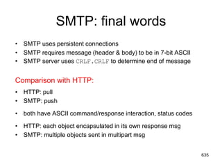
632. Electronic Mail: SMTP [RFC 2821]
• uses TCP to reliably transfer email message from client to
server (port 25)
• direct transfer: sending server to receiving server
• three phases of transfer
– handshaking (greeting)
– transfer of messages
– closure
• command/response interaction
– commands: ASCII text
– response: status code and phrase
• messages must be in 7-bit ASCII
632

633. Scenario: Alice sends message to Bob
1) Alice uses UA to compose message and “to”
bob@someschool.edu
2) Alice’s UA sends message to her mail server; message placed in
message queue
3) Client side of SMTP opens TCP connection with Bob’s mail
server
4) SMTP client sends Alice’s message over the TCP connection
5) Bob’s mail server places the message in Bob’s mailbox
6) Bob invokes his user agent to read message
user
agent
mail
server
mail
server user
agent
1
2 3 4 5
6
633

634. Sample SMTP interaction
S: 220 hamburger.edu
C: HELO crepes.fr
S: 250 Hello crepes.fr, pleased to meet you
C: MAIL FROM: <alice@crepes.fr>
S: 250 alice@crepes.fr... Sender ok
C: RCPT TO: <bob@hamburger.edu>
S: 250 bob@hamburger.edu ... Recipient ok
C: DATA
S: 354 Enter mail, end with "." on a line by itself
C: Do you like ketchup?
C: How about pickles?
C: .
S: 250 Message accepted for delivery
C: QUIT
S: 221 hamburger.edu closing connection
634

635. SMTP: final words
• SMTP uses persistent connections
• SMTP requires message (header & body) to be in 7-bit ASCII
• SMTP server uses CRLF.CRLF to determine end of message
Comparison with HTTP:
• HTTP: pull
• SMTP: push
• both have ASCII command/response interaction, status codes
• HTTP: each object encapsulated in its own response msg
• SMTP: multiple objects sent in multipart msg
635

636. Mail message format
SMTP: protocol for exchanging email msgs
RFC 822: standard for text message format:
• header lines, e.g.,
– To:
– From:
– Subject:
different from SMTP commands!
• body
– the “message”,
ASCII characters only
header
body
blank
line
636

637. Message format: multimedia extensions
• MIME: multimedia mail extension, RFC 2045, 2056
• additional lines in msg header declare MIME content type
From: alice@crepes.fr
To: bob@hamburger.edu
Subject: Picture of yummy crepe.
MIME-Version: 1.0
Content-Transfer-Encoding: base64
Content-Type: image/jpeg
base64 encoded data .....
.........................
......base64 encoded data
multimedia data
type, subtype,
parameter declaration
method used
to encode data
MIME version
encoded data
637

638. Mail access protocols
• SMTP: delivery/storage to receiver’s server
• Mail access protocol: retrieval from server
– POP: Post Office Protocol [RFC 1939]
• authorization (agent <-->server) and download
– IMAP: Internet Mail Access Protocol [RFC 1730]
• more features (more complex)
• manipulation of stored msgs on server
– HTTP: gmail, Hotmail, Yahoo! Mail, etc.
user
agent
sender’s mail
server
user
agent
SMTP SMTP access
protocol
receiver’s mail
server
638

639. POP3 protocol
authorization phase
• client commands:
– user: declare username
– pass: password
• server responses
– +OK
– -ERR
transaction phase, client:
• list: list message numbers
• retr: retrieve message by
number
• dele: delete
• quit
C: list
S: 1 498
S: 2 912
S: .
C: retr 1
S: <message 1 contents>
S: .
C: dele 1
C: retr 2
S: <message 1 contents>
S: .
C: dele 2
C: quit
S: +OK POP3 server signing off
S: +OK POP3 server ready
C: user bob
S: +OK
C: pass hungry
S: +OK user successfully logged on
639

640. POP3 (more) and IMAP
More about POP3
• Previous example uses “download and delete” mode.
• Bob cannot re-read e-mail if he changes client
• “Download-and-keep”: copies of messages on different
clients
• POP3 is stateless across sessions
IMAP
• Keep all messages in one place: the server
• Allows user to organize messages in folders
• IMAP keeps user state across sessions:
– names of folders and mappings between message IDs and
folder name
640

641. Try SMTP interaction for yourself:
• telnet servername 25
• see 220 reply from server
• enter HELO, MAIL FROM, RCPT TO, DATA, QUIT
commands
above lets you send email without using email client
(reader)
641

642. Lecture 5: Outline
• 2.1 Principles of network applications
• 2.2 Web and HTTP
• 2.3 FTP
• 2.4 Electronic Mail
– SMTP
– POP3
– IMAP
• 2.5 DNS
642

643. DNS: Domain Name System
People: many identifiers:
– SSN, name, passport #
Internet hosts, routers:
– IP address (32 bit) - used for addressing datagrams
– “name”, e.g., ww.yahoo.com - used by humans
Domain Name System:
• distributed database implemented in hierarchy of many name
servers
• application-layer protocol host, routers, name servers to
communicate to resolve names (address/name translation)
– note: core Internet function, implemented as application-layer
protocol
– complexity at network’s “edge”
643

644. DNS services
• hostname to IP address translation
• host aliasing
– Canonical, alias names
• mail server aliasing
• load distribution
– replicated Web servers: set of IP addresses for one canonical
name
Why not centralize DNS?
• single point of failure
• traffic volume
• distant centralized database
• maintenance
doesn’t scale!
644

645. Root DNS Servers
com DNS servers org DNS servers edu DNS servers
poly.edu
DNS servers
umass.edu
DNS servers
yahoo.com
DNS servers
amazon.com
DNS servers
pbs.org
DNS servers
Distributed, Hierarchical Database
Client wants IP for www.amazon.com; 1st approx:
• client queries a root server to find com DNS server
• client queries com DNS server to get amazon.com DNS
server
• client queries amazon.com DNS server to get IP
address for www.amazon.com
645

646. Lecture 5: Summary
• Application
• Web and HTTP
• File Transfer Protocol
• Electronic Mail
– SMTP
– POP3
– IMAP
• Domain Name Service
646