non-homogenius differntial equation

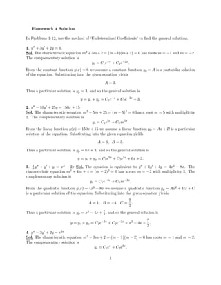
1. Homework 4 Solution
In Problems 1-12, use the method of ‘Undetermined Coefficients’ to find the general solutions.
1. y + 3y + 2y = 6.
Sol. The characteristic equation m2 +3m+2 = (m+1)(m+2) = 0 has roots m = −1 and m = −2.
The complementary solution is
yc = C1e−x
+ C2e−2x
.
From the constant function g(x) = 6 we assume a constant function yp = A is a particular solution
of the equation. Substituting into the given equation yields
A = 3.
Thus a particular solution is yp = 3, and so the general solution is
y = yc + yp = C1e−x
+ C2e−2x
+ 3.
2. y − 10y + 25y = 150x + 15
Sol. The characteristic equation m2 − 5m + 25 = (m − 5)2 = 0 has a root m = 5 with multiplicity
2. The complementary solution is
yc = C1e5x
+ C2xe5x
.
From the linear function g(x) = 150x + 15 we assume a linear function yp = Ax + B is a particular
solution of the equation. Substituting into the given equation yields
A = 6, B = 3.
Thus a particular solution is yp = 6x + 3, and so the general solution is
y = yc + yp = C1e5x
+ C2e5x
+ 6x + 3.
3. 1
4y + y + y = x2 − 2x Sol. The equation is equivalent to y + 4y + 4y = 4x2 − 8x. The
characteristic equation m2 + 4m + 4 = (m + 2)2 = 0 has a root m = −2 with multiplicity 2. The
complementary solution is
yc = C1e−2x
+ C2xe−2x
.
From the quadratic function g(x) = 4x2 − 8x we assume a quadratic function yp = Ax2 + Bx + C
is a particular solution of the equation. Substituting into the given equation yields
A = 1, B = −4, C =
7
2
.
Thus a particular solution is yp = x2 − 4x + 7
2, and so the general solution is
y = yc + yp = C1e−2x
+ C2e−2x
+ x2
− 4x +
7
2
.
4. y − 3y + 2y = e3x
Sol. The characteristic equation m2 − 3m + 2 = (m − 1)(m − 2) = 0 has roots m = 1 and m = 2.
The complementary solution is
yc = C1ex
+ C2e2x
.
1

2. From the exponential function g(x) = e3x we assume an exponential function yp = Ae3x is a
particular solution of the equation. Substituting yp = 3Ae3x and yp = 9Ae9x into the given
equation yields
A =
1
2
.
Thus a particular solution is yp = 1
2e3x, and so the general solution is
y = yc + yp = C1ex
+ C2e2x
+
1
2
e3x
.
5. y − y − 2y = 10 sin x
Sol. The characteristic equation m2 − m − 2 = (m + 1)(m − 2) = 0 has roots m = −1 and m = 2.
The complementary solution is
yc = C1e−x
+ C2e2x
.
From the trig. function g(x) = 10 sin x we try a trig. function yp = A cos x+B sin x for a particular
solution of the equation. Substituting
yp = B cos x − A sin x
yp = −A cos x − B sin x
into the given equation yields
−3A − B = 0, A − 3B = 10.
So we have A = 1 and B = −3. Thus a particular solution is yp = cos x−3 sin x, and so the general
solution is
y = yc + yp = C1e−x
+ C2e2x
+ cos x − 3 sin x.
6. y − 2y − 3y = 6xe2x
Sol. The characteristic equation m2 − 2m − 3 = (m + 1)(m − 3) = 0 has roots m = −1 and m = 3.
The complementary solution is
yc = C1e−x
+ C2e3x
.
From the function g(x) = 6xe2x we try yp = (Ax + B)e2x for a particular solution of the equation.
Substituting
yp = e2x
(2Ax + 2B + A)
yp = e2x
(4Ax + 4B + 2A + 2A)
into the given equation yields
A = −2, B = −4/3
Thus a particular solution is yp = (−2x − 4/3)e2x, and so the general solution is
y = yc + yp = C1e−x
+ C2e3x
+ (−2x − 4/3)e2x
.
7. y + 3y = −48x2e3x
Sol. The characteristic equation m2 + 3 = 0 has complex roots m = ±
√
3i. The complementary
solution is
yc = C1 cos
√
3x + C2 sin
√
3x.
2

3. From the function g(x) = −48x2e3x we try yp = (Ax2 + Bx + C)e3x for a particular solution of the
equation. Substituting
yp = e3x
[3(Ax2
+ Bx + C) + 2Ax + B] = e3x
[3Ax2
+ (2A + 3B)x + B + 3C]
yp = e3x
[3{3Ax2
+ (2A + 3B)x + (B + 3C)} + 6Ax + 2A + 3B] = e3x
[9Ax2
+ (12A + 9B)x + 2A + 6B + 9C]
into the given equation yields
yp + 3yp = e3x
[12Ax2
+ (12A + 12B)x + 2A + 6B + 12]
= e3x
[−48x2
+ 0x + 0].
So we have
A = −4, B = 4 C = −
4
3
.
Thus a particular solution is yp = (−4x2 + 4x − 4
3)e3x, and so the general solution is
y = yc + yp = C1 cos
√
3x + C2 sin
√
3x + (−4x2
+ 4x −
4
3
)e3x
.
8. y − y = −3
Sol. The characteristic equation m2 − m = 0 has two roots m = 0 and m = 1. The complementary
solution is
yc = C1 + C2ex
.
Note that yc already contains constant functions y = A. (One can check y = A can not be a
particular solution of the equation) Instead we modify our assumption and try yp = Ax for a
particular solution of the equation. Substituting yp = A and yp = 0 into the given equation yields
A = 3.
Thus a particular solution is yp = 3x, and so the general solution is
y = yc + yp = C1 + C2ex
+ 3x.
9. y + 2y − 3y = ex
Sol. The characteristic equation m2 + 2m − 3 = (m − 1)(m + 3) = 0 has two roots m = 1 and
m = −3. The complementary solution is
yc = C1ex
+ C2e−3x
.
Note that yc already contains functions y = Aex. Instead we modify our assumption and try
yp = Axex for a particular solution of the equation. Substituting
yp = ex
(Ax + A)
yp = ex
(Ax + A + A)
into the given equation yields
yp + 2yp − 3yp = ex
{(A + 2A − 3A)x + 2A + 2A}
= ex
{ 0x + +1}.
3

4. So we have
A =
1
4
.
Thus a particular solution is yp = 1
4xex, and so the general solution is
y = yc + yp = C1ex
+ C2e−3x
+
1
4
xex
.
10. y − 4y + 4y = e2x
Sol. The characteristic equation m2 − 4m + 4 = (m − 2)2 = 0 has a root m = 2 with multiplicity
2. The complementary solution is
yc = C1e2x
+ C2xe2x
.
Note that yc already contains functions y = Ae2x as well as y = Axe2x. Instead we modify our
assumption and try yp = Ax2e2x for a particular solution of the equation. Substituting
yp = e2x
(2Ax2
+ 2Ax)
yp = e2x
{2(2Ax2
+ 2Ax) + 4Ax + 2A} = e2x
{4Ax2
+ 8Ax + 2A}
into the given equation yields
yp − 4yp + 4yp = e2x
{(4A − 8A + 4A)x2
+ (8A − 8A)x + 2A}
= e2x
{ 0x2
+ 0x + 1}.
So we have
A =
1
2
.
Thus a particular solution is yp = 1
2x2ex, and so the general solution is
y = yc + yp = C1e2x
+ C2xe2x
+
1
2
x2
ex
.
11. y − y + 1
4y = 3 + e
1
2
x
Sol. The characteristic equation m2 − m + 1
4 = (m − 1
2)2 = 0 has a root m = 1
2 with multiplicity
2. The complementary solution is
yc = C1e
1
2
x
+ C2xe
1
2
x
.
In view of Superposition Principle, we seek a particular solution yp = yp1 + yp2 where yp1 and yp2
are particular solutions of
y − y +
1
4
y = 3 and y − y +
1
4
y = ex/2
respectively. As in Problem #1, one can find yp1 = 12.
Note that yc already contains functions y = Ae
1
2
x
as well as y = Axe
1
2
x
. Instead we modify our
assumption and try yp = Ax2e
1
2
x
for a particular solution of the equation. Substituting
yp = e
1
2
x
(
1
2
Ax2
+ 2Ax)
yp = e
1
2
x
{
1
2
(
1
2
Ax2
+ 2Ax) + Ax + 2A} = e
1
2
x
{
1
4
Ax2
+ 2Ax + 2A}
4

5. into the given equation yields
yp − yp +
1
4
yp = e
1
2
x
{(
1
4
A −
1
2
A +
1
4
A)x2
+ (2A − 2A)x + 2A}
= e
1
2
x
{ 0x2
+ 0x + 1}.
So we have
A =
1
2
.
Thus a particular solution is yp = 1
2x2e
1
2
x
, and so the general solution is
y = yc + yp = C1e
1
2
x
+ C2xe
1
2
x
+ 12 +
1
2
x2
e
1
2
x
.
12. y − 8y + 20y = 100x2 − 2 − 13xex
You can use Superposition Principle as discussed during the class.
(or simply yp = Ax2 + Bx + C + (Dx + E)ex also works.)
In Problems 13-16, use the method of ‘Variation of Parameters’ to find the general solutions
13. .y − y − 2y = 2e−x
Sol. The characteristic equation m2 − m − 2 = (m + 1)(m − 2) = 0 has two roots m = 2 and
m = −1. Let y1 = e2x and y2 = e−x. Wronskian W(y1, y2) is
W(y1, y2) =
e2x e−x
2e2x −e−x = −e2x
e−x
− 2e−x
e2x
= −3ex
.
We seek a particular solution yp = u1y1 + u2y2 where u1 =
−y2 · g(x)
W
and u2 =
y1 · g(x)
W
. So
u1 = −
e−x · 2e−x
−3ex
dx =
2
3
e−3x
dx = −
2
9
e−3x
,
u2 =
e2x · 2e−x
−3ex
dx = −
2
3
1dx = −
2
3
x.
Therefore a particular solution is
yp = u1y1 + u2y2 = −
2
9
e−3x
· e2x
−
2
3
x · e−x
= −
2
9
e−x
−
2
3
x · e−x
,
and the the general solution is
y = yc + yp = C1e2x
+ C2e−x
−
2
9
e−x
−
2
3
x · e−x
= C1e2x
+ C2e−x
−
2
3
x · e−x
.
14. y + 2y + y = 3e−x
Sol. The characteristic equation m2 + 2m + 1 = (m + 1)2 = 0 has a root m = −1 with multiplicity
2. Let y1 = e−x and y2 = xe−x. Wronskian W(y1, y2) is
W(y1, y2) =
e−x xe−x
−e−x (1 − x)e−x = e−2x
(1 − x + x) = e−2x
.
5

6. We seek a particular solution yp = u1y1 + u2y2 where u1 =
−y2 · g(x)
W
and u2 =
y1 · g(x)
W
. So
u1 = −
xe−x · 3e−x
e−2x
dx = −3 xdx = −
3
2
x2
,
u2 =
e−x · 3e−x
e−2x
dx = 3 1dx = 3x.
Therefore a particular solution is
yp = u1y1 + u2y2 = −
3
2
x2
· e−x
+ 3x · xe−x
=
3
2
x2
e−x
,
and the the general solution is
y = yc + yp = C1e−x
+ C2xe−x
+
3
2
x2
e−x
15. 4y − 4y + y = 16e
1
2
x
Sol. The standard form of the equation is y − y + 1
4y = 4e
1
2
x
and g(x) = 4e
1
2
x
. The characteristic
equation m2 − m + 1
4 = (m − 1
2)2 = 0 has a root m = 1
2 with multiplicity 2. Let y1 = e
1
2
x
and
y2 = xe
1
2
x
. Wronskian W(y1, y2) is
W(y1, y2) =
e
1
2
x
xe
1
2
x
1
2e
1
2
x
(1 + 1
2x)e
1
2
x
= ex
(1 +
1
2
x −
1
2
x) = ex
.
We seek a particular solution yp = u1y1 + u2y2 where u1 =
−y2 · g(x)
W
and u2 =
y1 · g(x)
W
. So
u1 = −
xe
1
2
x
· 4e
1
2
x
ex
dx = −4 xdx = −2x2
,
u2 =
e
1
2
x
· 4e
1
2
x
ex
dx = 4dx = 4x.
Therefore a particular solution is
yp = u1y1 + u2y2 = −2x2
· e
1
2
x
+ 4x · xe
1
2
x
= 2x2
e
1
2
x
,
and the the general solution is
y = yc + yp = C1e
1
2
x
+ C2xe
1
2
x
+ 2x2
e
1
2
x
16. y + y = sec x
Sol. The characteristic equation m2 + 1 = 0 has complex roots m = ±i. Let y1 = cos x and
y2 = sin x. Wronskian W(y1, y2) is
W(y1, y2) =
cos x sin x
− sin x cos x
= cos2
x + sin2
x = 1.
6

7. We seek a particular solution yp = u1y1 + u2y2 where u1 =
−y2 · g(x)
W
and u2 =
y1 · g(x)
W
. So
u1 = − sin x · sec xdx = −
sin x
cos x
dx = ln | cos x|,
u2 = cos x · sec xdx = cos x ·
1
cos x
dx = 1dx = x.
Therefore a particular solution is
yp = u1y1 + u2y2 = ln | cos x| · cos x + x · sin x,
and the the general solution is
y = yc + yp = C1 cos x + C2 sin x + ln | cos x| cos x + x sin x
In Problems 17-18, solve the given differential equations subject to the initial condition.
17. y + y = 4x + 1, y(0) = 1, y (0) = 4
5
Sol. The characteristic equation m2 + m = m(m + 1) = 0 has roots m = 0 and m = −1. The
complementary solution is
yc = C1e0x
+ C2e−x
= C1 + C2e−x
.
Note that yc and y = Ax + B share constant terms. (One can check the equation does not
have a particular solution of the form y = Ax + B). Instead we modify our assumption and try
yp = x(Ax + B) = Ax2 + Bx for a particular solution of the equation. Substituting yp = 2Ax + B
and yp = 2A into the given equation yields
A = 2, B = −3
Thus a particular solution is yp = x(2x − 3) = 2x2 − 3x, and so the general solution is
y = yc + yp = C1 + C2e−x
+ x(2x − 3).
Since y = −C2e−x + 4x − 3, the initial conditions y(0) = 1, y (0) = 4
5 imply
C1 + C2 = 1 and − C2 − 3 = 4/5.
Now C1 = 24
5 and C2 = −19
5 , and the unique solution is
y =
24
5
−
19
5
e−x
+ x(2x − 3).
18. y + 4y + 5y = 35e−4x, y(0) = −3, y (0) = 1
Sol. The characteristic equation m2+4m+5 = 0 has complex roots m = −2±i. The complementary
solution is
yc = e−2x
(C1 cos x + C2 sin x).
7

8. Our assumption is that yp = Ae−4x is a particular solution for some A. Substituting yp = −4Ae−4x
and yp = 16Ae−4x into the given equation yields
A = 7
Thus a particular solution is yp = 7e−4x, and so the general solution is
y = yc + yp = e−2x
(C1 cos x + C2 sin x) + 7e−4x
.
Since y = e−2x{−2(C1 cos x+C2 sin x)−C1 cos x+C2 cos x}−28e−4x, the initial conditions y(0) =
−3, y (0) = 1 imply
C1 + 7 = −3 and − 2C1 + C2 − 28 = 1.
Now C1 = −10 and C2 = 9, and the unique solution is
y = e−2x
(−10 cos x + 9 sin x) + 7e−4x
.
8