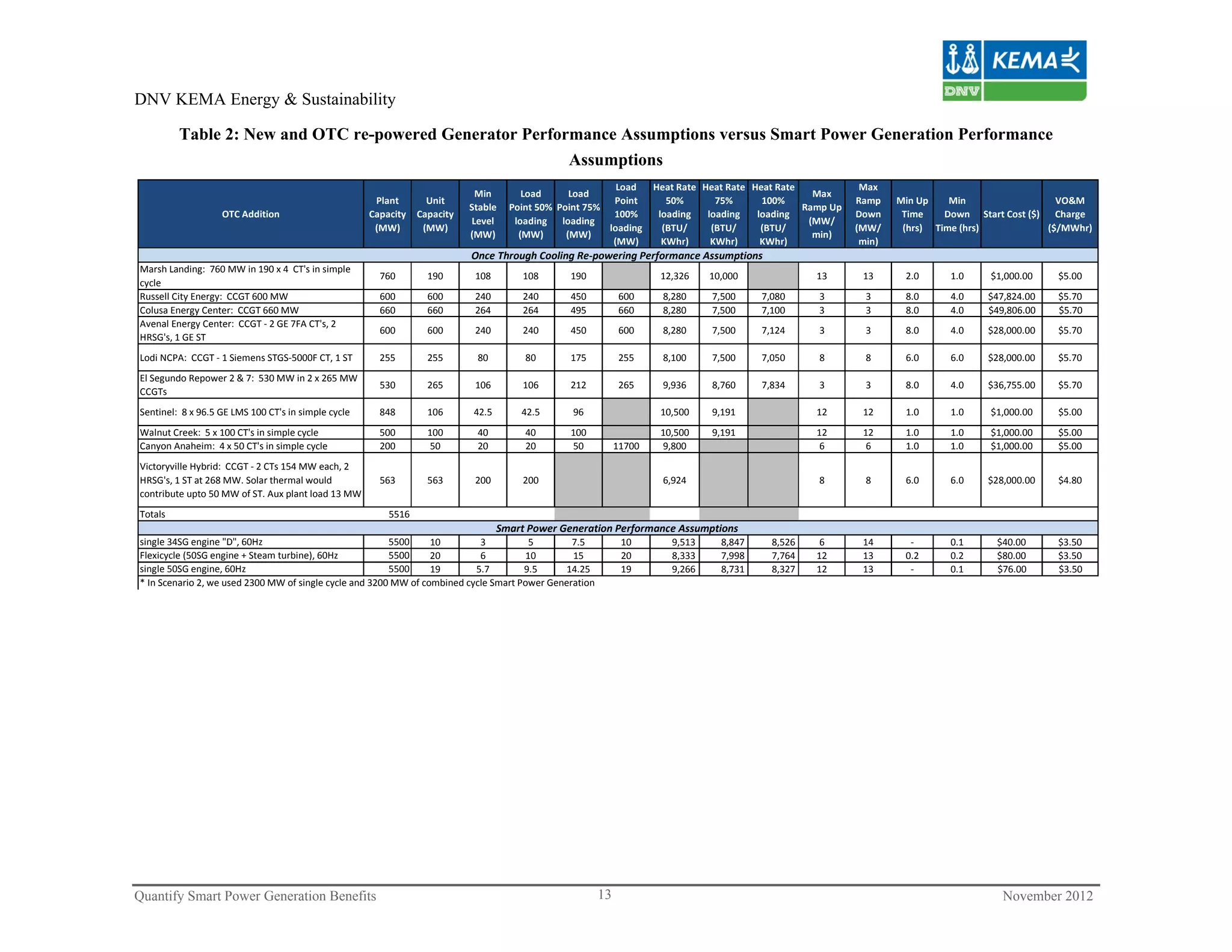
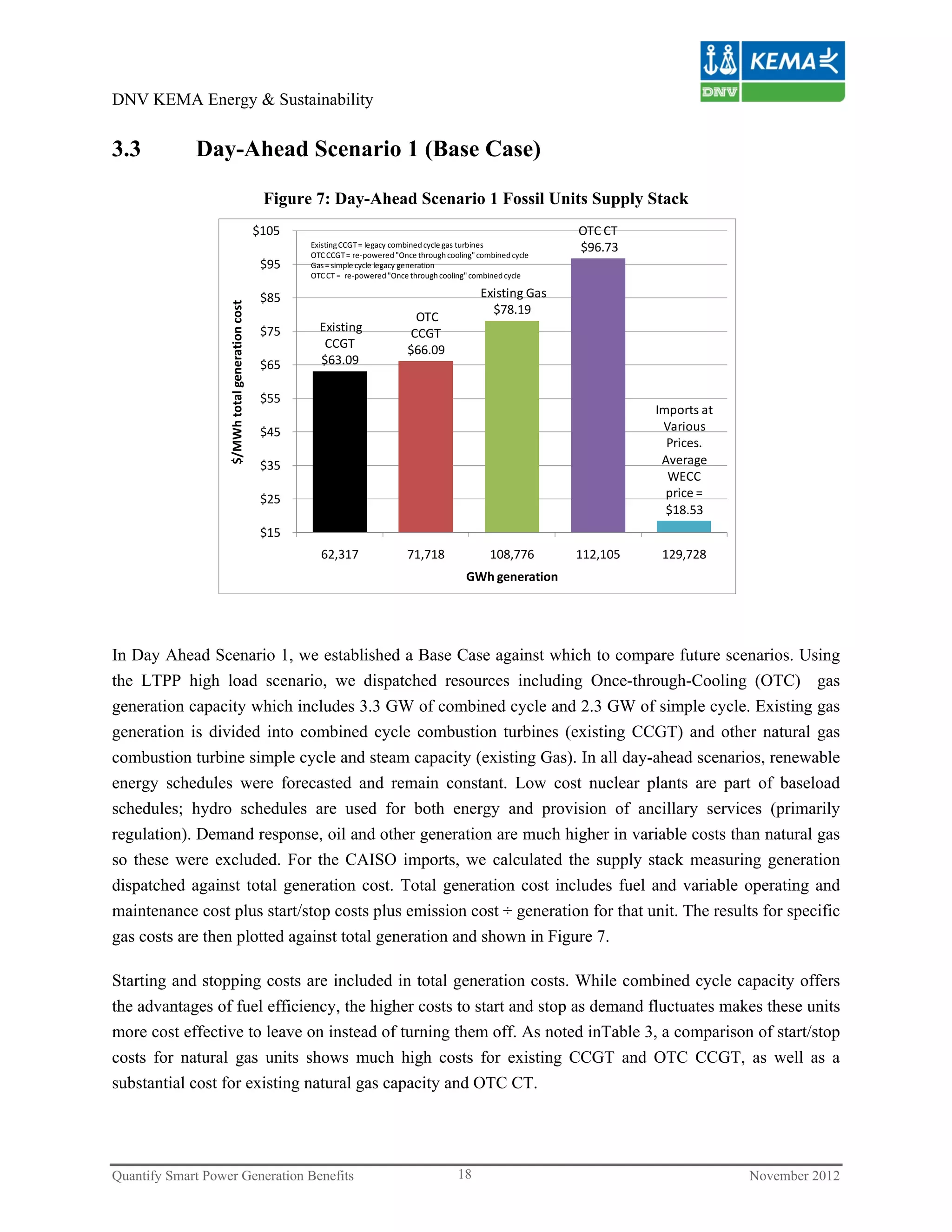
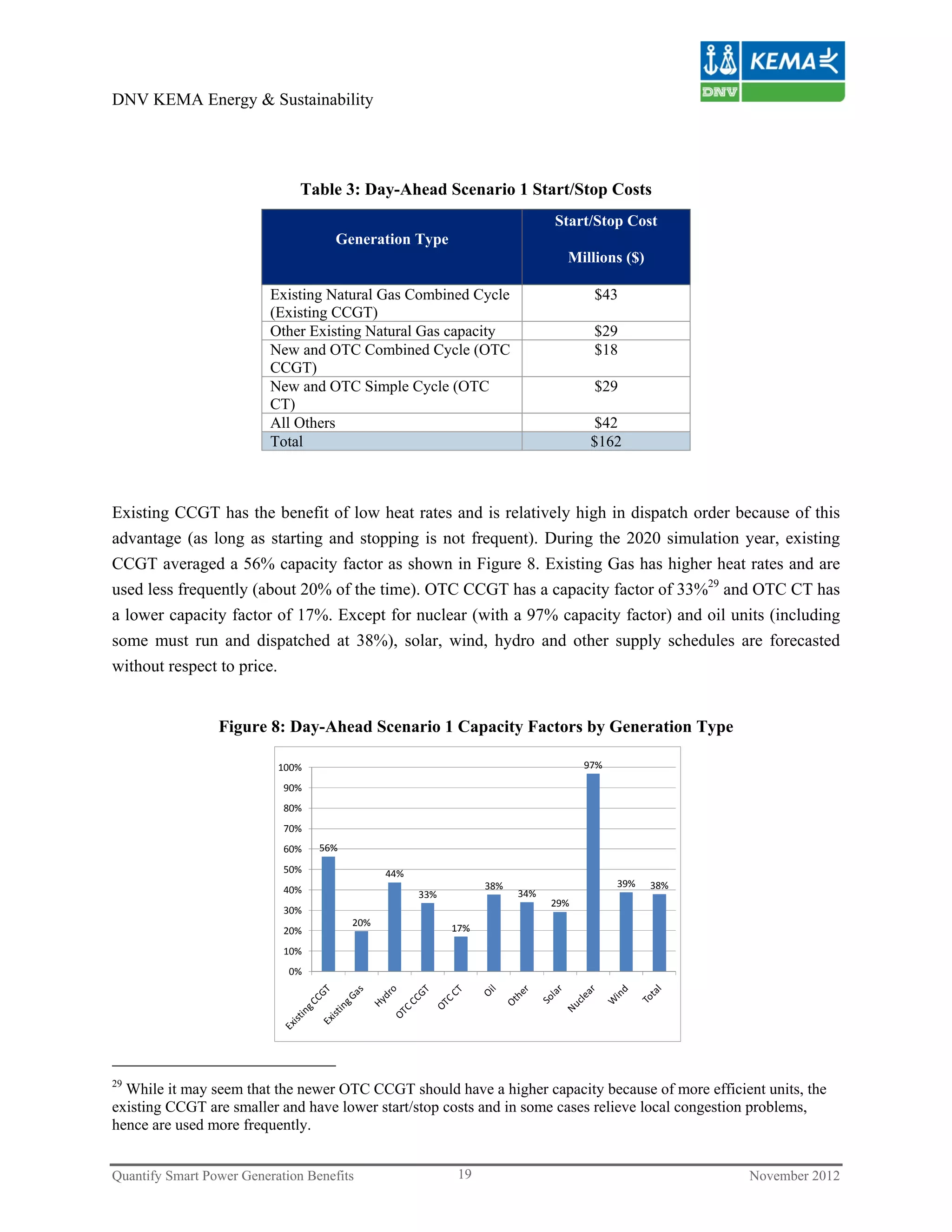
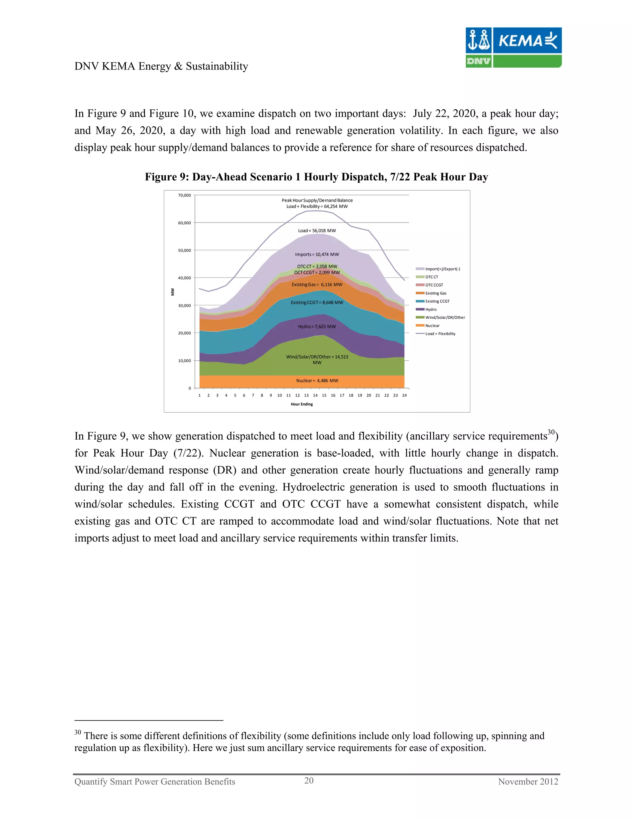
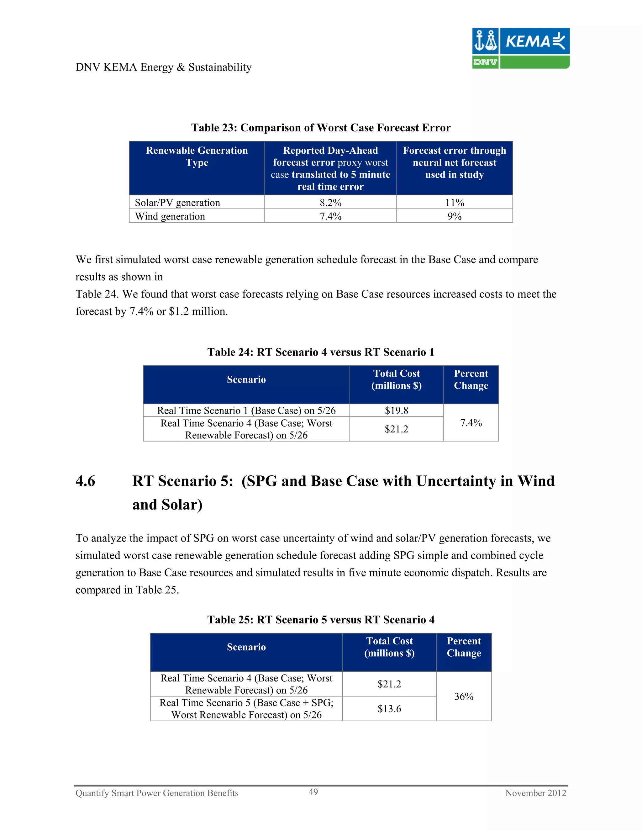
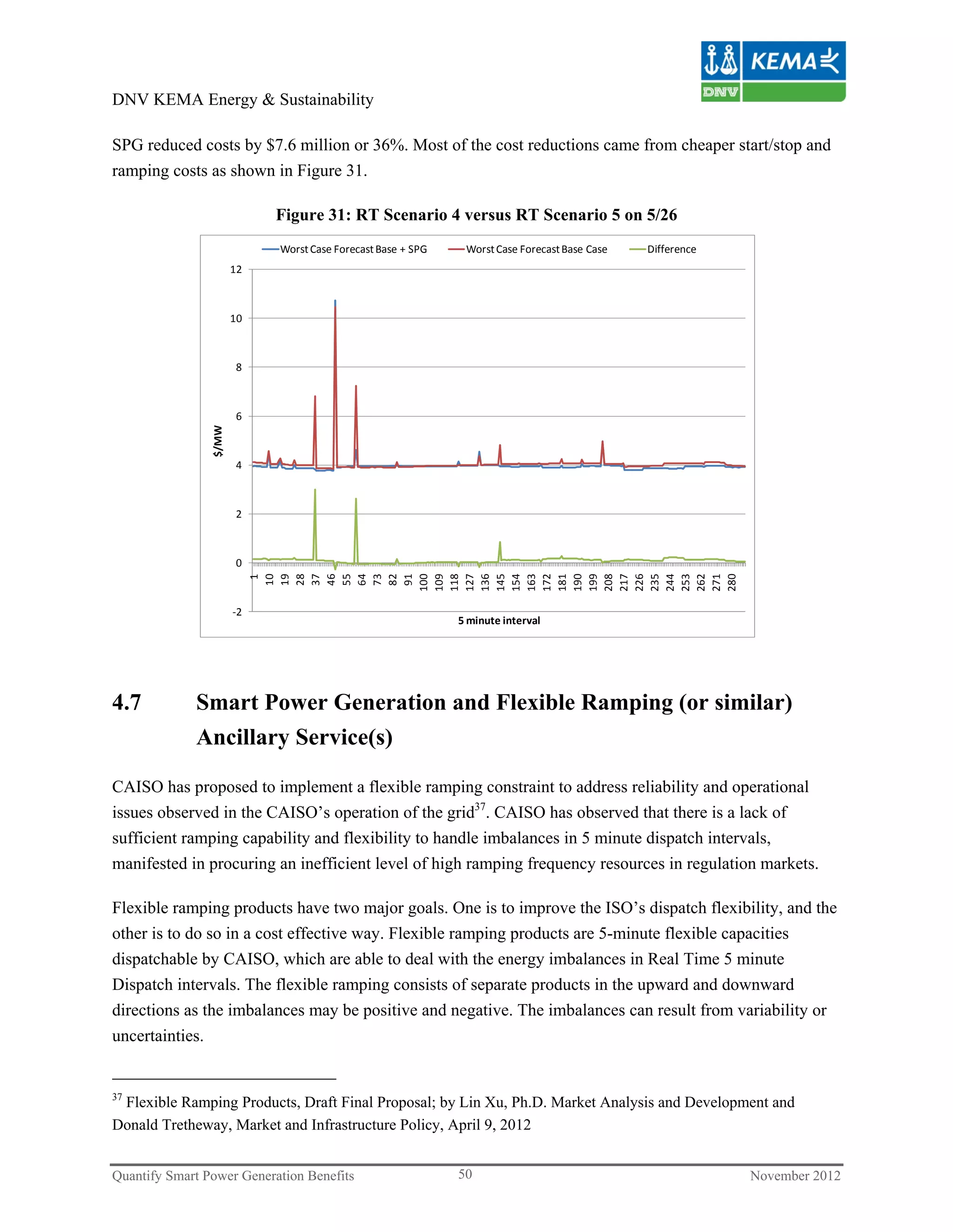
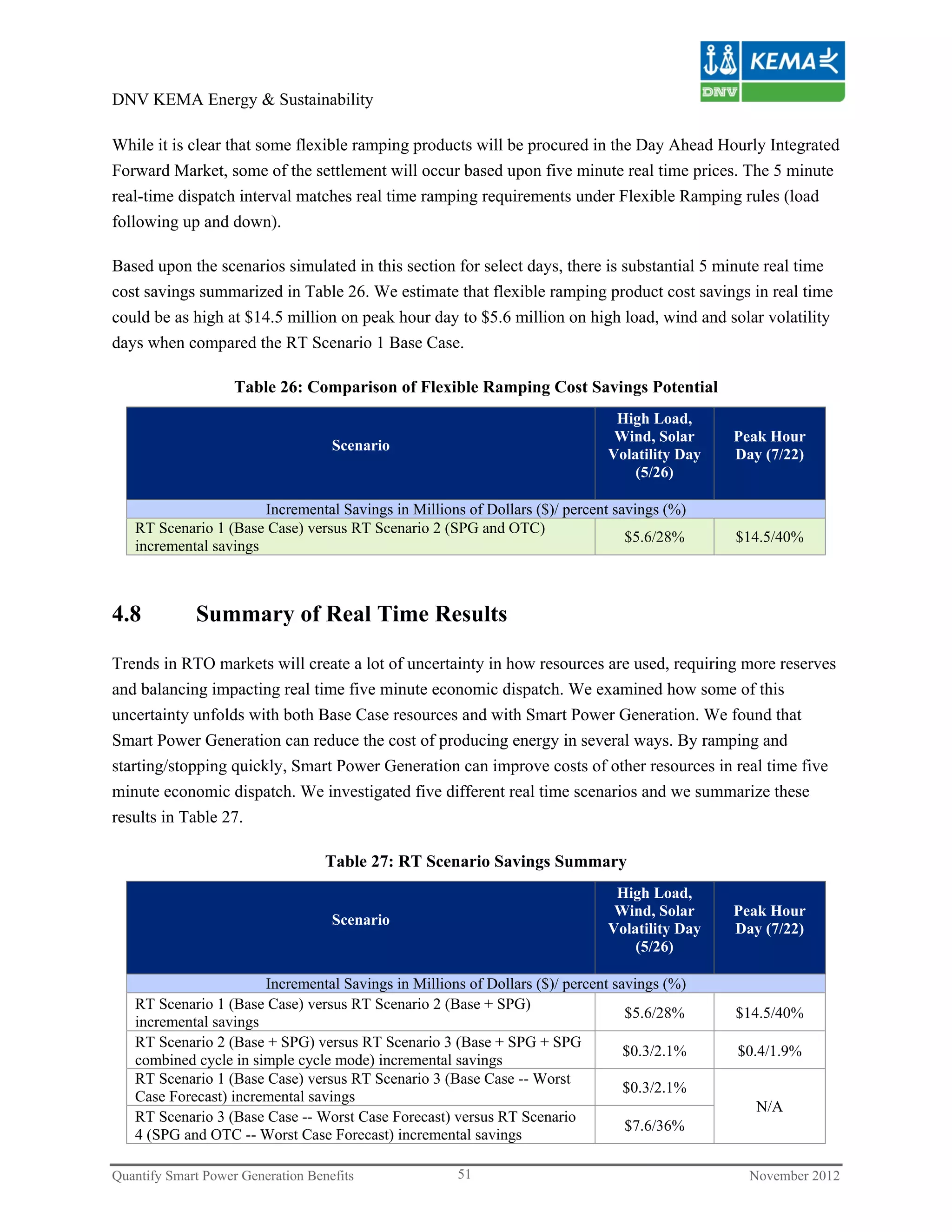
Downloaded 14 times

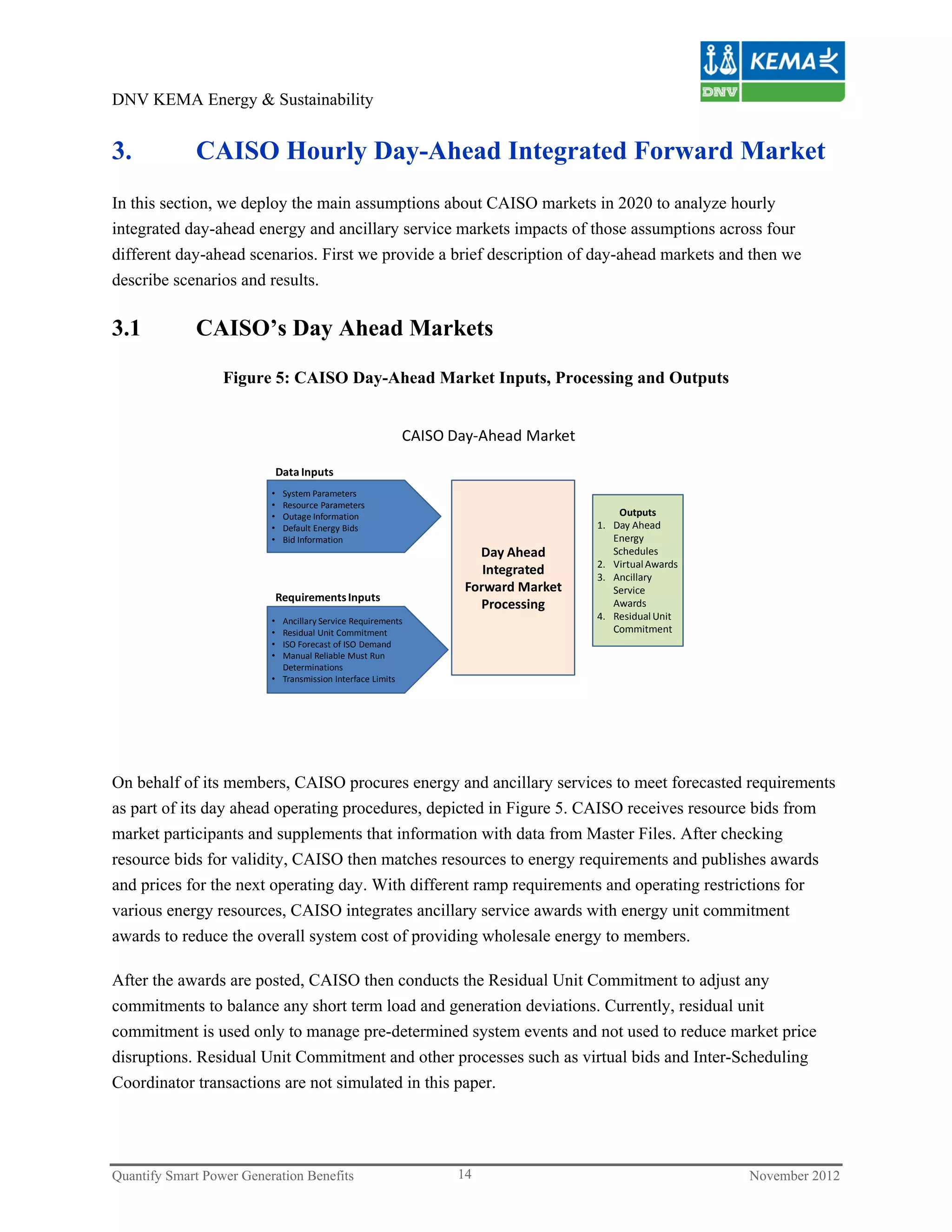
![DNV KEMA Energy & Sustainability
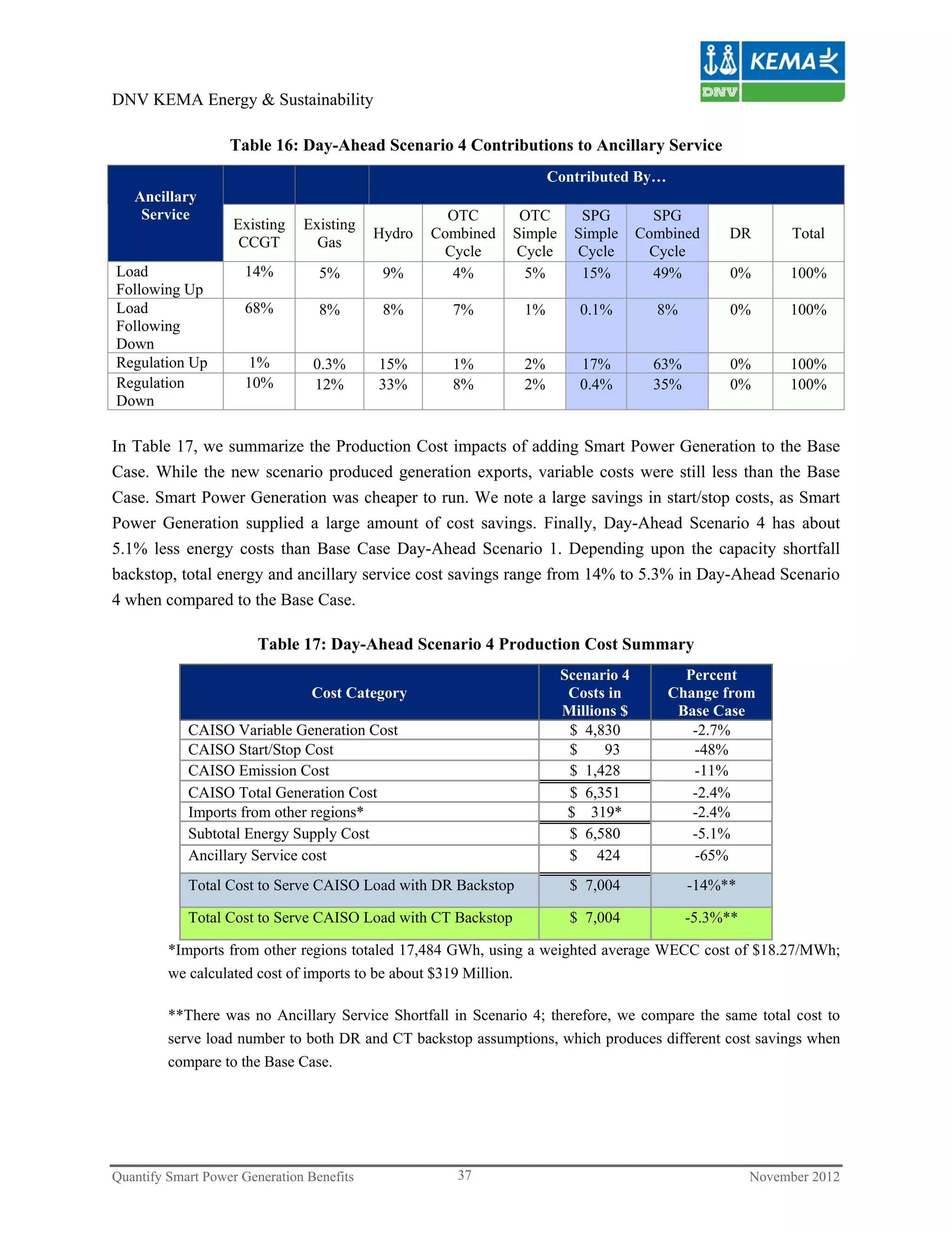
Figure 32: Deliverability @ Risk: Scenario 1 Base Case versus Scenario 4 All Generators
[1] [2] [3] [4] [5] [6] [7] [8]
Scenario 2: Replace Scenario 3: Replace OTC
Scenario 1: OTC with Single with Single & Combined Scenario 4: All
Base Case (1) Cycle Smart Power Cycle Smart Power Generation
Uncertainty Estimate
Resource Generation
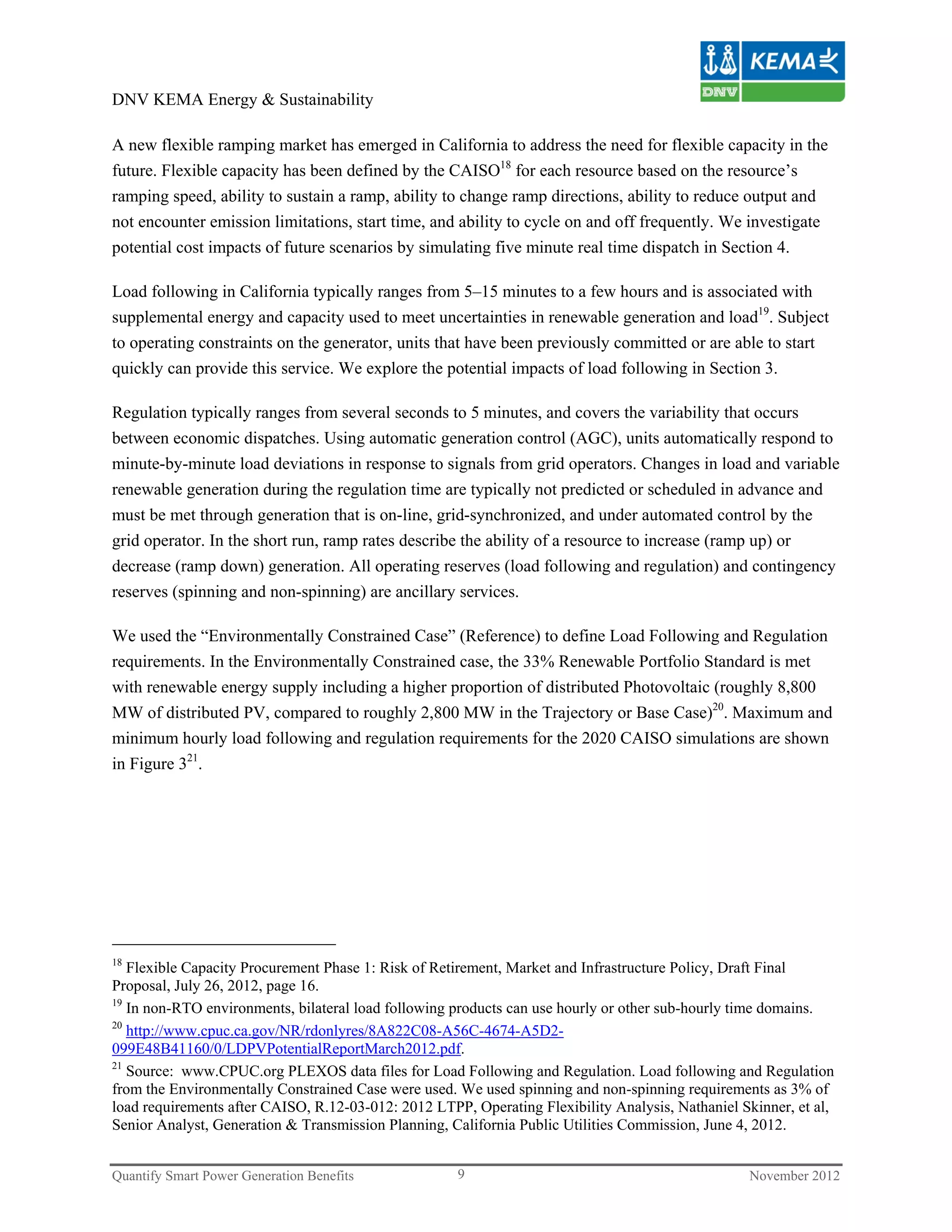
(1)
Generation
(1)
Peak Hour Peak Hour Forced forecast startup ramp rate
Peak Hour Resource Peak Hour Resource
Resource Resource outage error failure variability
MW MW MW MW % % % %
Nuclear
4,486
4,486 4,486
4,486 2% 2%
Other
4,575
3,556 3,556
2,787 5% 1%
Demand Response ‐
‐ ‐
‐ 5% 20% 5% 10%
Solar
8,776
8,776 8,776
8,776 5% 10% 5% 10%
Wind
1,147
1,147 1,147
1,147 5% 10% 5% 10%
Hydro
7,623
8,311 8,306
8,106 6%
Gas 14,764 16,636 16,637
15,795 12% 2%
New OTC Gens
4,157
‐ ‐
4,884 7% 1%
SPG combined cycle) ‐
‐ 2,174
1,875 6% 1%
SPG single cycle ‐
1,593 319
599 6% 1%
Import(+)/Export(‐) 10,474 11,497 10,601
7,562 2%
Smart Power
Generation (single n/a 9,206 9,148 8,683
Smart Power
Generation (combined n/a n/a 9,148 8,683
CT Capacity to Meet 1 d
9,576 n/a n/a 8,794
111
(1) In the Base Case 5.6 GW of repowered OTC generation was used; in Scenario 2, we replaced that generation with Smart Power Generation.
[5] For Gas and New OTC Generation, we used NERC GADS FOR rates. For Demand Response, we used estimates from DNV KEMA's DER estimates. For
[6] Forecast Error measures difference between monitored variable resource and naïve forecast from DNV KEMA's DER estimate.
[7] For Gas, OTC and Wartsila, we used NERC GADS data. For Demand Response, we used DNV KEMA's DER study.
[8] For Demand Response Ramp Rate Variability we used DNV KEMA's DER study.
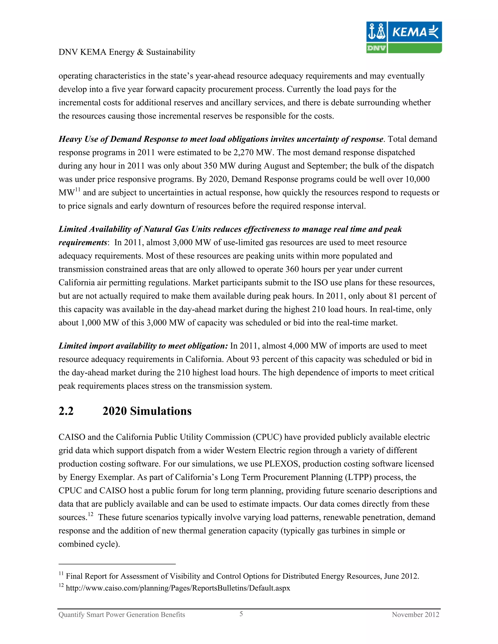
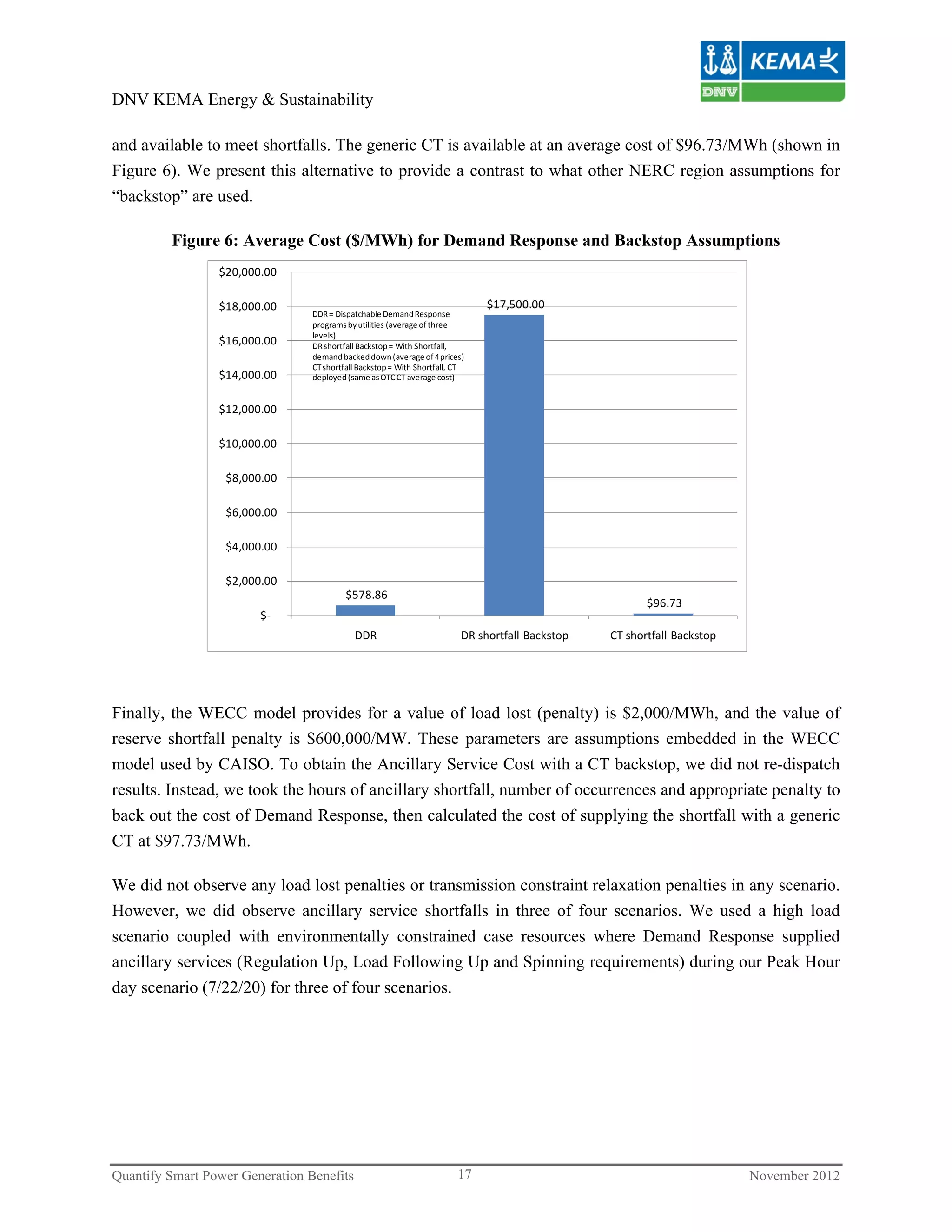
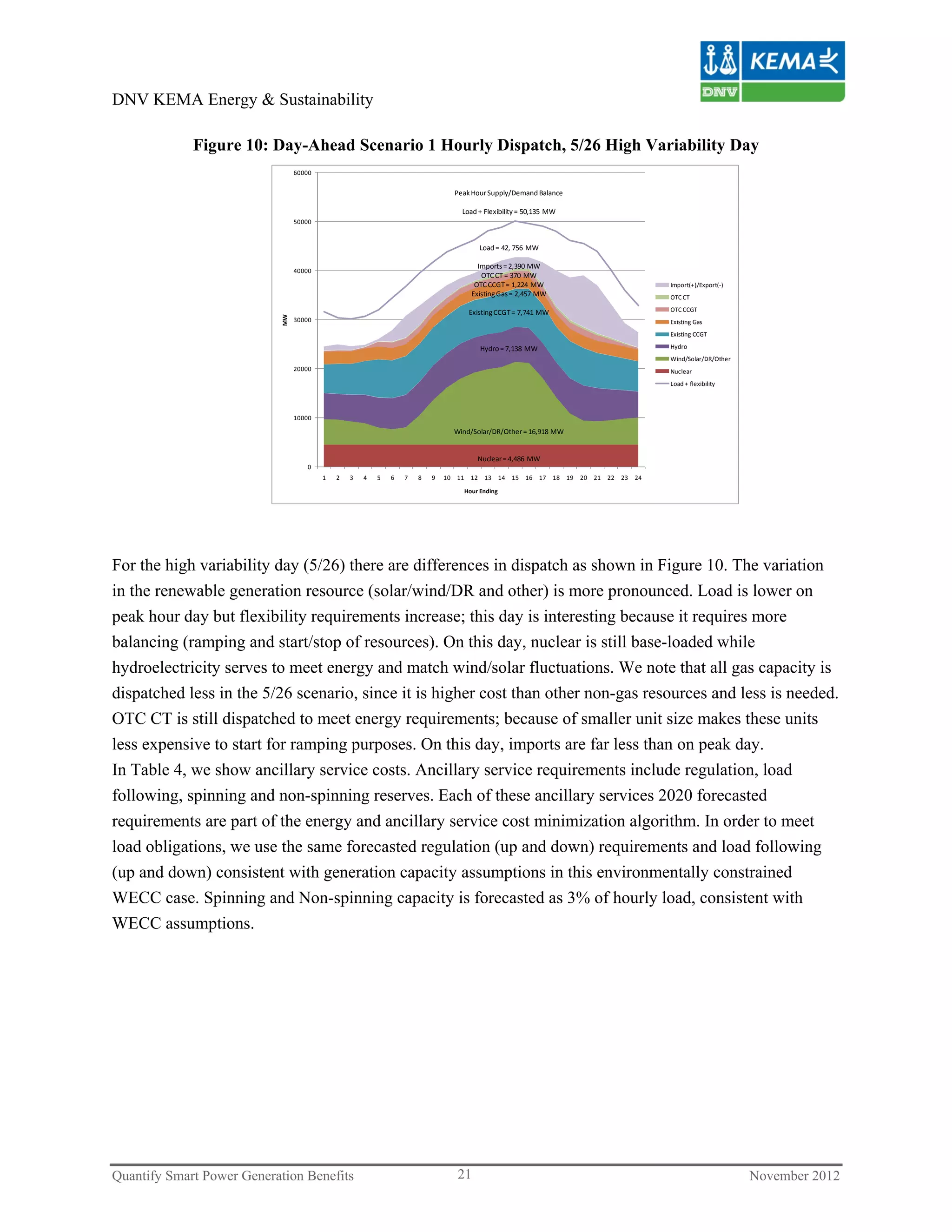
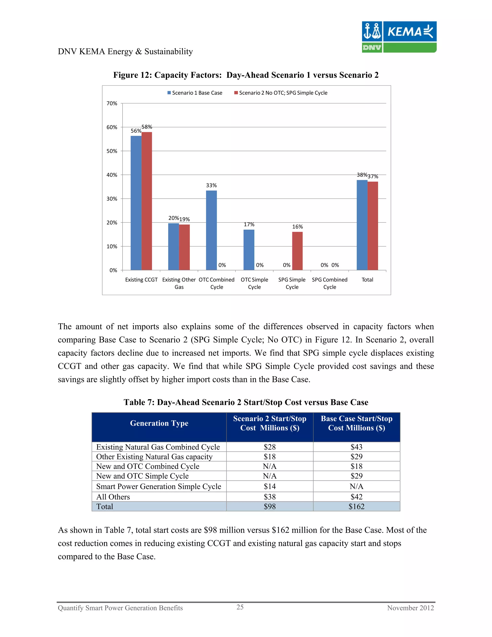
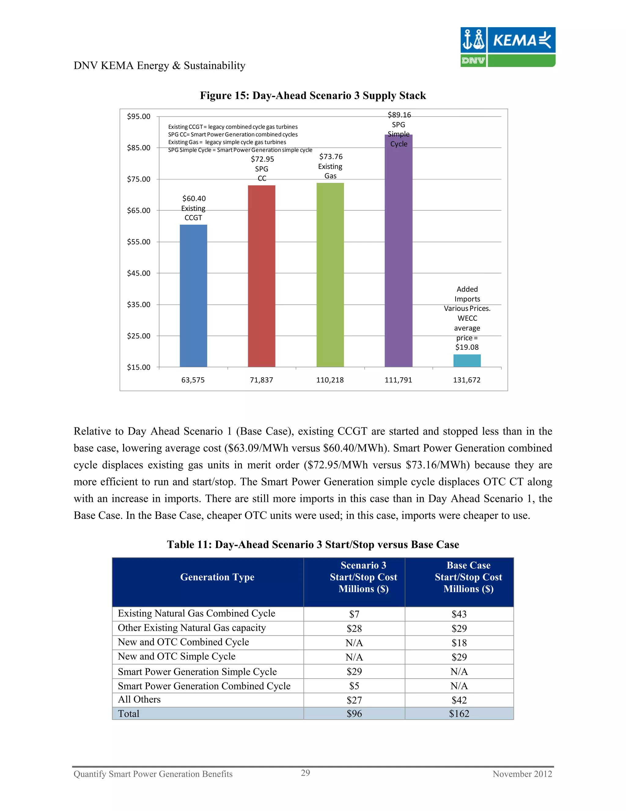
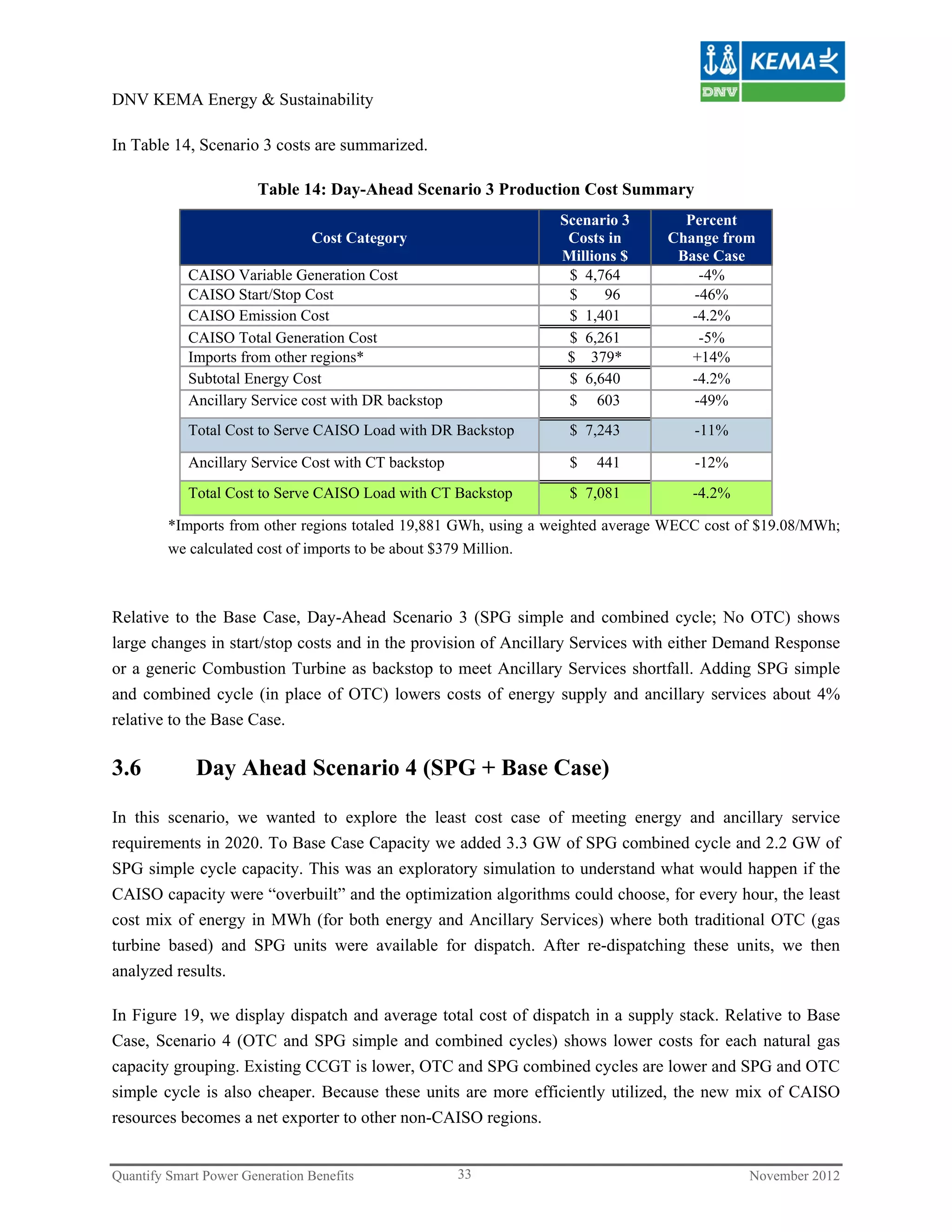
As shown in Figure 32, Demand Response has more uncertainty than most of the fossil generation used in
its place. By reducing the use of demand response, resource adequacy in our scenarios improves. Further,
because Smart Power Generation has less uncertainty than the displaced new or OTC re-powered
generation, less capacity is required to meet the 1 day in 10 years resource adequacy construct.
Relative to the Base Case without Smart Power Generation, Scenario 2 shows that less Smart Power
Generation Capacity is required to meet a one day in ten years resource adequacy criteria (9576 MW
versus 9206 MW).
Relative to the Base Case without Smart Power Generation, Scenario 3 shows that less 50% mix of single
and combined cycle Smart Power Generation Capacity is required to meet a one day in ten years resource
adequacy criteria (9576 MW versus 9148 MW).
Relative to the Base Case without Smart Power Generation, Scenario 4 shows that less 50% mix of single
and combined cycle Smart Power Generation Capacity and new or OTC re-powered generation is
required to meet a one day in ten years resource adequacy criteria (9576 MW versus 8683 or 8794 MW).
Quantify Smart Power Generation Benefits 54 November 2012](https://image.slidesharecdn.com/systemvalueofspgincalifornia2020-130110082719-phpapp02/75/How-to-manage-future-grid-dynamics-system-value-of-Smart-Power-Generation-in-California-in-2020-59-2048.jpg)

The document discusses the dynamics of future electricity grids, focusing on the benefits of smart power generation (SPG) in managing renewable energy integration and ancillary service requirements. It outlines the simulation assumptions for California's electricity market, particularly regarding the California Independent System Operator (CAISO), and evaluates the impact of various SPG scenarios on resource adequacy and operational efficiency. The paper advocates for the use of state-of-the-art combustion engines as a key technology in achieving flexible, efficient, and environmentally responsible energy generation.