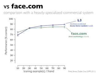
High-Performance Computing Needs
Machine Learning... And Vice Versa
(was “GPU Metaprogramming: A Case Study in Large-Scale Convolutional Neural Networks”)


                                                                                             dit ion
                                                                                         e
Nicolas Pinto
NIPS “Big Learning” | December 16th, 2011


                                                                      The Rowland Institute a
                                                                      HARVARD UNIVERSITY
Outline
1. HPC-aware ML
2. GPU Meta-programming
3. ML-aware HPC
Outline
1. HPC-aware ML
2. GPU Meta-programming
3. ML-aware HPC
Motivation...
The Problem:
Visual Object Recognition
Why?
Why?
it seems easy, right?
44 years ago...
The Problem:
Visual Object Recognition
The Problem:
Visual Object Recognition
The Problem:
Visual Object Recognition

                fast
The Problem:
Visual Object Recognition

                fast
                accurate
The Problem:
Visual Object Recognition

                fast
                accurate
                effortless
The Problem:
Visual Object Recognition

                fast
                accurate
                effortless
                critical to survival
The Problem:
Visual Object Recognition

                fast
                accurate
                effortless
                critical to survival

                tolerant to
                variations!
hard?
hard?


// the world is 3D but the retina is 2D
hard?


// the world is 3D but the retina is 2D
// the curse of dimensionality
hard?


// the world is 3D but the retina is 2D
// the curse of dimensionality

// considerable   image variation
~50% of   is for vision!
you learned it...
      ve
     y ha
   ma
Background
The Approach
Reverse and Forward Engineering the Brain
The Approach
Reverse and Forward Engineering the Brain


     REVERSE                 FORWARD
       Study                       Build
    Natural System            Artificial System
The Approach
Reverse and Forward Engineering the Brain


     REVERSE                 FORWARD
       Study                       Build
    Natural System            Artificial System
Reverse Engineering         Images by DiCarlo JJ & Cox DD
                                        Animation by Li N


The Ventral Visual Stream
Reverse Engineering         Images by DiCarlo JJ & Cox DD
                                        Animation by Li N


The Ventral Visual Stream
Reverse Engineering
The Ventral Visual Stream


                                         taflo ps ?!
                            in =2 0 pe
                      bra
The Approach
Reverse and Forward Engineering the Brain


     REVERSE                 FORWARD
       Study                       Build
    Natural System            Artificial System
Forward Engineering
The Ventral Visual Stream


                                        a rnin g ???
                           a bo ut le
                       all
“Temp. Adv.”
                                                                    “Auto-reset”
                                                                       ...
                                 number of lters


L2
                           thresh/sat            norm strength

                                                            Learning
                                   normalization
                                   neighborhood                      Rate
         kernel                                                      Trace
         size                                                        “Temp. Adv.”
                                                                     “Auto-reset”
                                                                        ...
                                         n. of lters


L1
                  thresh/sat            norm strength            Learning
                                                                      Rate
                                           normalization
                                                                      Trace
                                           neighborhood
                                                                      “Temp. Adv.”
                                                                      “Auto-reset”
kernel                                                                   ...
How are things done normally?

  Usual Formula:
How are things done normally?

  Usual Formula:

  1) One grad student
How are things done normally?

  Usual Formula:

  1) One grad student
  2) One Model (size limited by runtime)
How are things done normally?

  Usual Formula:

  1) One grad student
  2) One Model (size limited by runtime)
  3) Performance numbers on a few
  standard test sets
How are things done normally?

  Usual Formula:

  1) One grad student
  2) One Model (size limited by runtime)
  3) Performance numbers on a few
  standard test sets
  4) yay. we. rock.
How are things done normally?

  Usual Formula:

  1) One grad student
  2) One Model (size limited by runtime)
  3) Performance numbers on a few
  standard test sets
  4) yay. we. rock.
  5) One Ph.D.
How do you call this ?


  “This is graduate student descent”
  - David McAllester
How do you call this ?


  “This is graduate student descent”
  - David McAllester
What’s better than this?


“Conjugate graduate student descent?”
- Nicolas Poilvert
Doing things a little bit differently


  1) One grad student
Doing things a little bit differently


  1) One grad student
  2) One Hundreds of Thousands of
  BIG Models
Doing things a little bit differently


  1) One grad student
  2) One Hundreds of Thousands of
  BIG Models
  3) Performance numbers on a few
  standard test sets
Doing things a little bit differently


  1) One grad student
  2) One Hundreds of Thousands of
  BIG Models
  3) Performance numbers on a few
  standard test sets
Doing things a little bit differently


  1) One grad student
  2) One Hundreds of Thousands of
  BIG Models
  3) Performance numbers on a few
  standard test sets
  4) yay. we. rock.
Doing things a little bit differently


  1) One grad student
  2) One Hundreds of Thousands of
  BIG Models
  3) Performance numbers on a few
  standard test sets
  4) yay. we. rock.
  5) Hundreds of Thousands One PhD ?
“   If you want to have good ideas
         you must have many ideas.               ”
    “  Most of them will be wrong,
      and what you have to learn is
        which ones to throw away.                ”
                    Linus Pauling
                   (double Nobel Prize Winner)
High-throughput
       Screening
Read-out


L3
                  thresh/sat            norm strength

                                            normalization               Learning


                                                                                                  large family of
                                            neighborhood                         Rate
                                                                                 Trace
                                                                                 “Temp. Adv.”
                                                                                 “Auto-reset”

                                               number of lters
                                                                                    ...
                                                                                                  brain-inspired models

L2
                                        thresh/sat            norm strength


                                  clusive!
                                                                         Learning
                                                 normalization
                                                 neighborhood                     Rate


                               in
                                                                                  Trace

                                                                                                    52 parameters
     ery
         kernel
         size                                                                     “Temp. Adv.”


    v
                                                                                  “Auto-reset”
                                                                                     ...
                                                      n. of lters


                                                                                                    more than        10 25
L1
                               thresh/sat            norm strength            Learning


                                                                                                    possible unique
                                                                                   Rate
                                                        normalization
                                                                                   Trace
                                                        neighborhood
                                                                                   “Temp. Adv.”
                                                                                   “Auto-reset”
kernel                                                                                ...


                                                                                                    combinations!
size

                                                                 number of lters


 input
    kernel
    size
                                                                                                         Pinto, Doukhan, DiCarlo, Cox PLoS 2009
The curse of speed
The curse of speed


  thousands of big models
The curse of speed


  thousands of big models

  large amounts of unsupervised
  learning experience
The curse of speed
...and the blessing of massively parallel computing

  No off-the-shelf solution? DIY!
  Engineering (Hardware/SysAdmin/Software)   Science
The curse of speed
...and the blessing of massively parallel computing

  No off-the-shelf solution? DIY!
  Engineering (Hardware/SysAdmin/Software)   Science


  Leverage non-scientific high-tech
  markets and their $billions of R&D...
  Gaming: Graphics Cards (GPUs), PlayStation 3
  Web 2.0: Cloud Computing (Amazon, Google)
r ow n!
 u ild you
B
The blessing of GPUs
  Computational power         DIY GPU pr0n (since 2006)   Sony Playstation 3s (since 2007)


                                                                              GPUs
                        Peak GFLOP/s


                                                                              CPUs
speed
                 (in billion floating point operations per second)


    Q9450 (Matlab/C) [2008]    0.3


        Q9450 (C/SSE) [2008]   9.0


7900GTX (OpenGL/Cg) [2006]           68.2


     PS3/Cell (C/ASM) [2007]            111.4


  8800GTX (CUDA1.x) [2007]                      192.7


   GTX280 (CUDA2.x) [2008]                              339.3


   GTX480 (CUDA3.x) [2010]                                                                      974.3
    (Fermi)
                                                                Pinto, Doukhan, DiCarlo, Cox PLoS 2009
                                                                     Pinto, Cox GPU Comp. Gems 2011
speed
                 (in billion floating point operations per second)


    Q9450 (Matlab/C) [2008]    0.3


        Q9450 (C/SSE) [2008]   9.0


7900GTX (OpenGL/Cg) [2006]           68.2


     PS3/Cell (C/ASM) [2007]            111.4


  8800GTX (CUDA1.x) [2007]                      192.7


   GTX280 (CUDA2.x) [2008]                                  339.3


                                                                             cha n ging...
                                                                         e
   GTX480 (CUDA3.x) [2010]
                                              pe        edu p is g a m                                           974.3
    (Fermi)
                                     >1 000X s
                                                                                 Pinto, Doukhan, DiCarlo, Cox PLoS 2009
                                                                                      Pinto, Cox GPU Comp. Gems 2011
High-throughput Screening
        Skimming off the best models

                          stupid
              chance     baseline
        250


        200
                                         N=2500
        150
Count


        100


        50


         0
               50        60         70   80   90   100


                       Performance (%)                   Pinto, Doukhan, DiCarlo, Cox PLoS 2009
High-throughput Screening
Validate on other tasks

                                                           ~90%
                                   vs.


                   “HMAX 2.1”
                     (~80%)


      V1-like                            5   4    3       2      1
      (baseline)
                   state-of-the-art      high-throughput models
                   (from literature)
                                             Pinto, Doukhan, DiCarlo, Cox PLoS 2009
High-throughput Screening
Validate on faces


                                               vs.


                                               HMAX 2.1
                                 PHOG
                            GB


                                        PHOW
                   SIFT


                                                                                            blend
                                                          5   4        3      2       1
      V1-like                                             high-throughput models
      (baseline)          state-of-the-art
                          (from literature)                       Pinto, Doukhan, DiCarlo, Cox PLoS 2009
Human vs. Machine
  8-way object categorization

                                           99.1


                               64


                  31.3
chance (12.5%)

                 baseline   best model   best human
What does it all mean?
what have we learned ?


                    briefly...
What does it all mean?
what have we learned ?
Grayscale Input
                        Normalize                                        Linear SVM
                                                                       simple classifier


                                          L1         L2           L3

                  Filter
                                    Threshold &
                        Φ1                        Pool    Normalize
                                     Saturate
                        Φ2
                  ...
                        Φk


➡   dimensionality: more filters is better
What does it all mean?
what have we learned ?
Grayscale Input
                        Normalize                                        Linear SVM
                                                                       simple classifier


                                          L1         L2           L3

                  Filter
                                    Threshold &
                        Φ1                        Pool    Normalize
                                     Saturate
                        Φ2
                  ...
                        Φk


➡   learning is difficult
What does it all mean?
what have we learned ?
Grayscale Input
                        Normalize                                        Linear SVM
                                                                       simple classifier


                                          L1         L2           L3

                  Filter
                                    Threshold &
                        Φ1                        Pool    Normalize
                                     Saturate
                        Φ2
                  ...
                        Φk


➡   non-linearities are important
What does it all mean?
what have we learned ?
Grayscale Input
                        Normalize                                        Linear SVM
                                                                       simple classifier


                                          L1         L2           L3

                  Filter
                                    Threshold &
                        Φ1                        Pool    Normalize
                                     Saturate
                        Φ2
                  ...
                        Φk


➡   normalization is very important
    missed in previous modeling efforts
    now confirmed by LeCun et al., Poggio et al., Ng et al.
What are these models
      not good for?
ob jects
 low  level
              s
   ckgr ound
 ba
   fa ces
Outline
1. HPC-aware ML
2. GPU Meta-programming
3. ML-aware HPC
one more thing
Real-world apps?
testing the generality and scalability of the approach
Facebook
Really Real World Problem

                                  enormous scale
                                     billion of photos
                                     3TB+ uploaded
                                     every day
                                     dense, collaborative
                                     face labels


collab. with Zak Stone & Todd Zickler @ Harvard
Relevance to Social Networking


                         slide courtesy of David Cox
Relevance to Social Networking
High-throughput
       Screening
High-Throughput Screening
 Labeled Faces in the Wild (LFW) View 1
  > 30,000 large-scale models (1to3 layers) screened in only 3 days


                   HT L3s (3 layers)                  top 5 models
                                                      LFW view 1 performance


                                   Lea rning!
                         vised
              o Un super
             N


Pinto, Cox (FG 2011)                             Pinto, Stone, Zickler, Cox (CVPR 2011)
Generalization
 Performance on LFW View 2 (hold out)

                       Face Verification Performance (% correct)

                                                               88.1
                                                  86.8
                                   85.3


                   79.4           Wolf et al.
                                 ACCV 2009      Kumar et al.   Ours
                  V1-like        face.com        ICCV 2009     (HT)


Pinto, Cox (FG 2011)
“Facebook100”
typical social network size?


collab. with Zak Stone & Todd Zickler @ Harvard
                                    Pinto, Stone, Zickler, Cox (CVPR 2011)
Auto-tagging
a network of 100 Facebook friends


                             > 86%
                             accurate
                             (w/ 90 training examples)


collab. with Zak Stone & Todd Zickler @ Harvard
                                     Pinto, Stone, Zickler, Cox (CVPR 2011)
vs face.com
comparison with a heavily-specialized commercial system
                                                                     L3
                                                           (hardware-accelerated
                                                           brute-force random model)
Performance (% correct)


                                                            face.com
                                                            V1-likearound)
                                                         (best technology
                                                            (one layer)


                          training example(s) / friend   Pinto, Stone, Zickler, Cox (CVPR 2011)
Conclusion?
Hardware Matters !


       Yann LeCun’s Mac


              picture courtesy of Koray Kavukcuoglu
Outline
1. HPC-aware ML
2. GPU Meta-programming
3. ML-aware HPC
Two conflicting requirements

   The brain is a massively parallel computer
➡ Big models are paralyzingly slow to run


   Neural data only provides weak constraints
➡ Lots of parameters – hard to explore
Two conflicting requirements

   The brain is a massively parallel computer
                   FA  ST slow to run
➡ Big models are paralyzingly


   Neural data only provides weak constraints
➡ Lots of parameters – hard to explore
Two conflicting requirements

   The brain is a massively parallel computer
                   FA  ST slow to run
➡ Big models are paralyzingly


   Neural data only provides weak constraints
                    LEXI BLE
                F
➡ Lots of parameters – hard to explore
Two conflicting requirements

   The brain is a massively parallel computer
                   FA  ST slow to run
➡ Big models are paralyzingly


   Neural data only provides weak constraints
                    LEXI BLE
                F
➡ Lots of parameters – hard to explore


  How to optimize?
What’s the bottleneck?
lutio ns!
                     k Co nvo
       i lter ba n
3D F
Our answer?
Meta-programming

       !
Meta-programming

What?
Meta-programming !


 Leave the grunt-programming to the
 computer (i.e. auto-tuning like ATLAS or FFTW)
 •   Dynamically compile specialized versions
     of the same kernel for different conditions
 •   Empirical run-time tuning
 •   For free: smooth syntactic ugliness: unroll
     loops, index un-indexable registers, etc.
Meta-programming !

“Instrument” your solutions:
•   Block size
•   Work size
•   Loop unrolling
•   Pre-fetching
•   Spilling
•   etc.
                     ... and let the computer generate
                     find the optimal code
How?
Always use the right tool !
texture<float4, 1, cudaReadModeElementType> tex_float4;
__constant__ float constant[$FILTER_D][$FILTER_W][$N_FILTERS];

#define IMUL(a, b) __mul24(a, b)
                                                                plating
                                                             Tem
extern "C" {

#for j in xrange($FILTER_H)

  __global__ void convolve_beta_j${j}(float4 *input, float4 *output)
  {

#set INPUT_BLOCK_W = $BLOCK_W+$FILTER_W-1
    __shared__ float shared_in[$INPUT_BLOCK_W][4+1];

    // -- input/output offsets
    const uint in_idx = (blockIdx.y+$j)*INPUT_W + blockIdx.x*blockDim.x + threadIdx.x;
    const uint out_idx = blockIdx.y*OUTPUT_W + blockIdx.x*blockDim.x + threadIdx.x;
    float4 input_v4;

    // -- load input to shared memory
#for i in xrange($LOAD_ITERATIONS)
#if $i==($LOAD_ITERATIONS-1)
    if((threadIdx.x+$BLOCK_W*$i)<$INPUT_BLOCK_W)
#end if
      {
	   input_v4 = tex1Dfetch(tex_float4, in_idx+$BLOCK_W*$i);
	   shared_in[threadIdx.x+$BLOCK_W*$i][0] = input_v4.x;
	   shared_in[threadIdx.x+$BLOCK_W*$i][1] = input_v4.y;
	   shared_in[threadIdx.x+$BLOCK_W*$i][2] = input_v4.z;
Compilation?
  (with Python-based solutions)
PyCUDA/PyOpenCL (by Andreas Klockner)


  Klöckner, Pinto, Lee, Catanzaro, Ivanov, Fasih (ParCo 2011)
Basic GPU Meta-programming System


                                                      A Case Study
                           GPU  Meta-Programming:
                                                 red Machine Vision
                           in Biologically-Inspi
                                                s]
                           [GPU Computing Gem

                           Pinto N, Cox DD
conv_kernel_4x4x4.cu
conv_kernel_template.cu                                          #include <stdio.h>

                                                                 texture<float4, 1, cudaReadModeElementType> tex_float4;
                                                                 __constant__ float constant[4][4][4];

                                                                 #define IMUL(a, b) __mul24(a, b)
 texture<float4, 1, cudaReadModeElementType> tex_float4;         extern "C" {
 __constant__ float constant[$FILTER_D][$FILTER_W]
 [$N_FILTERS];                                                         __global__ void convolve_beta_j0(float4 *input, float4 *output)
                                                                       {
 #define IMUL(a, b) __mul24(a, b)
 extern "C" {                                                           __shared__ float shared_in[131][4+1];

                                                                        // -- input/output offsets
 #for j in xrange($FILTER_H)                                            const uint in_idx = (blockIdx.y+0)*INPUT_W + blockIdx.x*blockDim.x + threadIdx.x;
                                                                        const uint out_idx = blockIdx.y*OUTPUT_W + blockIdx.x*blockDim.x + threadIdx.x;
   __global__ void convolve_beta_j${j}(float4 *input, float4            float4 input_v4;
 *output)
                                                                        // -- load input to shared memory
   {
                                                                          {
                                                                 	

                input_v4 = tex1Dfetch(tex_float4, in_idx+128*0);
 #set INPUT_BLOCK_W = $BLOCK_W+$FILTER_W-1                       	

                shared_in[threadIdx.x+128*0][0] = input_v4.x;
     __shared__ float shared_in[$INPUT_BLOCK_W][4+1];            	

                shared_in[threadIdx.x+128*0][1] = input_v4.y;
                                                                 	

                shared_in[threadIdx.x+128*0][2] = input_v4.z;
                                                                 	

                shared_in[threadIdx.x+128*0][3] = input_v4.w;
     // -- input/output offsets
                                                                          }
     const uint in_idx = (blockIdx.y+$j)*INPUT_W +                      if((threadIdx.x+128*1)<131)
 blockIdx.x*blockDim.x + threadIdx.x;                                     {
     const uint out_idx = blockIdx.y*OUTPUT_W +                  	

                input_v4 = tex1Dfetch(tex_float4, in_idx+128*1);
 blockIdx.x*blockDim.x + threadIdx.x;                            	

                shared_in[threadIdx.x+128*1][0] = input_v4.x;
                                                                 	

                shared_in[threadIdx.x+128*1][1] = input_v4.y;
     float4 input_v4;
                                                                 	

                shared_in[threadIdx.x+128*1][2] = input_v4.z;
                                                                 	

                shared_in[threadIdx.x+128*1][3] = input_v4.w;
      // -- load input to shared memory                                   }
 #for i in xrange($LOAD_ITERATIONS)                                     __syncthreads();
 #if $i==($LOAD_ITERATIONS-1)
                                                                        // -- compute dot products
      if((threadIdx.x+$BLOCK_W*$i)<$INPUT_BLOCK_W)
                                                                        float v, w;
 #end if
        {                                                               float sum0 = 0;
 	         input_v4 = tex1Dfetch(tex_float4, in_idx+$BLOCK_W*           float sum1 = 0;
 $i);                                                                   float sum2 = 0;
                                                                        float sum3 = 0;
 	         shared_in[threadIdx.x+$BLOCK_W*$i][0] = input_v4.x;
 	         shared_in[threadIdx.x+$BLOCK_W*$i][1] = input_v4.y;          v = shared_in[threadIdx.x+0][0];
 	         shared_in[threadIdx.x+$BLOCK_W*$i][2] = input_v4.z;          w = constant[0][0][0];
 	         shared_in[threadIdx.x+$BLOCK_W*$i][3] = input_v4.w;          sum0 += v*w;
        }                                                               w = constant[0][0][1];
                                                                        sum1 += v*w;
 #end for
                                                                        w = constant[0][0][2];
                                                                        sum2 += v*w;
                                                                        w = constant[0][0][3];
                                                                        sum3 += v*w;
                                                                        v = shared_in[threadIdx.x+1][0];
                                                                        w = constant[0][1][0];
                                                                        sum0 += v*w;
                                                                        w = constant[0][1][1];
                                                                        sum1 += v*w;
                                                                        w = constant[0][1][2];
                                                                        sum2 += v*w;
                                                                        w = constant[0][1][3];
                                                                        sum3 += v*w;
                                                                        v = shared_in[threadIdx.x+2][0];
                                                                        w = constant[0][2][0];
                                                                        sum0 += v*w;
                                                                        w = constant[0][2][1];
                                                                        sum1 += v*w;
conv_kernel_template.cu
 texture<float4, 1, cudaReadModeElementType> tex_float4;
 __constant__ float constant[$FILTER_D][$FILTER_W]
 [$N_FILTERS];

 #define IMUL(a, b) __mul24(a, b)
                                                                 conv_kernel_4x4x4.cu
 extern "C" {

 #for j in xrange($FILTER_H)

   __global__ void convolve_beta_j${j}(float4 *input, float4


                                                                             20 kB
 *output)
   {

 #set INPUT_BLOCK_W = $BLOCK_W+$FILTER_W-1
     __shared__ float shared_in[$INPUT_BLOCK_W][4+1];

     // -- input/output offsets
     const uint in_idx = (blockIdx.y+$j)*INPUT_W +
 blockIdx.x*blockDim.x + threadIdx.x;
     const uint out_idx = blockIdx.y*OUTPUT_W +
 blockIdx.x*blockDim.x + threadIdx.x;
     float4 input_v4;

      // -- load input to shared memory
 #for i in xrange($LOAD_ITERATIONS)
 #if $i==($LOAD_ITERATIONS-1)
      if((threadIdx.x+$BLOCK_W*$i)<$INPUT_BLOCK_W)
 #end if

 	
 $i);
        {
           input_v4 = tex1Dfetch(tex_float4, in_idx+$BLOCK_W*    conv_kernel_8x8x4.cu
 	         shared_in[threadIdx.x+$BLOCK_W*$i][0] = input_v4.x;
 	         shared_in[threadIdx.x+$BLOCK_W*$i][1] = input_v4.y;
 	         shared_in[threadIdx.x+$BLOCK_W*$i][2] = input_v4.z;
 	         shared_in[threadIdx.x+$BLOCK_W*$i][3] = input_v4.w;
        }


                                                                             64 kB
 #end for
Benefits?
Smooth syntactic ugliness
  Manipulations that are not easily
  accessible in CUDA C code:
  • loop unrolling (possibly fine-controlled)
Smooth syntactic ugliness
                            Manipulations that are not easily
                            accessible in CUDA C code:
                            • fine-controlled loop unrolling / jamming
..)

  v = shared_in[threadIdx.x+0][0];
  w = constant[0][0][0];
  sum0 += v*w;
  w = constant[0][0][1];
  sum1 += v*w;
  w = constant[0][0][2];
  sum2 += v*w;
  w = constant[0][0][3];
  sum3 += v*w;
  v = shared_in[threadIdx.x+1][0];
  w = constant[0][1][0];
  sum0 += v*w;
  w = constant[0][1][1];
  sum1 += v*w;
  w = constant[0][1][2];
  sum2 += v*w;
  w = constant[0][1][3];
  sum3 += v*w;
  v = shared_in[threadIdx.x+2][0];
  w = constant[0][2][0];
  sum0 += v*w;
  w = constant[0][2][1];
  sum1 += v*w;
  w = constant[0][2][2];
  sum2 += v*w;
  w = constant[0][2][3];
  sum3 += v*w;
  v = shared_in[threadIdx.x+3][0];
  w = constant[0][3][0];
  sum0 += v*w;
  w = constant[0][3][1];
  sum1 += v*w;
  w = constant[0][3][2];
  sum2 += v*w;
  w = constant[0][3][3];
  sum3 += v*w;
  v = shared_in[threadIdx.x+0][1];
  w = constant[1][0][0];
  sum0 += v*w;
  w = constant[1][0][1];
  sum1 += v*w;
  w = constant[1][0][2];
  sum2 += v*w;
  w = constant[1][0][3];
  sum3 += v*w;
How about #pragma unroll ?
   (why don’t you trust the compiler?)
o t alo ne....
    we are n
              s for S ignal
    Using GPU
             elatio n                        pil   ers
         Corr                     ust com
                            ’t tr
                                                                                                                                                                 itchell
                                                                                                                                                  Daniel A. M


                        Don                     gmen
                                          The Murch


                                        ode fr
                                               a
                                                     ts
                                                    ison Widefi
                                                                 eld Array


                                                                                                                                             c
                                                                                                                                      tical”
                                                                                                                              e “iden
                                                                                                                       re thes                 + g *h;
                                                                                                                   ompa                                                                                  LOPS
                                                                                                        •        C
                                                                                                                  *c +
                                                                                                                                           e*f
                                                                                                                                                                                                  770 GF
                                                                                                              + d
                                                                                                          b*c                       grating 8-s
                                                                                                                                                econd snap
                                                                                                                                                            shots over


                                                                                                     a +=
                                                                                                                               inte                           peeling,
                                                                                                                   roduced by                     lanking and

                                                                                                                     b*c;
                                                                                                   -2 526 field p                    d after RFI b
                                                                                      f the J2107                      e of the fiel
                                                                           an image o                    ht is an imag
                                                                                                                                                                                                        S
                                                                                                                                                                                                    FLOP
                                                             n the left is                  . On the rig

                                                                                                               a += d*c;
                                               Figure 3:
                                                           O                            ing
                                                                             hout blank
                                                                interval wit

                                                                                                                                                                                               20 G
                                                   entire time                    eeled imag
                                                                                              e.                                                                  noise
                                               the                          e unp                                                                    e above the
                                                               ntours of th                                                            f magnitud
                                                                                                                                                                                             10
                                                along with
                                                            co                                                                    rs o                             This
                                                                                                                      at are orde                       ious data.

                                                                                                                a += e*f;
                                                                                                           els th                          dub
                                                                                               ivers at lev                    ply discard              n here
                                                                                   to the rece                      m will sim              tector show
                                                   k
                                                                                                                ste

                                      ichael hClar
                                                                             ct in
                                                              fl ect or refra                      real-time sy                   n-based de
                                                occasion, re                         s the MWA                       mple media
                                                                       integration                       hich the si
                                    M           floor. D
                                                 wit
                                                 wil
                                                          uring deep
                                                     l require a
                                                                  series of d
                                                                              ata-quality
                                                                           art.
                                                                                            tests, of w
                                                                                                                a += g*h;
                                                              n integral p
                                                 will form a   eenhill
                                                     Lincoln Gr
                               Paul La   Plante and
                                                   Reference
                                                             s
                                                                                                  t Boolard
                                                                                                                 a +=
                                                                                                             y, EDGES
                                                                                                                           Memo, 058
                                                                                                                                         , 2010.
                                                                                                                                                  R.J. Cappal
                                                                                                                                                              lo, M.F. M
                                                                                                                                                                           orales, and
                                                                                            ics a                                           ale,                             d Topics
                                                                               RFI Statist                                    , C.J. Lonsd                      l of Selecte
                                                      [1] A.E   .E. Rogers,                                     , R.J. Sault                     IE EE Journa
                                                                                                  R.B. Wayth                        eld Array,
                                                                                   . Greenhill,                      hison Widefi                      ].
                                                                      itchell, L.J                    of the Murc                        07.1912                                 E, 97
                                                       [2] D.A. M                Time Calib
                                                                                              ration
                                                                                                                  , [astro-
                                                                                                                                ph/08                               s of the IEE
                                                            S.M. O    rd, Real-                       7 17, 2008                                      , Proceeding
                                                                                        2 (5), 707–                                     n Overview
                          1
              nuary 201
sday, 27 Ja                                                                rocessing,                                     rray: Desig
                                                            in Signal P                                 on Widefield A
                                                                                          he Murchis                        8].                                            , Graphics
                                                                           ale, et al., T                      903.182                                        R.G. Edgar
                                                        [3]  C.J. Lonsd                    [ast   ro-ph/0                                    H. Pfister, and                   Series,
                                                                             506, 2009,                                      ell, K. Dale,                     Conference
                                                              (8), 1497–1                                    , D.A. Mitch                       d Array, ASP
                                                                                               R.B. Wayth                        on Wide-fiel
                                                                                  Greenhill,                      the Murchis


     IICS‘2011                                           [4] S.M    . Ord, L.J.             ata Pro  cessing in                                                                 cal
                                                                              Units for D                                                                           Mathemati
                                                               Processing                                                                1 radio pola
                                                                                                                                                        rimetry. I.
                                                                              009.                                              aa d
                                                                                                                          nderstryn20 ing
                                                                                                                                       1
                                                                411, 127, 2                                 .J. Sault, U Janu                 6.
                                                                                      . Breg  man, and R ursday,.,2117, 137–147, 199
                                                                                                                        7
                                                                                                                                                                           alar
                                                                        amaker, J.D                       Th pl. Ser
                                                                                                          up                                                alogue of sc
                                                           [5 ] J.P. H                       st rophys. S                                 ll-co herency an                rophys. Su
                                                                                                                                                                                      ppl.
                                                                               s, Astron. A                                  . IV. The fu                   Astron. Ast
                                                                 foundation                                    polarimetry                     ric fidelity,
                                                                                                     g radio               ge and pola
                                                                                                                                         rimet
                                                                                       derstandin
Smooth syntactic ugliness
  Manipulations that are not easily
  accessible in CUDA C code:
  • variable-length argument lists
Smooth syntactic ugliness

  Manipulations that were not easily
  accessible in CUDA C code:
  • index un-indexable resources (e.g. regs)
Explore design decision
  space more freely
Basic GPU Meta-programming System


                                                      A Case Study
                           GPU  Meta-Programming:
                                                 red Machine Vision
                           in Biologically-Inspi
                                                s]
                           [GPU Computing Gem

                           Pinto N, Cox DD
... too many
                      optimizations?

                      ba nk c
                                onflict
                                             s


            on
                                       ing


        isi
                              ale   sc


      ec
                           co


                                        ca
    pr


                                             ch
    d                part             ling
                            itionnrol


                                                 in
ixe
      cla                     p u ca mpin


                                                 g
            m             loo              g
m


                pi
                     ng
                                adca sting
                          bro
                                                  ms
        zero-cop                             trea
e ?
              ec id
       ’t d
c an


                        keep them all !
Exploring design decision space more freely

  Meta-programming:


  • enables efficient learning of the GPU
    hardware/software


  • allows full exploitation of the GPU
    architecture
version A
conv_kernel_beta_template.cu
                                                                                             ...
                                                                        mad.rn.f32 $r4, s[$ofs3+0x0000], $r4, $r1
                                                                        mov.b32 $r1, c0[$ofs2+0x0008]
 texture<float4, 1, cudaReadModeElementType> tex_float4;
 __constant__ float constant[$FILTER_D][$FILTER_W]                      mad.rn.f32 $r4, s[$ofs3+0x0008], $r1, $r4
 [$N_FILTERS];
                                                                        mov.b32 $r1, c0[$ofs2+0x000c]
 #define IMUL(a, b) __mul24(a, b)
 extern "C" {                                                           mad.rn.f32 $r4, s[$ofs3+0x000c], $r1, $r4
 #for j in xrange($FILTER_H)                                            mov.b32 $r1, c0[$ofs2+0x0010]
   __global__ void convolve_beta_j${j}(float4 *input, float4
 *output)
                                                                        mad.rn.f32 $r4, s[$ofs3+0x0010], $r1, $r4
   {

 #set INPUT_BLOCK_W = $BLOCK_W+$FILTER_W-1
     __shared__ float shared_in[$INPUT_BLOCK_W][4+1];
                                                                                             ...
     // -- input/output offsets
     const uint in_idx = (blockIdx.y+$j)*INPUT_W +
 blockIdx.x*blockDim.x + threadIdx.x;
     const uint out_idx = blockIdx.y*OUTPUT_W +
 blockIdx.x*blockDim.x + threadIdx.x;
     float4 input_v4;

      // -- load input to shared memory
 #for i in xrange($LOAD_ITERATIONS)


                                                                                                   version B
 #if $i==($LOAD_ITERATIONS-1)
      if((threadIdx.x+$BLOCK_W*$i)<$INPUT_BLOCK_W)
 #end if
        {
 	         input_v4 = tex1Dfetch(tex_float4, in_idx+$BLOCK_W*
 $i);


           shared_in[threadIdx.x+$BLOCK_W*$i][0] = input_v4.x;
           shared_in[threadIdx.x+$BLOCK_W*$i][1] = input_v4.y;
           shared_in[threadIdx.x+$BLOCK_W*$i][2] = input_v4.z;
                                                                                           ...
 	         shared_in[threadIdx.x+$BLOCK_W*$i][3] = input_v4.w;   mad.rn.f32 $r1, s[$ofs1+0x007c], c0[$ofs1+0x0078], $r1
        }
 #end for                                                        mad.rn.f32 $r1, s[$ofs2+0x0000], c0[$ofs2+0x007c], $r1
                                                                 mad.rn.f32 $r1, s[$ofs2+0x0008], c0[$ofs2+0x0080], $r1
                                                                 mad.rn.f32 $r1, s[$ofs2+0x000c], c0[$ofs2+0x0084], $r1
                                                                 mad.rn.f32 $r1, s[$ofs2+0x0010], c0[$ofs2+0x0088], $r1

                                                                                           ...
                                                                             aster... Why ?
                                                                        2x f
Results
speed
                 (in billion floating point operations per second)


    Q9450 (Matlab/C) [2008]    0.3


        Q9450 (C/SSE) [2008]   9.0


7900GTX (OpenGL/Cg) [2006]           68.2


     PS3/Cell (C/ASM) [2007]            111.4


  8800GTX (CUDA1.x) [2007]                      192.7


   GTX280 (CUDA2.x) [2008]                                  339.3


                                                                             cha n ging...
                                                                         e
   GTX480 (CUDA3.x) [2010]
                                              pe        edu p is g a m                                           974.3
    (Fermi)
                                     >1 000X s
                                                                                 Pinto, Doukhan, DiCarlo, Cox PLoS 2009
                                                                                      Pinto, Cox GPU Comp. Gems 2011
-10.4 1024x1024x8      16x5x5x8     726.412 ± 0.398    744.973 ± 0.571
    Analysis
      2048x2048x4       4x8x8x4     474.681 ± 0.160    887.974 ± 1.017


    ➡ Different hardware ?
  Table 33.2 Performance of Auto-Tuned Implementations on Two
  Hardware Platforms, Including Performance Tuned on One Platform and
  Run on the Other
                             Optimized for:
  Run on:               9400M             GTX480        Tuning Speedup

  9400M                 0.32s              2.52s               675%
  GTX480                0.016s             0.011s              52%


formance gains are observed for the auto-tuned meta-kernels as compared to
t, which was hand-picked to allow correct execution of all input ranges
 ng up against hardware limitations.
APTER 33 GPU Metaprogramming: A Case Study
   Analysis


    ➡ Different input configurations
  Table 33.3 Performance of Auto-Tuned Implementations on Two Input
  Configurations, Including Performance Tuned for One Configuration
  and Run with the Other
                              Optimized for:
  Run on:               Config1             Config2        Tuning Speedup

  config1                 11.1ms             15.7ms              41%
  config2                  fails             10.8ms         not comparable


, in Table 33.3 we show the effect of tuning on one input configuration an
in, significant speedups are obtained using kernels tailored to a specific inp
Summary
Summary

 Meta-programming:
Summary

 Meta-programming:

 • can assist exploration and manual
   optimization
Summary

 Meta-programming:

 • can assist exploration and manual
   optimization
 • can de-clutter highly-optimized code
Summary

 Meta-programming:

 • can assist exploration and manual
   optimization
 • can de-clutter highly-optimized code
 • is easy and flexible with the right tools
   (e.g. Python, PyCUDA/CL, Cheetah, decuda)
Summary

 Meta-programming:

 • can assist exploration and manual
   optimization
 • can de-clutter highly-optimized code
 • is easy and flexible with the right tools
   (e.g. Python, PyCUDA/CL, Cheetah, decuda)


 ➡ helps get drastic speed-ups !
Summary

 Meta-programming:

 • can assist exploration and manual
   optimization
 • can de-clutter highly-optimized code
 • is easy and flexible with the right tools
   (e.g. Python, PyCUDA/CL, Cheetah, decuda)


 ➡ helps get drastic speed-ups !
 ➡ facilitates “auto-tuning” !
Outline
1. HPC-aware ML
2. GPU Meta-programming
3. ML-aware HPC
Intelligent
         and fast


Auto-Tuning
   with Machine Learning


                    with James Bergstra and David Cox
Intelligent
         and fast


Auto-Tuning
   with Machine Learning
Auto-tuning: two approaches


• Analytical model-based optimization:
Auto-tuning: two approaches


• Analytical model-based optimization:
 - pros: very generic (dominant in compilers), fast
    “inference”
Auto-tuning: two approaches


• Analytical model-based optimization:
 - pros: very generic (dominant in compilers), fast
    “inference”
 - cons: hard to build, domain expertise required, auto-
    tuned code far from peak
Auto-tuning: two approaches


• Analytical model-based optimization:
 - pros: very generic (dominant in compilers), fast
    “inference”
 - cons: hard to build, domain expertise required, auto-
    tuned code far from peak


• Empirical optimization:
Auto-tuning: two approaches


• Analytical model-based optimization:
 - pros: very generic (dominant in compilers), fast
    “inference”
 - cons: hard to build, domain expertise required, auto-
    tuned code far from peak


• Empirical optimization:
 - pros: auto-tuned code close to peak (dominant in
    specialized libraries e.g. ATLAS, FFTW), easier to build
 - cons: very slow “inference” (for new inputs, etc.)
Empirical Auto-Tuning

The goal is to empirically optimize execution
time given both


• the environment
 - hardware (GPU, CPU, Memory, Mobo, etc.)
 - software (SDK, Compiler suite, etc.)


• the data (input dimensions, repetitions, etc.)
Empirical Auto-Tuning with Meta-programming


                                                       A Case Study
                            GPU  Meta-Programming:
                                                  red Machine Vision
                            in Biologically-Inspi
                                                 s]
                            [GPU Computing Gem

                            Pinto N, Cox DD
Intelligent
         and fast


Auto-Tuning
   with Machine Learning
Auto-tuning: best of both approaches ?


• Empirically-learned model-based
  optimization:
Auto-tuning: best of both approaches ?


• Empirically-learned model-based
  optimization:


 - pros: auto-tuned code close to peak*, easier to build (?),
    fast “inference” (for new inputs, hardware, etc.)
Auto-tuning: best of both approaches ?


• Empirically-learned model-based
  optimization:


 - pros: auto-tuned code close to peak*, easier to build (?),
    fast “inference” (for new inputs, hardware, etc.)


 - cons: unexplored !
Auto-tuning: best of both approaches ?


• Empirically-learned model-based
  optimization:


 - pros: auto-tuned code close to peak*, easier to build (?),
    fast “inference” (for new inputs, hardware, etc.)


 - cons: unexplored !


* could be dominant in specialized libraries
(e.g. machine learning!)
Fast Machine Learning-based
 Runtime Auto-Tuning


ML-based
First Last                           First Last                           First Last
                  Affiliation line 1                    Affiliation line 1                    Affiliation line 1


      Fast Machine Learning-based
                  Affiliation line 2                    Affiliation line 2                    Affiliation line 2
               anon@mail.com                        anon@mail.com                        anon@mail.com


ABSTRACT

      Runtime Auto-Tuning
                                                                  designs, the field lacks consensus on exactly how the differ-
The rapidly evolving landscape of multicore architectures         ent subsystems (memory, communication and computation)
makes the construction of efficient libraries a daunting task.      should be efficiently integrated, modeled and programmed.
A family of methods known collectively as “auto-tuning” has       These systems have exhibited varying degrees of memory
emerged to address this challenge. Two major approaches to        hierarchy and multi-threading complexity and, as a conse-
auto-tuning are empirical and model-based: empirical auto-        quence, they have been increasingly relying on flexible but
tuning is a generic but slow approach that works by mea-          low-level software-controlled cache management and paral-
suring runtimes of candidate implementations, model-based         lelism [Asanovic et al., 2006] in order to better control and
auto-tuning predicts those runtimes using simplified abstrac-      understand the various trade-offs among performance, reli-
tions designed by hand. We show that machine learning             ability, energy efficiency, production costs, etc. This evo-
methods for non-linear regression can be used to estimate         lution has profoundly altered the landscape of application
timing models from data, capturing the best of both ap-           development: programmers are now facing a wide diversity


     Machine Learning for Predictive Auto-Tuning with Boosted
proaches. A statistically-derived model offers the speed of        of low-level architectural issues that must be carefully bal-
a model-based approach, with the generality and simplicity        anced if one is to write code that is both high-performance
of empirical auto-tuning. We validate our approach using          and portable.
the filterbank correlation kernel described in Pinto and Cox

                        Regression Trees
[2012], where we find that 0.1 seconds of hill climbing on         1.1      Motivation
the regression model (“predictive auto-tuning”) can achieve          In this rapidly evolving landscape, the construction of gen-
an average of 95% of the speed-up brought by minutes of           eral development tools and libraries that fully utilize system
empirical auto-tuning. Our approach is not specific to filter-      resources remains a daunting task. Even within special-
bank correlation, nor even to GPU kernel auto-tuning, and         ized architectures from the same vendor, such as NVIDIA’s
can be applied to almost any templated-code optimization          Graphics Processing Units (GPUs) and the Compute Unified
problem, spanning a wide variety of problem types, kernel         Device Architecture (CUDA) [Nickolls et al., 2008, NVIDIA,
types, and platforms.                                             2011], many developers default to massive amounts of man-

1.   INTRODUCTION                        First Last                                                             First Last
                                                                  ual labor to optimize CUDA code to specific input domains.
                                                                  In addition, hand-tuning rarely generalizes well to new hard-                                First Last
                                      Affiliation line 1                                                     Affiliation line 1                                Affiliation line 1
                                                                  ware generations or different input domains, and it can also
  Due to power consumption and heat dissipation concerns,         be error-prone or far from optimal. One of the reason is that

                                      Affiliation line 2                                                     Affiliation line 2                                Affiliation line 2
scientific applications have shifted from computing platforms      kernels can produce staggeringly large optimization spaces
where performance had been primarily driven by rises in the       [Datta et al., 2008]. The problem is further compounded

                                anon@mail.com
clock frequency of a single “heavy-weight” processor (with
complex out-of-order control and cache structures) to a plat-
form with ever increasing numbers of “light-weight” cores.
                                                                                                       anon@mail.com
                                                                  by the fact that these spaces can be highly discontinuous
                                                                  [Ryoo et al., 2008], difficult to explore, and quasi-optimal                               anon@mail.com
                                                                  solutions lie at the edge of “performance cliffs” induced by
Interestingly, this shift is now not only relevant to compu-      hard device-specific constraints (e.g. register file size or low-
tational sciences but to the development of all computer sys-     latency cache size).


                                                                                                                                                   James Bergstra
tems: from ubiquitous consumer-facing devices (e.g. phones)
to high-end computer farms for web-scale applications (e.g.
                                                                  1.2      Auto-Tuning
     ABSTRACT
social networks).
  Although the future lies in low-power multi-core hardware         One strategy for addressing these challenges is to use one
                                                                  of a variety of automatic methods known collectively as
                                                                                                                                    designs, the field lacks consensus on exactly how the differ-
    The rapidly evolving landscape of multicore architectures
Permission to makethe or hard copies of all or part ofof work for
                                                                  “auto-tuning.” Two major auto-tuning approaches have emer-
                                                                  ged in the extensive literature covering the subject (see sur-
                                                                  veys in e.g. [Vuduc et al., 2001, Demmel et al., 2005, Vuduc
    makes digital construction this efficient libraries a daunting task.
                                                                  et al., 2005, Williams, 2008, Datta et al., 2008, Cavazos,
                                                                                                                                                   Nicolas Pinto
                                                                                                                                    ent subsystems (memory, communication and computation)
                                                                                                                                    should be efficiently integrated, modeled and programmed.

                                                                                                                                                   David Cox
personal or classroom use is granted without fee provided that copies are
                                                                  2008, Li et al., 2009, Park et al., 2011]): analytical model-     These systems have exhibited varying degrees of memory
not A familyfor profit or commercial advantage and that copies
    made or distributed of methods known collectively as “auto-tuning” has
                                                                  driven optimization and empirical optimization [Yotov et al.,
bear this notice and the full citation on the first page. To copy otherwise, to
republish, to post on servers or address this challenge. Two major approaches to
    emerged to to redistribute to lists, requires prior specific   2003].                                                            hierarchy and multi-threading complexity and, as a conse-
                                                                    The model-driven optimization approach uses analytical
permission and/or a fee.                                                                                                            quence, they have been increasingly relying on flexible but
    auto-tuning are empirical and model-based: empirical auto-
                                                                                                                                                   [submitted]
Copyright 20XX ACM X-XXXXX-XX-X/XX/XX ...$10.00.                  abstractions to model the hardware architectures, in order

    tuning is a generic but slow approach that works by mea-                                                                        low-level software-controlled cache management and paral-
    suring runtimes of candidate implementations, model-based                                                                       lelism [Asanovic et al., 2006] in order to better control and
    auto-tuning predicts those runtimes using simplified abstrac-                                                                    understand the various trade-offs among performance, reli-
    tions designed by hand. We show that machine learning                                                                           ability, energy efficiency, production costs, etc. This evo-
    methods for non-linear regression can be used to estimate                                                                       lution has profoundly altered the landscape of application
    timing models from data, capturing the best of both ap-                                                                         development: programmers are now facing a wide diversity
    proaches. A statistically-derived model offers the speed of                                                                      of low-level architectural issues that must be carefully bal-
                                                                                                                                    anced if one is to write code that is both high-performance
lutio ns!
                     k Co nvo
       i lter ba n
3D F
NVIDIA GTX 580 (Fermi)
0                   P    ie w
                      rev(b)                                                     2x faster          equality
                                                              1200


                          GFLOP/s of predictive auto-tuning
                                                              1000
Auto-­tuned mean

                                                               800
                                                                                                          2x slower

        ML-based:
Reference mean
                                                               600

         < 0.1sec
                                                               400


                                                               200


                                                                 0
                   200
                                                                     0    200   400   600   800   1000   1200   1400
d problem
                                                                         GFLOP/s of empirical auto-tuning
 r training
                                                                           old way: minutes!
NVIDIA GTX 580 (Fermi)
0                   P    ie w
                      rev(b)                                                        2x faster        equality
                                                              1200


                          GFLOP/s of predictive auto-tuning
                                                                                                            LOP /s !
                                                                                          RAF
                                                              1000


                                                                                      1 TE
Auto-­tuned mean

                                                               800              >   1.
                                                                                                           2x slower

        ML-based:
Reference mean
                                                               600

         < 0.1sec
                                                               400


                                                               200


                                                                 0
                   200
                                                                     0    200   400    600   800   1000   1200   1400
d problem
                                                                         GFLOP/s of empirical auto-tuning
 r training
                                                                           old way: minutes!
What else ?
What else could we do for HPC ?


• Minimize failures (exascale supercomputers)
What else could we do for HPC ?


• Minimize failures (exascale supercomputers)
• Minimize mixed-precision errors
What else could we do for HPC ?


• Minimize failures (exascale supercomputers)
• Minimize mixed-precision errors
• Help better understand hardware features and
  their complex interactions
What else could we do for HPC ?


• Minimize failures (exascale supercomputers)
• Minimize mixed-precision errors
• Help better understand hardware features and
  their complex interactions
• Help design better architectures ?
What else could we do for HPC ?


• Minimize failures (exascale supercomputers)
• Minimize mixed-precision errors
• Help better understand hardware features and
  their complex interactions
• Help design better architectures ?
• $$$
What else could we do for HPC ?


• Minimize failures (exascale supercomputers)
• Minimize mixed-precision errors
• Help better understand hardware features and
  their complex interactions
• Help design better architectures ?
• $$$
• etc.
It would be a
                                                       win-win-win situation!


(The Office Season 2, Episode 27: Conflict Resolution)
Outline
1. HPC-aware ML
2. GPU Meta-programming
3. ML-aware HPC
en ts
                   e dg em
    nowl
Ack
                                     DiCarlo Lab @ MIT

                            arlo
                     im DiC
                    J


          id Cox
    Dav
en ts
        e dg em
    nowl
Ack
CO ME

High-Performance Computing Needs Machine Learning... And Vice Versa (NIPS 2011, Big Learning)

  • 1.
    High-Performance Computing Needs MachineLearning... And Vice Versa (was “GPU Metaprogramming: A Case Study in Large-Scale Convolutional Neural Networks”) dit ion e Nicolas Pinto NIPS “Big Learning” | December 16th, 2011 The Rowland Institute a HARVARD UNIVERSITY
  • 2.
    Outline 1. HPC-aware ML 2.GPU Meta-programming 3. ML-aware HPC
  • 3.
    Outline 1. HPC-aware ML 2.GPU Meta-programming 3. ML-aware HPC
  • 4.
  • 5.
  • 6.
  • 7.
  • 8.
  • 9.
  • 10.
  • 11.
  • 12.
    The Problem: Visual ObjectRecognition fast accurate
  • 13.
    The Problem: Visual ObjectRecognition fast accurate effortless
  • 14.
    The Problem: Visual ObjectRecognition fast accurate effortless critical to survival
  • 15.
    The Problem: Visual ObjectRecognition fast accurate effortless critical to survival tolerant to variations!
  • 16.
  • 17.
    hard? // the worldis 3D but the retina is 2D
  • 18.
    hard? // the worldis 3D but the retina is 2D // the curse of dimensionality
  • 19.
    hard? // the worldis 3D but the retina is 2D // the curse of dimensionality // considerable image variation
  • 20.
    ~50% of is for vision!
  • 21.
  • 22.
  • 23.
    The Approach Reverse andForward Engineering the Brain
  • 24.
    The Approach Reverse andForward Engineering the Brain REVERSE FORWARD Study Build Natural System Artificial System
  • 25.
    The Approach Reverse andForward Engineering the Brain REVERSE FORWARD Study Build Natural System Artificial System
  • 26.
    Reverse Engineering Images by DiCarlo JJ & Cox DD Animation by Li N The Ventral Visual Stream
  • 27.
    Reverse Engineering Images by DiCarlo JJ & Cox DD Animation by Li N The Ventral Visual Stream
  • 28.
    Reverse Engineering The VentralVisual Stream taflo ps ?! in =2 0 pe bra
  • 29.
    The Approach Reverse andForward Engineering the Brain REVERSE FORWARD Study Build Natural System Artificial System
  • 30.
    Forward Engineering The VentralVisual Stream a rnin g ??? a bo ut le all
  • 31.
    “Temp. Adv.” “Auto-reset” ... number of lters L2 thresh/sat norm strength Learning normalization neighborhood Rate kernel Trace size “Temp. Adv.” “Auto-reset” ... n. of lters L1 thresh/sat norm strength Learning Rate normalization Trace neighborhood “Temp. Adv.” “Auto-reset” kernel ...
  • 32.
    How are thingsdone normally?
  • 33.
    How are thingsdone normally? Usual Formula:
  • 34.
    How are thingsdone normally? Usual Formula: 1) One grad student
  • 35.
    How are thingsdone normally? Usual Formula: 1) One grad student 2) One Model (size limited by runtime)
  • 36.
    How are thingsdone normally? Usual Formula: 1) One grad student 2) One Model (size limited by runtime) 3) Performance numbers on a few standard test sets
  • 37.
    How are thingsdone normally? Usual Formula: 1) One grad student 2) One Model (size limited by runtime) 3) Performance numbers on a few standard test sets 4) yay. we. rock.
  • 38.
    How are thingsdone normally? Usual Formula: 1) One grad student 2) One Model (size limited by runtime) 3) Performance numbers on a few standard test sets 4) yay. we. rock. 5) One Ph.D.
  • 39.
    How do youcall this ? “This is graduate student descent” - David McAllester
  • 40.
    How do youcall this ? “This is graduate student descent” - David McAllester
  • 41.
    What’s better thanthis? “Conjugate graduate student descent?” - Nicolas Poilvert
  • 42.
    Doing things alittle bit differently
  • 43.
    Doing things alittle bit differently 1) One grad student
  • 44.
    Doing things alittle bit differently 1) One grad student 2) One Hundreds of Thousands of BIG Models
  • 45.
    Doing things alittle bit differently 1) One grad student 2) One Hundreds of Thousands of BIG Models 3) Performance numbers on a few standard test sets
  • 46.
    Doing things alittle bit differently 1) One grad student 2) One Hundreds of Thousands of BIG Models 3) Performance numbers on a few standard test sets
  • 47.
    Doing things alittle bit differently 1) One grad student 2) One Hundreds of Thousands of BIG Models 3) Performance numbers on a few standard test sets 4) yay. we. rock.
  • 48.
    Doing things alittle bit differently 1) One grad student 2) One Hundreds of Thousands of BIG Models 3) Performance numbers on a few standard test sets 4) yay. we. rock. 5) Hundreds of Thousands One PhD ?
  • 49.
    If you want to have good ideas you must have many ideas. ” “ Most of them will be wrong, and what you have to learn is which ones to throw away. ” Linus Pauling (double Nobel Prize Winner)
  • 52.
  • 53.
    Read-out L3 thresh/sat norm strength normalization Learning large family of neighborhood Rate Trace “Temp. Adv.” “Auto-reset” number of lters ... brain-inspired models L2 thresh/sat norm strength clusive! Learning normalization neighborhood Rate in Trace 52 parameters ery kernel size “Temp. Adv.” v “Auto-reset” ... n. of lters more than 10 25 L1 thresh/sat norm strength Learning possible unique Rate normalization Trace neighborhood “Temp. Adv.” “Auto-reset” kernel ... combinations! size number of lters input kernel size Pinto, Doukhan, DiCarlo, Cox PLoS 2009
  • 54.
  • 55.
    The curse ofspeed thousands of big models
  • 56.
    The curse ofspeed thousands of big models large amounts of unsupervised learning experience
  • 57.
    The curse ofspeed ...and the blessing of massively parallel computing No off-the-shelf solution? DIY! Engineering (Hardware/SysAdmin/Software) Science
  • 58.
    The curse ofspeed ...and the blessing of massively parallel computing No off-the-shelf solution? DIY! Engineering (Hardware/SysAdmin/Software) Science Leverage non-scientific high-tech markets and their $billions of R&D... Gaming: Graphics Cards (GPUs), PlayStation 3 Web 2.0: Cloud Computing (Amazon, Google)
  • 59.
    r ow n! u ild you B
  • 60.
    The blessing ofGPUs Computational power DIY GPU pr0n (since 2006) Sony Playstation 3s (since 2007) GPUs Peak GFLOP/s CPUs
  • 61.
    speed (in billion floating point operations per second) Q9450 (Matlab/C) [2008] 0.3 Q9450 (C/SSE) [2008] 9.0 7900GTX (OpenGL/Cg) [2006] 68.2 PS3/Cell (C/ASM) [2007] 111.4 8800GTX (CUDA1.x) [2007] 192.7 GTX280 (CUDA2.x) [2008] 339.3 GTX480 (CUDA3.x) [2010] 974.3 (Fermi) Pinto, Doukhan, DiCarlo, Cox PLoS 2009 Pinto, Cox GPU Comp. Gems 2011
  • 62.
    speed (in billion floating point operations per second) Q9450 (Matlab/C) [2008] 0.3 Q9450 (C/SSE) [2008] 9.0 7900GTX (OpenGL/Cg) [2006] 68.2 PS3/Cell (C/ASM) [2007] 111.4 8800GTX (CUDA1.x) [2007] 192.7 GTX280 (CUDA2.x) [2008] 339.3 cha n ging... e GTX480 (CUDA3.x) [2010] pe edu p is g a m 974.3 (Fermi) >1 000X s Pinto, Doukhan, DiCarlo, Cox PLoS 2009 Pinto, Cox GPU Comp. Gems 2011
  • 63.
    High-throughput Screening Skimming off the best models stupid chance baseline 250 200 N=2500 150 Count 100 50 0 50 60 70 80 90 100 Performance (%) Pinto, Doukhan, DiCarlo, Cox PLoS 2009
  • 64.
    High-throughput Screening Skimming off the best models stupid chance baseline 250 200 N=2500 150 Count 100 50 0 50 60 70 80 90 100 Performance (%) Pinto, Doukhan, DiCarlo, Cox PLoS 2009
  • 65.
    High-throughput Screening Skimming off the best models stupid chance baseline 250 200 N=2500 150 Count 100 50 0 50 60 70 80 90 100 Performance (%) Pinto, Doukhan, DiCarlo, Cox PLoS 2009
  • 66.
    High-throughput Screening Validate onother tasks ~90% vs. “HMAX 2.1” (~80%) V1-like 5 4 3 2 1 (baseline) state-of-the-art high-throughput models (from literature) Pinto, Doukhan, DiCarlo, Cox PLoS 2009
  • 67.
    High-throughput Screening Validate onother tasks ~90% vs. “HMAX 2.1” (~80%) V1-like 5 4 3 2 1 (baseline) state-of-the-art high-throughput models (from literature) Pinto, Doukhan, DiCarlo, Cox PLoS 2009
  • 68.
    High-throughput Screening Validate onother tasks ~90% vs. “HMAX 2.1” (~80%) V1-like 5 4 3 2 1 (baseline) state-of-the-art high-throughput models (from literature) Pinto, Doukhan, DiCarlo, Cox PLoS 2009
  • 69.
    High-throughput Screening Validate onother tasks ~90% vs. “HMAX 2.1” (~80%) V1-like 5 4 3 2 1 (baseline) state-of-the-art high-throughput models (from literature) Pinto, Doukhan, DiCarlo, Cox PLoS 2009
  • 70.
    High-throughput Screening Validate onfaces vs. HMAX 2.1 PHOG GB PHOW SIFT blend 5 4 3 2 1 V1-like high-throughput models (baseline) state-of-the-art (from literature) Pinto, Doukhan, DiCarlo, Cox PLoS 2009
  • 71.
    Human vs. Machine 8-way object categorization 99.1 64 31.3 chance (12.5%) baseline best model best human
  • 72.
    What does itall mean? what have we learned ? briefly...
  • 73.
    What does itall mean? what have we learned ? Grayscale Input Normalize Linear SVM simple classifier L1 L2 L3 Filter Threshold & Φ1 Pool Normalize Saturate Φ2 ... Φk ➡ dimensionality: more filters is better
  • 74.
    What does itall mean? what have we learned ? Grayscale Input Normalize Linear SVM simple classifier L1 L2 L3 Filter Threshold & Φ1 Pool Normalize Saturate Φ2 ... Φk ➡ learning is difficult
  • 75.
    What does itall mean? what have we learned ? Grayscale Input Normalize Linear SVM simple classifier L1 L2 L3 Filter Threshold & Φ1 Pool Normalize Saturate Φ2 ... Φk ➡ non-linearities are important
  • 76.
    What does itall mean? what have we learned ? Grayscale Input Normalize Linear SVM simple classifier L1 L2 L3 Filter Threshold & Φ1 Pool Normalize Saturate Φ2 ... Φk ➡ normalization is very important missed in previous modeling efforts now confirmed by LeCun et al., Poggio et al., Ng et al.
  • 77.
    What are thesemodels not good for? ob jects low level s ckgr ound ba fa ces
  • 78.
    Outline 1. HPC-aware ML 2.GPU Meta-programming 3. ML-aware HPC
  • 79.
  • 80.
    Real-world apps? testing thegenerality and scalability of the approach
  • 81.
    Facebook Really Real WorldProblem enormous scale billion of photos 3TB+ uploaded every day dense, collaborative face labels collab. with Zak Stone & Todd Zickler @ Harvard
  • 82.
    Relevance to SocialNetworking slide courtesy of David Cox
  • 83.
  • 85.
  • 86.
    High-Throughput Screening LabeledFaces in the Wild (LFW) View 1 > 30,000 large-scale models (1to3 layers) screened in only 3 days HT L3s (3 layers) top 5 models LFW view 1 performance Lea rning! vised o Un super N Pinto, Cox (FG 2011) Pinto, Stone, Zickler, Cox (CVPR 2011)
  • 87.
    Generalization Performance onLFW View 2 (hold out) Face Verification Performance (% correct) 88.1 86.8 85.3 79.4 Wolf et al. ACCV 2009 Kumar et al. Ours V1-like face.com ICCV 2009 (HT) Pinto, Cox (FG 2011)
  • 88.
    “Facebook100” typical social networksize? collab. with Zak Stone & Todd Zickler @ Harvard Pinto, Stone, Zickler, Cox (CVPR 2011)
  • 89.
    Auto-tagging a network of100 Facebook friends > 86% accurate (w/ 90 training examples) collab. with Zak Stone & Todd Zickler @ Harvard Pinto, Stone, Zickler, Cox (CVPR 2011)
  • 91.
    vs face.com comparison witha heavily-specialized commercial system L3 (hardware-accelerated brute-force random model) Performance (% correct) face.com V1-likearound) (best technology (one layer) training example(s) / friend Pinto, Stone, Zickler, Cox (CVPR 2011)
  • 92.
  • 93.
    Hardware Matters ! Yann LeCun’s Mac picture courtesy of Koray Kavukcuoglu
  • 94.
    Outline 1. HPC-aware ML 2.GPU Meta-programming 3. ML-aware HPC
  • 95.
    Two conflicting requirements The brain is a massively parallel computer ➡ Big models are paralyzingly slow to run Neural data only provides weak constraints ➡ Lots of parameters – hard to explore
  • 96.
    Two conflicting requirements The brain is a massively parallel computer FA ST slow to run ➡ Big models are paralyzingly Neural data only provides weak constraints ➡ Lots of parameters – hard to explore
  • 97.
    Two conflicting requirements The brain is a massively parallel computer FA ST slow to run ➡ Big models are paralyzingly Neural data only provides weak constraints LEXI BLE F ➡ Lots of parameters – hard to explore
  • 98.
    Two conflicting requirements The brain is a massively parallel computer FA ST slow to run ➡ Big models are paralyzingly Neural data only provides weak constraints LEXI BLE F ➡ Lots of parameters – hard to explore How to optimize?
  • 100.
  • 101.
    lutio ns! k Co nvo i lter ba n 3D F
  • 102.
  • 103.
  • 104.
  • 105.
    Meta-programming ! Leavethe grunt-programming to the computer (i.e. auto-tuning like ATLAS or FFTW) • Dynamically compile specialized versions of the same kernel for different conditions • Empirical run-time tuning • For free: smooth syntactic ugliness: unroll loops, index un-indexable registers, etc.
  • 106.
    Meta-programming ! “Instrument” yoursolutions: • Block size • Work size • Loop unrolling • Pre-fetching • Spilling • etc. ... and let the computer generate find the optimal code
  • 107.
  • 108.
    Always use theright tool !
  • 110.
    texture<float4, 1, cudaReadModeElementType>tex_float4; __constant__ float constant[$FILTER_D][$FILTER_W][$N_FILTERS]; #define IMUL(a, b) __mul24(a, b) plating Tem extern "C" { #for j in xrange($FILTER_H) __global__ void convolve_beta_j${j}(float4 *input, float4 *output) { #set INPUT_BLOCK_W = $BLOCK_W+$FILTER_W-1 __shared__ float shared_in[$INPUT_BLOCK_W][4+1]; // -- input/output offsets const uint in_idx = (blockIdx.y+$j)*INPUT_W + blockIdx.x*blockDim.x + threadIdx.x; const uint out_idx = blockIdx.y*OUTPUT_W + blockIdx.x*blockDim.x + threadIdx.x; float4 input_v4; // -- load input to shared memory #for i in xrange($LOAD_ITERATIONS) #if $i==($LOAD_ITERATIONS-1) if((threadIdx.x+$BLOCK_W*$i)<$INPUT_BLOCK_W) #end if { input_v4 = tex1Dfetch(tex_float4, in_idx+$BLOCK_W*$i); shared_in[threadIdx.x+$BLOCK_W*$i][0] = input_v4.x; shared_in[threadIdx.x+$BLOCK_W*$i][1] = input_v4.y; shared_in[threadIdx.x+$BLOCK_W*$i][2] = input_v4.z;
  • 111.
    Compilation? (withPython-based solutions)
  • 112.
    PyCUDA/PyOpenCL (by AndreasKlockner) Klöckner, Pinto, Lee, Catanzaro, Ivanov, Fasih (ParCo 2011)
  • 113.
    Basic GPU Meta-programmingSystem A Case Study GPU Meta-Programming: red Machine Vision in Biologically-Inspi s] [GPU Computing Gem Pinto N, Cox DD
  • 114.
    conv_kernel_4x4x4.cu conv_kernel_template.cu #include <stdio.h> texture<float4, 1, cudaReadModeElementType> tex_float4; __constant__ float constant[4][4][4]; #define IMUL(a, b) __mul24(a, b) texture<float4, 1, cudaReadModeElementType> tex_float4; extern "C" { __constant__ float constant[$FILTER_D][$FILTER_W] [$N_FILTERS]; __global__ void convolve_beta_j0(float4 *input, float4 *output) { #define IMUL(a, b) __mul24(a, b) extern "C" { __shared__ float shared_in[131][4+1]; // -- input/output offsets #for j in xrange($FILTER_H) const uint in_idx = (blockIdx.y+0)*INPUT_W + blockIdx.x*blockDim.x + threadIdx.x; const uint out_idx = blockIdx.y*OUTPUT_W + blockIdx.x*blockDim.x + threadIdx.x; __global__ void convolve_beta_j${j}(float4 *input, float4 float4 input_v4; *output) // -- load input to shared memory { { input_v4 = tex1Dfetch(tex_float4, in_idx+128*0); #set INPUT_BLOCK_W = $BLOCK_W+$FILTER_W-1 shared_in[threadIdx.x+128*0][0] = input_v4.x; __shared__ float shared_in[$INPUT_BLOCK_W][4+1]; shared_in[threadIdx.x+128*0][1] = input_v4.y; shared_in[threadIdx.x+128*0][2] = input_v4.z; shared_in[threadIdx.x+128*0][3] = input_v4.w; // -- input/output offsets } const uint in_idx = (blockIdx.y+$j)*INPUT_W + if((threadIdx.x+128*1)<131) blockIdx.x*blockDim.x + threadIdx.x; { const uint out_idx = blockIdx.y*OUTPUT_W + input_v4 = tex1Dfetch(tex_float4, in_idx+128*1); blockIdx.x*blockDim.x + threadIdx.x; shared_in[threadIdx.x+128*1][0] = input_v4.x; shared_in[threadIdx.x+128*1][1] = input_v4.y; float4 input_v4; shared_in[threadIdx.x+128*1][2] = input_v4.z; shared_in[threadIdx.x+128*1][3] = input_v4.w; // -- load input to shared memory } #for i in xrange($LOAD_ITERATIONS) __syncthreads(); #if $i==($LOAD_ITERATIONS-1) // -- compute dot products if((threadIdx.x+$BLOCK_W*$i)<$INPUT_BLOCK_W) float v, w; #end if { float sum0 = 0; input_v4 = tex1Dfetch(tex_float4, in_idx+$BLOCK_W* float sum1 = 0; $i); float sum2 = 0; float sum3 = 0; shared_in[threadIdx.x+$BLOCK_W*$i][0] = input_v4.x; shared_in[threadIdx.x+$BLOCK_W*$i][1] = input_v4.y; v = shared_in[threadIdx.x+0][0]; shared_in[threadIdx.x+$BLOCK_W*$i][2] = input_v4.z; w = constant[0][0][0]; shared_in[threadIdx.x+$BLOCK_W*$i][3] = input_v4.w; sum0 += v*w; } w = constant[0][0][1]; sum1 += v*w; #end for w = constant[0][0][2]; sum2 += v*w; w = constant[0][0][3]; sum3 += v*w; v = shared_in[threadIdx.x+1][0]; w = constant[0][1][0]; sum0 += v*w; w = constant[0][1][1]; sum1 += v*w; w = constant[0][1][2]; sum2 += v*w; w = constant[0][1][3]; sum3 += v*w; v = shared_in[threadIdx.x+2][0]; w = constant[0][2][0]; sum0 += v*w; w = constant[0][2][1]; sum1 += v*w;
  • 115.
    conv_kernel_template.cu texture<float4, 1,cudaReadModeElementType> tex_float4; __constant__ float constant[$FILTER_D][$FILTER_W] [$N_FILTERS]; #define IMUL(a, b) __mul24(a, b) conv_kernel_4x4x4.cu extern "C" { #for j in xrange($FILTER_H) __global__ void convolve_beta_j${j}(float4 *input, float4 20 kB *output) { #set INPUT_BLOCK_W = $BLOCK_W+$FILTER_W-1 __shared__ float shared_in[$INPUT_BLOCK_W][4+1]; // -- input/output offsets const uint in_idx = (blockIdx.y+$j)*INPUT_W + blockIdx.x*blockDim.x + threadIdx.x; const uint out_idx = blockIdx.y*OUTPUT_W + blockIdx.x*blockDim.x + threadIdx.x; float4 input_v4; // -- load input to shared memory #for i in xrange($LOAD_ITERATIONS) #if $i==($LOAD_ITERATIONS-1) if((threadIdx.x+$BLOCK_W*$i)<$INPUT_BLOCK_W) #end if $i); { input_v4 = tex1Dfetch(tex_float4, in_idx+$BLOCK_W* conv_kernel_8x8x4.cu shared_in[threadIdx.x+$BLOCK_W*$i][0] = input_v4.x; shared_in[threadIdx.x+$BLOCK_W*$i][1] = input_v4.y; shared_in[threadIdx.x+$BLOCK_W*$i][2] = input_v4.z; shared_in[threadIdx.x+$BLOCK_W*$i][3] = input_v4.w; } 64 kB #end for
  • 116.
  • 117.
  • 118.
    Smooth syntactic ugliness Manipulations that are not easily accessible in CUDA C code: • loop unrolling (possibly fine-controlled)
  • 119.
    Smooth syntactic ugliness Manipulations that are not easily accessible in CUDA C code: • fine-controlled loop unrolling / jamming ..) v = shared_in[threadIdx.x+0][0]; w = constant[0][0][0]; sum0 += v*w; w = constant[0][0][1]; sum1 += v*w; w = constant[0][0][2]; sum2 += v*w; w = constant[0][0][3]; sum3 += v*w; v = shared_in[threadIdx.x+1][0]; w = constant[0][1][0]; sum0 += v*w; w = constant[0][1][1]; sum1 += v*w; w = constant[0][1][2]; sum2 += v*w; w = constant[0][1][3]; sum3 += v*w; v = shared_in[threadIdx.x+2][0]; w = constant[0][2][0]; sum0 += v*w; w = constant[0][2][1]; sum1 += v*w; w = constant[0][2][2]; sum2 += v*w; w = constant[0][2][3]; sum3 += v*w; v = shared_in[threadIdx.x+3][0]; w = constant[0][3][0]; sum0 += v*w; w = constant[0][3][1]; sum1 += v*w; w = constant[0][3][2]; sum2 += v*w; w = constant[0][3][3]; sum3 += v*w; v = shared_in[threadIdx.x+0][1]; w = constant[1][0][0]; sum0 += v*w; w = constant[1][0][1]; sum1 += v*w; w = constant[1][0][2]; sum2 += v*w; w = constant[1][0][3]; sum3 += v*w;
  • 120.
    How about #pragmaunroll ? (why don’t you trust the compiler?)
  • 121.
    o t alone.... we are n s for S ignal Using GPU elatio n pil ers Corr ust com ’t tr itchell Daniel A. M Don gmen The Murch ode fr a ts ison Widefi eld Array c tical” e “iden re thes + g *h; ompa LOPS • C *c + e*f 770 GF + d b*c grating 8-s econd snap shots over a += inte peeling, roduced by lanking and b*c; -2 526 field p d after RFI b f the J2107 e of the fiel an image o ht is an imag S FLOP n the left is . On the rig a += d*c; Figure 3: O ing hout blank interval wit 20 G entire time eeled imag e. noise the e unp e above the ntours of th f magnitud 10 along with co rs o This at are orde ious data. a += e*f; els th dub ivers at lev ply discard n here to the rece m will sim tector show k ste ichael hClar ct in fl ect or refra real-time sy n-based de occasion, re s the MWA mple media integration hich the si M floor. D wit wil uring deep l require a series of d ata-quality art. tests, of w a += g*h; n integral p will form a eenhill Lincoln Gr Paul La Plante and Reference s t Boolard a += y, EDGES Memo, 058 , 2010. R.J. Cappal lo, M.F. M orales, and ics a ale, d Topics RFI Statist , C.J. Lonsd l of Selecte [1] A.E .E. Rogers, , R.J. Sault IE EE Journa R.B. Wayth eld Array, . Greenhill, hison Widefi ]. itchell, L.J of the Murc 07.1912 E, 97 [2] D.A. M Time Calib ration , [astro- ph/08 s of the IEE S.M. O rd, Real- 7 17, 2008 , Proceeding 2 (5), 707– n Overview 1 nuary 201 sday, 27 Ja rocessing, rray: Desig in Signal P on Widefield A he Murchis 8]. , Graphics ale, et al., T 903.182 R.G. Edgar [3] C.J. Lonsd [ast ro-ph/0 H. Pfister, and Series, 506, 2009, ell, K. Dale, Conference (8), 1497–1 , D.A. Mitch d Array, ASP R.B. Wayth on Wide-fiel Greenhill, the Murchis IICS‘2011 [4] S.M . Ord, L.J. ata Pro cessing in cal Units for D Mathemati Processing 1 radio pola rimetry. I. 009. aa d nderstryn20 ing 1 411, 127, 2 .J. Sault, U Janu 6. . Breg man, and R ursday,.,2117, 137–147, 199 7 alar amaker, J.D Th pl. Ser up alogue of sc [5 ] J.P. H st rophys. S ll-co herency an rophys. Su ppl. s, Astron. A . IV. The fu Astron. Ast foundation polarimetry ric fidelity, g radio ge and pola rimet derstandin
  • 122.
    Smooth syntactic ugliness Manipulations that are not easily accessible in CUDA C code: • variable-length argument lists
  • 123.
    Smooth syntactic ugliness Manipulations that were not easily accessible in CUDA C code: • index un-indexable resources (e.g. regs)
  • 124.
    Explore design decision space more freely
  • 125.
    Basic GPU Meta-programmingSystem A Case Study GPU Meta-Programming: red Machine Vision in Biologically-Inspi s] [GPU Computing Gem Pinto N, Cox DD
  • 126.
    ... too many optimizations? ba nk c onflict s on ing isi ale sc ec co ca pr ch d part ling itionnrol in ixe cla p u ca mpin g m loo g m pi ng adca sting bro ms zero-cop trea
  • 127.
    e ? ec id ’t d c an keep them all !
  • 128.
    Exploring design decisionspace more freely Meta-programming: • enables efficient learning of the GPU hardware/software • allows full exploitation of the GPU architecture
  • 129.
    version A conv_kernel_beta_template.cu ... mad.rn.f32 $r4, s[$ofs3+0x0000], $r4, $r1 mov.b32 $r1, c0[$ofs2+0x0008] texture<float4, 1, cudaReadModeElementType> tex_float4; __constant__ float constant[$FILTER_D][$FILTER_W] mad.rn.f32 $r4, s[$ofs3+0x0008], $r1, $r4 [$N_FILTERS]; mov.b32 $r1, c0[$ofs2+0x000c] #define IMUL(a, b) __mul24(a, b) extern "C" { mad.rn.f32 $r4, s[$ofs3+0x000c], $r1, $r4 #for j in xrange($FILTER_H) mov.b32 $r1, c0[$ofs2+0x0010] __global__ void convolve_beta_j${j}(float4 *input, float4 *output) mad.rn.f32 $r4, s[$ofs3+0x0010], $r1, $r4 { #set INPUT_BLOCK_W = $BLOCK_W+$FILTER_W-1 __shared__ float shared_in[$INPUT_BLOCK_W][4+1]; ... // -- input/output offsets const uint in_idx = (blockIdx.y+$j)*INPUT_W + blockIdx.x*blockDim.x + threadIdx.x; const uint out_idx = blockIdx.y*OUTPUT_W + blockIdx.x*blockDim.x + threadIdx.x; float4 input_v4; // -- load input to shared memory #for i in xrange($LOAD_ITERATIONS) version B #if $i==($LOAD_ITERATIONS-1) if((threadIdx.x+$BLOCK_W*$i)<$INPUT_BLOCK_W) #end if { input_v4 = tex1Dfetch(tex_float4, in_idx+$BLOCK_W* $i); shared_in[threadIdx.x+$BLOCK_W*$i][0] = input_v4.x; shared_in[threadIdx.x+$BLOCK_W*$i][1] = input_v4.y; shared_in[threadIdx.x+$BLOCK_W*$i][2] = input_v4.z; ... shared_in[threadIdx.x+$BLOCK_W*$i][3] = input_v4.w; mad.rn.f32 $r1, s[$ofs1+0x007c], c0[$ofs1+0x0078], $r1 } #end for mad.rn.f32 $r1, s[$ofs2+0x0000], c0[$ofs2+0x007c], $r1 mad.rn.f32 $r1, s[$ofs2+0x0008], c0[$ofs2+0x0080], $r1 mad.rn.f32 $r1, s[$ofs2+0x000c], c0[$ofs2+0x0084], $r1 mad.rn.f32 $r1, s[$ofs2+0x0010], c0[$ofs2+0x0088], $r1 ... aster... Why ? 2x f
  • 130.
  • 131.
    speed (in billion floating point operations per second) Q9450 (Matlab/C) [2008] 0.3 Q9450 (C/SSE) [2008] 9.0 7900GTX (OpenGL/Cg) [2006] 68.2 PS3/Cell (C/ASM) [2007] 111.4 8800GTX (CUDA1.x) [2007] 192.7 GTX280 (CUDA2.x) [2008] 339.3 cha n ging... e GTX480 (CUDA3.x) [2010] pe edu p is g a m 974.3 (Fermi) >1 000X s Pinto, Doukhan, DiCarlo, Cox PLoS 2009 Pinto, Cox GPU Comp. Gems 2011
  • 132.
    -10.4 1024x1024x8 16x5x5x8 726.412 ± 0.398 744.973 ± 0.571 Analysis 2048x2048x4 4x8x8x4 474.681 ± 0.160 887.974 ± 1.017 ➡ Different hardware ? Table 33.2 Performance of Auto-Tuned Implementations on Two Hardware Platforms, Including Performance Tuned on One Platform and Run on the Other Optimized for: Run on: 9400M GTX480 Tuning Speedup 9400M 0.32s 2.52s 675% GTX480 0.016s 0.011s 52% formance gains are observed for the auto-tuned meta-kernels as compared to t, which was hand-picked to allow correct execution of all input ranges ng up against hardware limitations.
  • 133.
    APTER 33 GPUMetaprogramming: A Case Study Analysis ➡ Different input configurations Table 33.3 Performance of Auto-Tuned Implementations on Two Input Configurations, Including Performance Tuned for One Configuration and Run with the Other Optimized for: Run on: Config1 Config2 Tuning Speedup config1 11.1ms 15.7ms 41% config2 fails 10.8ms not comparable , in Table 33.3 we show the effect of tuning on one input configuration an in, significant speedups are obtained using kernels tailored to a specific inp
  • 134.
  • 135.
  • 136.
    Summary Meta-programming: •can assist exploration and manual optimization
  • 137.
    Summary Meta-programming: •can assist exploration and manual optimization • can de-clutter highly-optimized code
  • 138.
    Summary Meta-programming: •can assist exploration and manual optimization • can de-clutter highly-optimized code • is easy and flexible with the right tools (e.g. Python, PyCUDA/CL, Cheetah, decuda)
  • 139.
    Summary Meta-programming: •can assist exploration and manual optimization • can de-clutter highly-optimized code • is easy and flexible with the right tools (e.g. Python, PyCUDA/CL, Cheetah, decuda) ➡ helps get drastic speed-ups !
  • 140.
    Summary Meta-programming: •can assist exploration and manual optimization • can de-clutter highly-optimized code • is easy and flexible with the right tools (e.g. Python, PyCUDA/CL, Cheetah, decuda) ➡ helps get drastic speed-ups ! ➡ facilitates “auto-tuning” !
  • 141.
    Outline 1. HPC-aware ML 2.GPU Meta-programming 3. ML-aware HPC
  • 142.
    Intelligent and fast Auto-Tuning with Machine Learning with James Bergstra and David Cox
  • 143.
    Intelligent and fast Auto-Tuning with Machine Learning
  • 144.
  • 145.
    Auto-tuning: two approaches •Analytical model-based optimization:
  • 146.
    Auto-tuning: two approaches •Analytical model-based optimization: - pros: very generic (dominant in compilers), fast “inference”
  • 147.
    Auto-tuning: two approaches •Analytical model-based optimization: - pros: very generic (dominant in compilers), fast “inference” - cons: hard to build, domain expertise required, auto- tuned code far from peak
  • 148.
    Auto-tuning: two approaches •Analytical model-based optimization: - pros: very generic (dominant in compilers), fast “inference” - cons: hard to build, domain expertise required, auto- tuned code far from peak • Empirical optimization:
  • 149.
    Auto-tuning: two approaches •Analytical model-based optimization: - pros: very generic (dominant in compilers), fast “inference” - cons: hard to build, domain expertise required, auto- tuned code far from peak • Empirical optimization: - pros: auto-tuned code close to peak (dominant in specialized libraries e.g. ATLAS, FFTW), easier to build
  • 150.
    Auto-tuning: two approaches •Analytical model-based optimization: - pros: very generic (dominant in compilers), fast “inference” - cons: hard to build, domain expertise required, auto- tuned code far from peak • Empirical optimization: - pros: auto-tuned code close to peak (dominant in specialized libraries e.g. ATLAS, FFTW), easier to build - cons: very slow “inference” (for new inputs, etc.)
  • 151.
    Empirical Auto-Tuning The goalis to empirically optimize execution time given both • the environment - hardware (GPU, CPU, Memory, Mobo, etc.) - software (SDK, Compiler suite, etc.) • the data (input dimensions, repetitions, etc.)
  • 152.
    Empirical Auto-Tuning withMeta-programming A Case Study GPU Meta-Programming: red Machine Vision in Biologically-Inspi s] [GPU Computing Gem Pinto N, Cox DD
  • 153.
    Intelligent and fast Auto-Tuning with Machine Learning
  • 154.
    Auto-tuning: best ofboth approaches ?
  • 155.
    Auto-tuning: best ofboth approaches ? • Empirically-learned model-based optimization:
  • 156.
    Auto-tuning: best ofboth approaches ? • Empirically-learned model-based optimization: - pros: auto-tuned code close to peak*, easier to build (?), fast “inference” (for new inputs, hardware, etc.)
  • 157.
    Auto-tuning: best ofboth approaches ? • Empirically-learned model-based optimization: - pros: auto-tuned code close to peak*, easier to build (?), fast “inference” (for new inputs, hardware, etc.) - cons: unexplored !
  • 158.
    Auto-tuning: best ofboth approaches ? • Empirically-learned model-based optimization: - pros: auto-tuned code close to peak*, easier to build (?), fast “inference” (for new inputs, hardware, etc.) - cons: unexplored ! * could be dominant in specialized libraries (e.g. machine learning!)
  • 159.
    Fast Machine Learning-based Runtime Auto-Tuning ML-based
  • 160.
    First Last First Last First Last Affiliation line 1 Affiliation line 1 Affiliation line 1 Fast Machine Learning-based Affiliation line 2 Affiliation line 2 Affiliation line 2 anon@mail.com anon@mail.com anon@mail.com ABSTRACT Runtime Auto-Tuning designs, the field lacks consensus on exactly how the differ- The rapidly evolving landscape of multicore architectures ent subsystems (memory, communication and computation) makes the construction of efficient libraries a daunting task. should be efficiently integrated, modeled and programmed. A family of methods known collectively as “auto-tuning” has These systems have exhibited varying degrees of memory emerged to address this challenge. Two major approaches to hierarchy and multi-threading complexity and, as a conse- auto-tuning are empirical and model-based: empirical auto- quence, they have been increasingly relying on flexible but tuning is a generic but slow approach that works by mea- low-level software-controlled cache management and paral- suring runtimes of candidate implementations, model-based lelism [Asanovic et al., 2006] in order to better control and auto-tuning predicts those runtimes using simplified abstrac- understand the various trade-offs among performance, reli- tions designed by hand. We show that machine learning ability, energy efficiency, production costs, etc. This evo- methods for non-linear regression can be used to estimate lution has profoundly altered the landscape of application timing models from data, capturing the best of both ap- development: programmers are now facing a wide diversity Machine Learning for Predictive Auto-Tuning with Boosted proaches. A statistically-derived model offers the speed of of low-level architectural issues that must be carefully bal- a model-based approach, with the generality and simplicity anced if one is to write code that is both high-performance of empirical auto-tuning. We validate our approach using and portable. the filterbank correlation kernel described in Pinto and Cox Regression Trees [2012], where we find that 0.1 seconds of hill climbing on 1.1 Motivation the regression model (“predictive auto-tuning”) can achieve In this rapidly evolving landscape, the construction of gen- an average of 95% of the speed-up brought by minutes of eral development tools and libraries that fully utilize system empirical auto-tuning. Our approach is not specific to filter- resources remains a daunting task. Even within special- bank correlation, nor even to GPU kernel auto-tuning, and ized architectures from the same vendor, such as NVIDIA’s can be applied to almost any templated-code optimization Graphics Processing Units (GPUs) and the Compute Unified problem, spanning a wide variety of problem types, kernel Device Architecture (CUDA) [Nickolls et al., 2008, NVIDIA, types, and platforms. 2011], many developers default to massive amounts of man- 1. INTRODUCTION First Last First Last ual labor to optimize CUDA code to specific input domains. In addition, hand-tuning rarely generalizes well to new hard- First Last Affiliation line 1 Affiliation line 1 Affiliation line 1 ware generations or different input domains, and it can also Due to power consumption and heat dissipation concerns, be error-prone or far from optimal. One of the reason is that Affiliation line 2 Affiliation line 2 Affiliation line 2 scientific applications have shifted from computing platforms kernels can produce staggeringly large optimization spaces where performance had been primarily driven by rises in the [Datta et al., 2008]. The problem is further compounded anon@mail.com clock frequency of a single “heavy-weight” processor (with complex out-of-order control and cache structures) to a plat- form with ever increasing numbers of “light-weight” cores. anon@mail.com by the fact that these spaces can be highly discontinuous [Ryoo et al., 2008], difficult to explore, and quasi-optimal anon@mail.com solutions lie at the edge of “performance cliffs” induced by Interestingly, this shift is now not only relevant to compu- hard device-specific constraints (e.g. register file size or low- tational sciences but to the development of all computer sys- latency cache size). James Bergstra tems: from ubiquitous consumer-facing devices (e.g. phones) to high-end computer farms for web-scale applications (e.g. 1.2 Auto-Tuning ABSTRACT social networks). Although the future lies in low-power multi-core hardware One strategy for addressing these challenges is to use one of a variety of automatic methods known collectively as designs, the field lacks consensus on exactly how the differ- The rapidly evolving landscape of multicore architectures Permission to makethe or hard copies of all or part ofof work for “auto-tuning.” Two major auto-tuning approaches have emer- ged in the extensive literature covering the subject (see sur- veys in e.g. [Vuduc et al., 2001, Demmel et al., 2005, Vuduc makes digital construction this efficient libraries a daunting task. et al., 2005, Williams, 2008, Datta et al., 2008, Cavazos, Nicolas Pinto ent subsystems (memory, communication and computation) should be efficiently integrated, modeled and programmed. David Cox personal or classroom use is granted without fee provided that copies are 2008, Li et al., 2009, Park et al., 2011]): analytical model- These systems have exhibited varying degrees of memory not A familyfor profit or commercial advantage and that copies made or distributed of methods known collectively as “auto-tuning” has driven optimization and empirical optimization [Yotov et al., bear this notice and the full citation on the first page. To copy otherwise, to republish, to post on servers or address this challenge. Two major approaches to emerged to to redistribute to lists, requires prior specific 2003]. hierarchy and multi-threading complexity and, as a conse- The model-driven optimization approach uses analytical permission and/or a fee. quence, they have been increasingly relying on flexible but auto-tuning are empirical and model-based: empirical auto- [submitted] Copyright 20XX ACM X-XXXXX-XX-X/XX/XX ...$10.00. abstractions to model the hardware architectures, in order tuning is a generic but slow approach that works by mea- low-level software-controlled cache management and paral- suring runtimes of candidate implementations, model-based lelism [Asanovic et al., 2006] in order to better control and auto-tuning predicts those runtimes using simplified abstrac- understand the various trade-offs among performance, reli- tions designed by hand. We show that machine learning ability, energy efficiency, production costs, etc. This evo- methods for non-linear regression can be used to estimate lution has profoundly altered the landscape of application timing models from data, capturing the best of both ap- development: programmers are now facing a wide diversity proaches. A statistically-derived model offers the speed of of low-level architectural issues that must be carefully bal- anced if one is to write code that is both high-performance
  • 161.
    lutio ns! k Co nvo i lter ba n 3D F
  • 162.
    NVIDIA GTX 580(Fermi) 0 P ie w rev(b) 2x faster equality 1200 GFLOP/s of predictive auto-tuning 1000 Auto-­tuned mean 800 2x slower ML-based: Reference mean 600 < 0.1sec 400 200 0 200 0 200 400 600 800 1000 1200 1400 d problem GFLOP/s of empirical auto-tuning r training old way: minutes!
  • 163.
    NVIDIA GTX 580(Fermi) 0 P ie w rev(b) 2x faster equality 1200 GFLOP/s of predictive auto-tuning LOP /s ! RAF 1000 1 TE Auto-­tuned mean 800 > 1. 2x slower ML-based: Reference mean 600 < 0.1sec 400 200 0 200 0 200 400 600 800 1000 1200 1400 d problem GFLOP/s of empirical auto-tuning r training old way: minutes!
  • 164.
  • 165.
    What else couldwe do for HPC ?
  • 166.
    What else couldwe do for HPC ? • Minimize failures (exascale supercomputers)
  • 167.
    What else couldwe do for HPC ? • Minimize failures (exascale supercomputers) • Minimize mixed-precision errors
  • 168.
    What else couldwe do for HPC ? • Minimize failures (exascale supercomputers) • Minimize mixed-precision errors • Help better understand hardware features and their complex interactions
  • 169.
    What else couldwe do for HPC ? • Minimize failures (exascale supercomputers) • Minimize mixed-precision errors • Help better understand hardware features and their complex interactions • Help design better architectures ?
  • 170.
    What else couldwe do for HPC ? • Minimize failures (exascale supercomputers) • Minimize mixed-precision errors • Help better understand hardware features and their complex interactions • Help design better architectures ? • $$$
  • 171.
    What else couldwe do for HPC ? • Minimize failures (exascale supercomputers) • Minimize mixed-precision errors • Help better understand hardware features and their complex interactions • Help design better architectures ? • $$$ • etc.
  • 172.
    It would bea win-win-win situation! (The Office Season 2, Episode 27: Conflict Resolution)
  • 173.
    Outline 1. HPC-aware ML 2.GPU Meta-programming 3. ML-aware HPC
  • 174.
    en ts e dg em nowl Ack DiCarlo Lab @ MIT arlo im DiC J id Cox Dav
  • 175.
    en ts e dg em nowl Ack
  • 176.