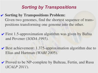
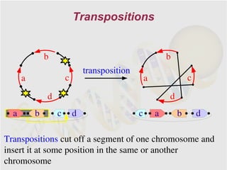
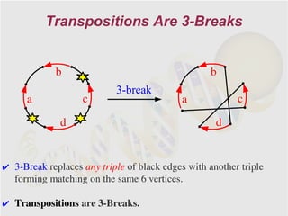
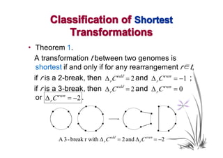
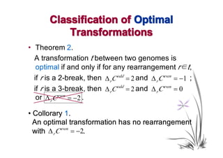
Download to read offline

![Previous Results
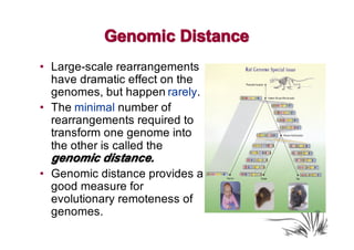
• The complexity of computing weighted genomic
distance remains unknown.
• Barder and Ohlebusch, 2007 developed a 1.5-
approximation algorithm for computing the weighted
genomic distance for α ∈ [1,2] .
• Eriksen, 2001 proposed a (1 + ε ) - approximation
algorithm for computing the weighted genomic
distance for α = 2, and any ε > 0.
• Blanchette et al, 1995, observed that if α ∈ (1,2), then
typical transformation still includes large proportion of
transpositions.](https://image.slidesharecdn.com/guests-2011-11-09-alekseyev-rearrangements-111120093308-phpapp01/85/Guests-2011-11-09-alekseyev-rearrangements-83-320.jpg)
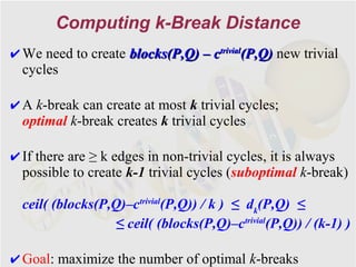
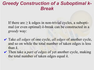
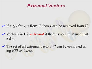
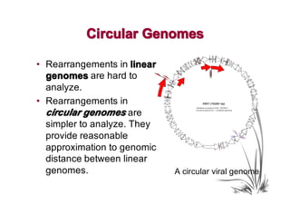
![Our Contribution
• We first characterize optimal transformations that at
transformations
the same time have the shortest length and make the
smallest number of cuts in the genomes, first introduced
by Alekseyev and Pevzner, PLoS Comput. Biol, 2007.
• Then, we prove that for α ∈ (1,2] , the weighted genomic
distance between two genomes with necessity
corresponds to an optimal tranformation between them.
• In particular, we show that a minimum-weight
transformation may entirely consist of transpositions.](https://image.slidesharecdn.com/guests-2011-11-09-alekseyev-rearrangements-111120093308-phpapp01/85/Guests-2011-11-09-alekseyev-rearrangements-84-320.jpg)
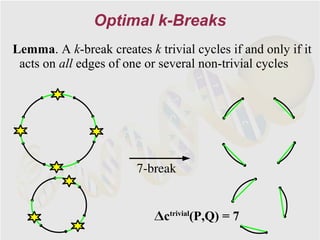
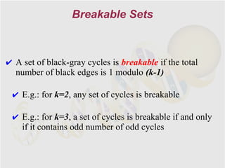
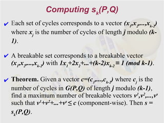
![Main Theorem
• Theorem 4.
For α ∈(1,2],
min {Wα ( t )} = Wα ( t 0 ),
t
where t goes over all transformations between
two genomes and t0 is any optimal
transformation between them.
• That is, for any α ∈(1,2], the weighted genomic
distance between two genomes equals the
weight of any optimal transformation between
them.](https://image.slidesharecdn.com/guests-2011-11-09-alekseyev-rearrangements-111120093308-phpapp01/85/Guests-2011-11-09-alekseyev-rearrangements-91-320.jpg)
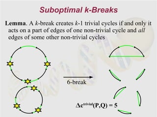
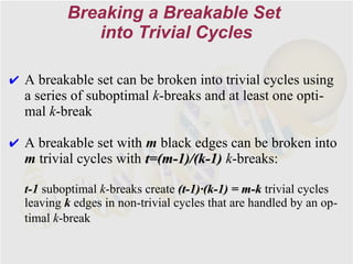
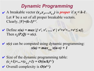
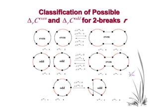
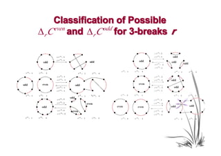
![Proof Idea
• We classify all possible changes in the numbers
of odd and even black-red cycles caused by a
rearrangement r.
• For an arbitrary transformation t and an optimal
transformation t0, we use our classification and
Theorem 4 to show that for any α ∈(1,2],
Wα (t ) ≥ Wα (t0 ).](https://image.slidesharecdn.com/guests-2011-11-09-alekseyev-rearrangements-111120093308-phpapp01/85/Guests-2011-11-09-alekseyev-rearrangements-92-320.jpg)
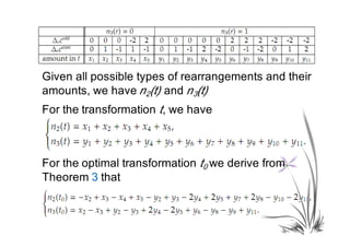
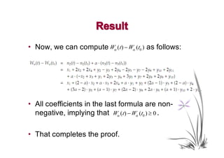
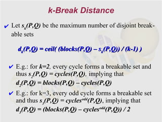
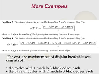
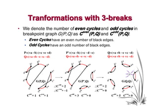
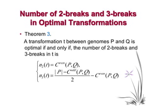
![Corollary
• For an optimal transformation t between
genomes P and Q, we have
� (Theorem 3)
⎧n2 (t ) = C even( P, Q),
⎪
⎨ | P | −C odd ( P, Q )
⎪n3 (t ) = − C even( P, Q)
⎩ 2
� (Theorem 4)
For any α ∈ (1,2], the weight of t equals the
weighted genomic distance between P and Q.
• Corollary 2.
If ∆C even (P, Q ) = 0, then transformationt has n2 (t ) = 0
and thus consists entirely 3-breaks (transpositions).](https://image.slidesharecdn.com/guests-2011-11-09-alekseyev-rearrangements-111120093308-phpapp01/85/Guests-2011-11-09-alekseyev-rearrangements-97-320.jpg)
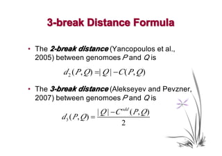
![Conclusions
• We proved that for α ∈(1,2] , the minimum-weight
transformations include the optimal
transformations that may entirely consist of
transposition-like rearrangements.
• Thus, the corresponding weighted genomic
distance does not actually impose any bound on
the proportion of transpositions.](https://image.slidesharecdn.com/guests-2011-11-09-alekseyev-rearrangements-111120093308-phpapp01/85/Guests-2011-11-09-alekseyev-rearrangements-98-320.jpg)

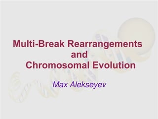
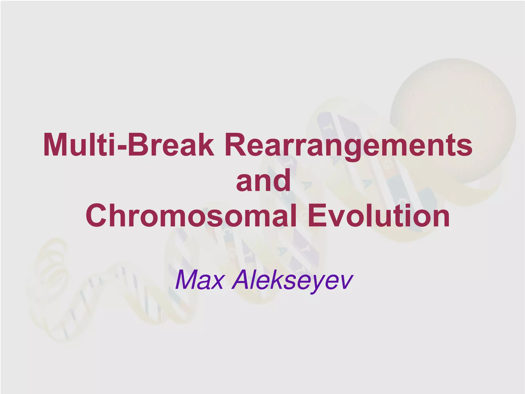
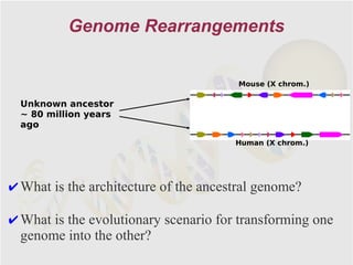
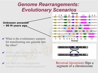
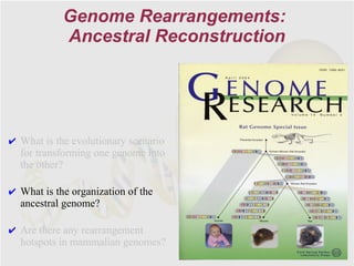
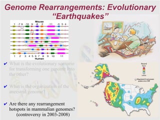
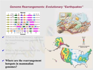
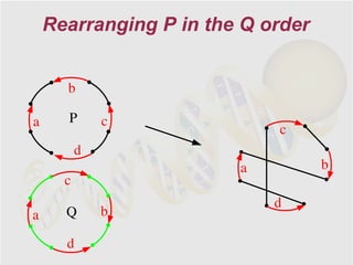
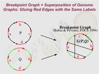
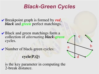
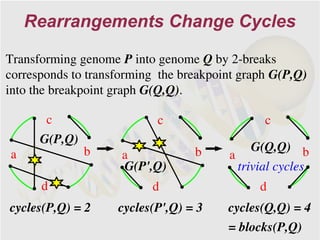
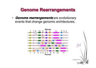
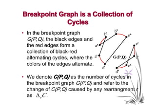
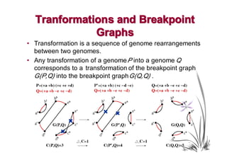
The document discusses genome rearrangements and chromosomal evolution. It begins by showing the X chromosomes of the mouse and human genomes and notes they diverged from an unknown common ancestor approximately 80 million years ago. It then poses questions about reconstructing the ancestral genome and the evolutionary scenario that transformed one genome into the other. The document goes on to discuss concepts like reversals, translocations, sorting genomes with rearrangements, and computing the rearrangement distance between genomes. It proposes modeling rearrangements as 2-break operations to more simply study rearrangements between multiple genomes.