Graph Matrices and Application, node reduction algorith
Graph Matrices and Application: Motivational overview, matrix of graph, relations, power of a matrix, node reduction algorithm, building tools. (Student should be given an exposure to a tool like JMeter or Win-runner).
Graph Matrices and Application, node reduction algorith
1.
Presented by
Dr. B.Rajalingam
AssociateProfessor
Department of Computer Science & Engineering
St. Martin's Engineering College
UNIT 5
Graph Matrices and Application
SOFTWARE TESTING METHODOLOGIES
2.
SOFTWARE TESTING METHODOLOGIES
Prerequisites
•1.A course on “Software Engineering”
Course Objectives
To provide knowledge of the concepts in software testing such as testing process, criteria,
strategies, and methodologies.
To develop skills in software test automation and management using latest tools.
Course Outcomes:
•Design and develop the best test strategies in accordance to the development model.
October 9, 2025 STM(Unit 5) : Dr. B.Rajalingam 2
3.
Syllabus
UNIT - I
Introduction:Purpose of testing, Dichotomies, model for testing, consequences of bugs,
taxonomy of bugs: Flow graphs and Path testing: Basics concepts of path testing, predicates, path
predicates and achievable paths, path sensitizing, path instrumentation, application of path testing.
UNIT - II
Transaction Flow Testing: transaction flows, transaction flow testing techniques. Dataflow
testing: Basics of dataflow testing, strategies in dataflow testing, application of dataflow testing. :
domains and paths, Nice & ugly domains, domain testing, domains and interfaces testing, domain
and interface testing, domains and testability.
October 9, 2025 STM(Unit 5) : Dr. B.Rajalingam 3
4.
Syllabus
UNIT - III
Paths,Path products and Regular expressions: path products & path expression, reduction procedure,
applications, regular expressions & flow anomaly detection.
Logic Based Testing: overview, decision tables, path expressions, kv charts, specifications.
UNIT - IV
State, State Graphs and Transition testing: state graphs, good & bad state graphs, state testing, Testability
tips.
UNIT - V
Graph Matrices and Application: Motivational overview, matrix of graph, relations, power of a matrix,
node reduction algorithm, building tools. (Student should be given an exposure to a tool like JMeter or
Win-runner).
October 9, 2025 STM(Unit 5) : Dr. B.Rajalingam 4
5.
TEXT BOOKS:
1. SoftwareTesting techniques – Baris Beizer, Dreamtech, second edition.
2. Software Testing Tools – Dr. K. V. K. K. Prasad, Dreamtech.
REFERENCE BOOKS:
1. The craft of software testing – Brian Marick, Pearson Education.
2. Software Testing Techniques – SPD(Oreille)
3. Software Testing in the Real World – Edward Kit, Pearson.
4. Effective methods of Software Testing, Perry, John Wiley.
5. Art of Software Testing – Meyers, John Wiley.
October 9, 2025 STM(Unit 5) : Dr. B.Rajalingam 5
6.
1. SYNOPSIS
• Graphmatrices are introduced as another representation for graphs
• Matrix operations
• Relations
• Node-reduction algorithm revisited
• Equivalence class partitions
October 9, 2025 STM(Unit 5) : Dr. B.Rajalingam 6
7.
2. MOTIVATIONAL OVERVIEW
2.1.The Problem with Pictorial Graphs
2.2. Tool Building
2.3. Doing and Understanding Testing Theory
2.4. The Basic Algorithms
October 9, 2025 STM(Unit 5) : Dr. B.Rajalingam 7
8.
2.1. The Problemwith Pictorial Graphs
• Whenever a graph is used as a model, sooner or later we trace paths through it—to find a set of
covering paths, a set of values that will sensitize paths, the logic function that controls the flow, the
processing time of the routine, the equations that define a domain, whether the routine pushes or
pops, or whether a state is reachable or not.
• Even algebraic representations such as BNF and regular expressions can be converted to equivalent
graphs.
• Much of test design consists of tracing paths through a graph and most testing strategies define some
kind of cover over some kind of graph.
• Path tracing is not easy, and it’s subject to error.
• You can miss a link here and there or cover some links twice—even if you do use a marking pen to
note which paths have been taken.
October 9, 2025 STM(Unit 5) : Dr. B.Rajalingam 8
9.
2.1. The Problemwith Pictorial Graphs
• You’re tracing a long complicated path through a routine when the telephone rings—you’ve lost your place
before you’ve had a chance to mark it.
• I get confused tracing paths, so naturally I assume that other people also get confused.
• One solution to this problem is to represent the graph as a matrix and to use matrix operations equivalent to path
tracing.
• These methods aren’t necessarily easier than path tracing, but because they’re more methodical and mechanical
and don’t depend on your ability to “see” a path, they’re more reliable.
• Even if you use powerful tools that do everything that can be done with graphs, and furthermore, enable you to
do it graphically, it’s still a good idea to know how to do it by hand; just as having a calculator should not mean
that you don’t need to know how to do arithmetic.
• Besides, with a little practice, you might find these methods easier and faster than doing it on the screen;
moreover, you can use them on the plane or anywhere.
October 9, 2025 STM(Unit 5) : Dr. B.Rajalingam 9
10.
2.2. Tool Building
•If you build test tools or want to know how they work, sooner or later you’ll be implementing or
investigating analysis routines based on these methods—or you should be.
• Think about how a naive tool builder would go about finding a property of all paths (a possibly
infinite number) versus how one might do it based on the methods.
• But it was graphical and it’s hard to build algorithms over visual graphs.
• The properties of graph matrices are fundamental to test tool building.
October 9, 2025 STM(Unit 5) : Dr. B.Rajalingam 10
11.
2.3. Doing andUnderstanding Testing Theory
• We talk about graphs in testing theory, but we prove theorems about graphs by proving
theorems about their matrix representations.
• Without the conceptual apparatus of graph matrices, you’ll be blind to much of testing theory,
especially those parts that lead to useful algorithms.
October 9, 2025 STM(Unit 5) : Dr. B.Rajalingam 11
12.
2.4. The BasicAlgorithms
• This is not intended to be a survey of graph-theoretic algorithms based on the matrix
representation of graphs.
• It’s intended only to be a basic toolkit.
• The basic toolkit consists of:
1. Matrix multiplication, which is used to get the path expression from every node to every other
node.
2. A partitioning algorithm for converting graphs with loops into loop-free graphs of equivalence
classes.
3. A collapsing process (analogous to the determinant of a matrix), which gets the path
expression from any node to any other node.
October 9, 2025 STM(Unit 5) : Dr. B.Rajalingam 12
13.
3. THE MATRIXOF A GRAPH
3.1. Basic Principles
3.2. A Simple Weight
3.3. Further Notation
October 9, 2025 STM(Unit 5) : Dr. B.Rajalingam 13
14.
3.1. Basic Principles
•A graph matrix is a square array with one row and one column for every node in the graph.
• Each row-column combination corresponds to a relation between the node corresponding to the
row and the node corresponding to the column.
• The relation, for example, could be as simple as the link name, if there is a link between the
nodes.
October 9, 2025 STM(Unit 5) : Dr. B.Rajalingam 14
15.
Examples of Graphsand their Associated Matrices
1. The size of the matrix (i.e., the number of rows and columns) equals the number of nodes.
2. There is a place to put every possible direct connection or link between any node and any other
node.
3. The entry at a row and column intersection is the link weight of the link (if any) that connects
the two nodes in that direction.
4. A connection from node i to node j does not imply a connection from node j to node i.
5. If there are several links between two nodes, then the entry is a sum; the “+” sign denotes
parallel links as usual.
October 9, 2025 STM(Unit 5) : Dr. B.Rajalingam 15
3.2. A SimpleWeight
• The simplest weight we can use is to note that there is or isn’t a connection.
• Let “1” mean that there is a connection and “0” that there isn’t.
• The arithmetic rules are:
• A matrix with weights defined like this is called a connection matrix.
• The connection matrix.1h is obtained by replacing each entry with I if there is a link and 0 if
there isn’t. As usual, to reduce clutter we don’t write down 0 entries.
• Each row of a matrix (whatever the weights) denotes the outlinks of the node corresponding to
that row, and each column denotes the inlinks corresponding to that node.
October 9, 2025 STM(Unit 5) : Dr. B.Rajalingam 17
1 + 1 = 1, 1 + 0 = 1, 0 + 0 = 0,
1 × 1 = 1, 1 × 0 = 0, 0 × 0 = 0.
18.
3.2. A SimpleWeight
• A branch node is a node with more than one nonzero entry in its row.
• A junction node is a node with more than one nonzero entry in its column.
• A self-loop is an entry along the diagonal.
• All have more than one entry, those nodes are branch nodes.
• Using the principle that a case statement is equivalent to n – 1 binary decisions, by subtracting 1
from the total number of entries in each row and ignoring rows with no entries (such as node 2),
we obtain the equivalent number of decisions for each row.
• Adding these values and then adding I to the sum yields the graph’s cyclomatic complexity.
October 9, 2025 STM(Unit 5) : Dr. B.Rajalingam 18
19.
3.3. Further Notation
October9, 2025 STM(Unit 5) : Dr. B.Rajalingam 19
• Talking about the “entry at row 6, column 7” is wordy.
• To compact things, the entry corresponding to node i and column j,
• which is to say the link weights between nodes i and j, is denoted by aij
.
• A self-loop about node i is denoted by aii
, while the link weight for the link between nodes j and
i is denoted by aji
.
• The path segments expressed in terms of link names and, in this notation, for several paths in
the graph of are:
20.
October 9, 2025STM(Unit 5) : Dr. B.Rajalingam 20
3.3. Further Notation
• The expression “aij
ajj
ajm
” denotes a path from node i
to j
, with a self-loop at j and then a link from node j to node
m.
• The expression “aij
ajk
akm
ami
” denotes a path from node i back to node i via nodes j, k, and m.
• An expression such as “aik
akm
amj
+ ain
anp
apj
” denotes a pair of paths between nodes i and j, one going via nodes k
and m and the other via nodes n and p.
• This notation may seem cumbersome, but it’s not intended for working with the matrix of a graph but for
expressing operations on the matrix. It’s a very compact notation.
• For example, denotes the set of all possible paths between nodes i and j via one intermediate node. But because “i”
and “j” denote any node, this expression is the set of all possible paths between any two nodes via one
intermediate node.
• The transpose of a matrix is the matrix with rows and columns interchanged.
• It is denoted by a superscript letter “T,” as in AT
. If C = AT
then cij
= aji
.
• The intersection of two matrices of the same size, denoted by A#B is a matrix obtained by an element-by-element
multiplication operation on the entries.
• For example, C = A#B means cij
= aij
#bij
.
• The multiplication operation is usually boolean AND or set intersection.
• Similarly, the union of two matrices is defined as the element-by-element addition operation such as a boolean OR
or set union.
21.
4. RELATIONS
4.1. General
•This isn’t a section on aunts and uncles but on abstract relations that can exist between abstract
objects, although family and personal relations can also be modeled by abstract relations, if you
want to.
• A relation is a property that exists between two (usually) objects of interest.
• Here’s a sample, where a and b denote objects and R is used to denote that a has the relation R
to b:
October 9, 2025 STM(Unit 5) : Dr. B.Rajalingam 21
22.
4. RELATIONS
October 9,2025 STM(Unit 5) : Dr. B.Rajalingam 22
1. “Node a is connected to node b” or aRb where “R” means “is connected to.”
2. “a >= b” or aRb where “R” means “greater than or equal.”
3. “a is a subset of b” where the relation is “is a subset of.”
4. “It takes 20 microseconds of processing time to get from node a to node b.” The relation is
expressed by the number 20.
5. “Data object X is defined at program node a and used at program node b.” The relation
between nodes a and b is that there is a du chain between them.
23.
Let’s now redefinewhat we mean by a graph.
• Graph consists of a set of abstract objects called nodes and a relation R between the nodes.
• If arb, which is to say that a has the relation R to b, it is denoted by a link from a to b. In
addition to the fact that the relation exists, for some relations we can associate one or more
properties.
• These are called link weights.
• A link weight can be numerical, logical, illogical, objective, subjective, or whatever.
• Furthermore, there is no limit to the number and type of link weights that one may associate
with a relation.
• “Is connected to” is just about the simplest relation there is: it is denoted by an unweighted link.
• Graphs defined over “is connected to” are called, as we said before, connection matrices.
• For more general relations, the matrix is called a relation matrix.
October 9, 2025 STM(Unit 5) : Dr. B.Rajalingam 23
24.
4.2. Properties ofRelations
4.2.1. General
4.2.2. Transitive Relations
4.2.3. Reflexive Relations
4.2.4. Symmetric Relations
4.2.5. Antisymmetric Relations
October 9, 2025 STM(Unit 5) : Dr. B.Rajalingam 24
25.
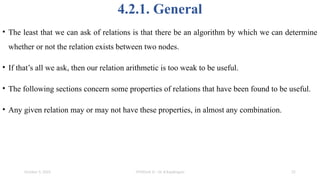
4.2.1. General
• Theleast that we can ask of relations is that there be an algorithm by which we can determine
whether or not the relation exists between two nodes.
• If that’s all we ask, then our relation arithmetic is too weak to be useful.
• The following sections concern some properties of relations that have been found to be useful.
• Any given relation may or may not have these properties, in almost any combination.
October 9, 2025 STM(Unit 5) : Dr. B.Rajalingam 25
26.
4.2.2. Transitive Relations
•A relation R is transitive if aRb and bRc implies aRc.
• Most relations used in testing are transitive.
• Examples of transitive relations include: is connected to, is greater than or equal to, is less than
or equal to, is a relative of, is faster than, is slower than, takes more time than, is a subset of,
includes, shadows, is the boss of.
• Examples of intransitive relations include: is acquainted with, is a friend of, is a neighbor of, is
lied to, has a du chain between.
October 9, 2025 STM(Unit 5) : Dr. B.Rajalingam 26
27.
4.2.3. Reflexive Relations
•A relation R is reflexive if, for every a, aRa. A reflexive relation is equivalent to a self-loop at
every node.
• Examples of reflexive relations include: equals, is acquainted with (except, perhaps, for
amnesiacs), is a relative of.
• Examples of irreflexive relations include: not equals, is a friend of (unfortunately), is on top of,
is under.
October 9, 2025 STM(Unit 5) : Dr. B.Rajalingam 27
28.
4.2.4. Symmetric Relations
October9, 2025 STM(Unit 5) : Dr. B.Rajalingam 28
• A relation R is symmetric if for every a and b, aRb implies bRa.
• A symmetric relation means that if there is a link from a to b then there is also a link from b to
a; which furthermore means that we can do away with arrows and replace the pair of links with
a single undirected link.
• A graph whose relations are not symmetric is called a directed graph because we must use
arrows to denote the relation’s direction.
• A graph over a symmetric relation is called an undirected graph.
• The matrix of an undirected graph is symmetric (aij
= aji
for all i, j)
29.
4.2.5. Antisymmetric Relations
•A relation R is antisymmetric if for every a and b, if aRb and bRa, then a = b, or they are the
same elements.
• Examples of antisymmetric relations: is greater than or equal to, is a subset of, time.
• Examples of nonantisymmetric relations: is connected to, can be reached from, is greater than,
is a relative of, is a friend of.
October 9, 2025 STM(Unit 5) : Dr. B.Rajalingam 29
30.
4.3. Equivalence Relations
•An equivalence relation is a relation that satisfies the reflexive, transitive, and symmetric
properties.
• Numerical equality is the most familiar example of an equivalence relation.
• If a set of objects satisfy an equivalence relation, we say that they form an equivalence class
over that relation.
• The importance of equivalence classes and relations is that any member of the equivalence class
is, with respect to the relation, equivalent to any other member of that class.
• The idea behind partition-testing strategies such as domain testing and path testing, is that we
can partition the input space into equivalence classes.
October 9, 2025 STM(Unit 5) : Dr. B.Rajalingam 30
31.
4.3. Equivalence Relations
•The idea behind partition-testing strategies such as domain testing and path testing, is that we
can partition the input space into equivalence classes.
• If we can do that, then testing any member of the equivalence class is as effective as testing
them all.
• When we say in path testing that it is sufficient to test one set of input values for each member
of a branch-covering set of paths, we are asserting that the set of all input values for each path
(e.g., the path’s domain) is an equivalence class with respect to the relation that defines branch-
testing paths.
• If we furthermore (incorrectly) assert that a strategy such as branch testing is sufficient, we are
asserting that satisfying the branch-testing relation implies that all other possible equivalence
relations will also be satisfied—that, of course, is nonsense.
October 9, 2025 STM(Unit 5) : Dr. B.Rajalingam 31
32.
4.4. Partial OrderingRelations
• A partial ordering relation satisfies the reflexive, transitive, and antisymmetric properties.
• Partial ordered graphs have several important properties: they are loop-free, there is at least one
maximum element, there is at least one minimum element, and if you reverse all the arrows, the
resulting graph is also partly ordered.
• A maximum element a is one for which the relation xRa does not hold for any other element x.
Similarly, a minimum element a, is one for which the relation aRx does not hold for any other
element x. Trees are good examples of partial ordering.
• The importance of partial ordering is that while strict ordering (as for numbers) is rare with
graphs, partial ordering is common.
October 9, 2025 STM(Unit 5) : Dr. B.Rajalingam 32
33.
4.4. Partial OrderingRelations
• The importance of partial ordering is that while strict ordering (as for numbers) is rare with
graphs, partial ordering is common. Loop-free graphs are partly ordered.
• We have many examples of useful partly ordered graphs: call trees, most data structures, an
integration plan.
• Also, whereas the general control-flow or data-flow graph is not always partly ordered, we’ve
seen that by restricting our attention to partly ordered graphs we can sometimes get new, useful
strategies.
• Also, it is often possible to remove the loops from a graph that isn’t partly ordered to obtain
another graph that is.
October 9, 2025 STM(Unit 5) : Dr. B.Rajalingam 33
34.
5. THE POWERSOF A MATRIX
5.1. Principles
5.2. Matrix Powers and Products
5.3. The Set of All Paths
5.4. Loops
5.5. Partitioning Algorithm (BEIZ71, SOHO84)
5.6. Breaking Loops And Applications
October 9, 2025 STM(Unit 5) : Dr. B.Rajalingam 34
35.
5.1. Principles
• Eachentry in the graph’s matrix (that is, each link) expresses a relation between the pair of nodes that
corresponds to that entry.
• It is a direct relation, but we are usually interested in indirect relations that exist by virtue of intervening
nodes between the two nodes of interest.
• Squaring the matrix (using suitable arithmetic for the weights) yields a new matrix that expresses the
relation between each pair of nodes via one intermediate node under the assumption that the relation is
transitive.
• The square of the matrix represents all path segments two links long.
• Similarly, the third power represents all path segments three links long.
• And the kth power of the matrix represents all path segments k links long.
• Because a matrix has at most n nodes, and no path can be more than n – 1 links long without
incorporating some path segment already accounted for, it is generally not necessary to go beyond the n
– 1 power of the matrix.
• As usual, concatenation of links or the weights of links is represented by multiplication, and parallel
links or path expressions by addition.
October 9, 2025 STM(Unit 5) : Dr. B.Rajalingam 35
36.
5.1. Principles
October 9,2025 STM(Unit 5) : Dr. B.Rajalingam 36
• Let A be a matrix whose entries are aij
.
• The set of all paths between any node i and any other node j (possibly i itself), via all possible
intermediate nodes, is given by
• As formidable as this expression might appear, it states nothing more than the following:
1. Consider the relation between every node and its neighbor.
2. Extend that relation by considering each neighbor as an intermediate node.
3. Extend further by considering each neighbor’s neighbor as an intermediate node.
4. Continue until the longest possible nonrepeating path has been established.
5. Do this for every pair of nodes in the graph.
37.
5.2. Matrix Powersand Products
October 9, 2025 STM(Unit 5) : Dr. B.Rajalingam 37
• Given a matrix whose entries are aij
, the square of that matrix is obtained by replacing every
entry with
• More generally, given two matrices A and B, with entries aik
and bkj
, respectively, their product
is a new matrix C, whose entries are cij
, where:
38.
5.2. Matrix Powersand Products
October 9, 2025 STM(Unit 5) : Dr. B.Rajalingam 38
• The indexes of the product [e.g., (3,2) in C32
] identify, respectively, the row of the first matrix
and the column of the second matrix that will be combined to yield the entry for that product in
the product matrix.
• The C32
entry is obtained by combining, element by element, the entries in the third row of the
A matrix with the corresponding elements in the second column of the B matrix.
• I use two hands.
• My left hand points and traces across the row while the right points down the column of B.
• It’s like patting your head with one hand and rubbing your stomach with the other at the same
time: it takes practice to get the hang of it.
39.
5.2. Matrix Powersand Products
October 9, 2025 STM(Unit 5) : Dr. B.Rajalingam 39
• A2
A = AA2
; that is, matrix multiplication is associative (for most interesting relations) if the
underlying relation arithmetic is associative.
• Therefore, you can get A4
in any of the following ways: A2
A2
, (A2
)2
, A3
A, AA3
.
• However, because multiplication is not necessarily commutative, you must remember to put the
contribution of the left-hand matrix in front of the contribution of the right-hand matrix and not
inadvertently reverse the order.
• The loop terms are important.
• These are the terms that appear along the principal diagonal (the one that slants down to the
right).
• The initial matrix had a self-loop about node 5, link h.
• No new loop is revealed with paths of length 2, but the cube of the matrix shows additional
loops about nodes 3 (bfe), 4 (feb), and 5 (ebf).
• It’s clear that these are the same loop around the three nodes.
40.
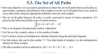
5.3. The Setof All Paths
• Our main objective is to use matrix operations to obtain the set of all paths between all nodes or,
equivalently, a property (described by link weights) over the set of all paths from every node to
every other node, using the appropriate arithmetic rules for such weights.
• The set of all paths between all nodes is easily expressed in terms of matrix operations. It’s
given by the following infinite series of matrix powers:
• This is an eloquent, but practically useless, expression.
• Let I be an n by n matrix, where n is the number of nodes.
• Let I’s entries consist of multiplicative identity elements along the principal diagonal.
• For link names, this can be the number “1.” For other kinds of weights, it is the multiplicative
identity for those weights.
• The above product can be re-phrased as: A(I + A + A2
+ A3
+ A4
. . . A∞
)
October 9, 2025 STM(Unit 5) : Dr. B.Rajalingam 40
41.
5.3. The Setof All Paths
• But often for relations, A + A = A, (A + I)2
= A2
+ A +A + I A2
+ A + I. Furthermore, for any
finite n,
(A + I)n
= I + A + A2
+ A3
. . . An
• Therefore, the original infinite sum can be replaced by
• This is an improvement, because in the original expression we had both infinite products and
infinite sums, and now we have only one infinite product to contend with.
• The above is valid whether or not there are loops. If we restrict our interest for the moment to
paths of length n – 1, where n is the number of nodes, the set of all such paths is given by
• This is an interesting set of paths because, with n nodes, no path can exceed n – 1 nodes without
incorporating some path segment that is already incorporated in some other path or path
segment.
• Finding the set of all such paths is somewhat easier because it is not necessary to do all the
intermediate products explicitly.
October 9, 2025 STM(Unit 5) : Dr. B.Rajalingam 41
42.
5.3. The Setof All Paths
October 9, 2025 STM(Unit 5) : Dr. B.Rajalingam 42
The following algorithm is effective:
1. Express n – 2 as a binary number.
2. Take successive squares of (A + I), leading to (A + I)2
, (A + I)4
, (A + 1)8
, and so on.
3. Keep only those binary powers of (A + 1) that correspond to a 1 value in the binary
representation of n – 2.
4. The set of all paths of length n – 1 or less is obtained as the product of the matrices you got
in step 3 with the original matrix.
43.
5.3. The Setof All Paths
October 9, 2025 STM(Unit 5) : Dr. B.Rajalingam 43
• The binary representation of n – 2 (14) is 23
+ 22
+ 2. Consequently, the set of paths is given by
• This required one multiplication to get the square, squaring that to get the fourth power, and
squaring again to get the eighth power, then three more multiplications to get the sum, for a
total of six matrix multiplications without additions, compared to fourteen multiplications and
additions if gotten directly.
• A matrix for which A2
= A is said to be idempotent.
• A matrix whose successive powers eventually yields an idempotent matrix is called an
idempotent generator—that is, a matrix for which there is a k
such that Ak+1
= Ak
.
• The point about idempotent generator matrices is that we can get properties over all paths by
successive squaring. A graph matrix of the form (A + I) over a transitive relation is an
idempotent generator; therefore, anything of interest can be obtained by even simpler means
than the binary method discussed above.
• For example, the relation “connected” does not change once we reach An-1
because no
connection can take more than n – 1 links and, once connected, nodes cannot be disconnected.
44.
5.3. The Setof All Paths
October 9, 2025 STM(Unit 5) : Dr. B.Rajalingam 44
• Thus, if we wanted to know which nodes of an n-node graph were connected to which, by
whatever paths, we have only to calculate: A2
, A2
A2
= A4
. . . AP
, where p is the next power of 2
greater than or equal to n.
• We can do this because the relation “is connected to” is reflexive and transitive.
• The fact that it is reflexive means that every node has the equivalent of a self-loop, and the
matrix is therefore an idempotent generator.
• If a relation is transitive but not reflexive, we can augment it as we did above, by adding the
unit matrix to it, thereby making it reflexive.
• That is, although the relation defined over A is not reflexive, A + I is. A + I is an idempotent
generator, and therefore there’s nothing new to learn for powers greater than n – 1, the length of
the longest nonrepeating path through the graph.
• The nth power of a matrix A + I over a transitive relation is called the transitive closure of the
matrix.
45.
5.4. Loops
October 9,2025 STM(Unit 5) : Dr. B.Rajalingam 45
• Every loop forces us into a potentially infinite sum of matrix powers.
• The way to handle loops is similar to what we did for regular expressions.
• Every loop shows up as a term in the diagonal of some power of the matrix—the power at which the
loop finally closes—or, equivalently, the length of the loop.
• The impact of the loop can be obtained by preceding every element in the row of the node at which the
loop occurs by the path expression of the loop term starred and then deleting the loop term.
• Applying this method of characterizing all possible paths is straightforward.
• The above operations are interpreted in terms of the arithmetic appropriate to the weights used.
• Note, however, that if you are working with predicates and you want the logical function (predicate
function, truth-value function) between every node and every other node, this may lead to loops in the
logical functions.
• Code that leads to predicate loops is not very nice, not well structured, hard to understand, and harder to
test—and anyone who codes that way deserves the analytical difficulties arising therefrom.
• Predicate loops come about from declared or undeclared program switches and/or unstructured loop
constructs.
• This means that the routine’s code remembers.
• If you didn’t realize that you put such a loop in, you probably didn’t intend to.
• If you did intend it, you should have expected the loop.
46.
5.5. Partitioning Algorithm(BEIZ71, SOHO84)
October 9, 2025 STM(Unit 5) : Dr. B.Rajalingam 46
• Consider any graph over a transitive relation.
• The graph may have loops.
• We would like to partition the graph by grouping nodes in such a way that every loop is
contained within one group or another. Such a graph is partly ordered.
• There are many used for an algorithm that does that:
1. We might want to embed the loops within a subroutine so as to have a resulting graph
which is loop-free at the top level.
2. Many graphs with loops are easy to analyze if you know where to break the loops.
3. While you and I can recognize loops, it’s much harder to program a tool to do it unless you
have a solid algorithm on which to base the tool.
• The way to do this is straightforward.
• Calculate the following matrix: (A + I)n
# (A + I)nT
.
• This groups the nodes into strongly connected sets of nodes such that the sets are partly ordered.
47.
5.5. Partitioning Algorithm(BEIZ71, SOHO84)
October 9, 2025 STM(Unit 5) : Dr. B.Rajalingam 47
• Furthermore, every such set is an equivalence class so that any one node in it represents the set.
• Now consider all the places in this book where we said “except for graphs with loops” or
“assume a loop-free graph” or words to that effect.
• If you can bury the loop in a real subroutine, you can as easily bury it in a conceptual
subroutine.
• Do the analysis over the partly ordered graph obtained by the partitioning algorithm and treat
each loop-connected node set as if it is a subroutine to be examined in detail later.
• For each such component, break the loop and repeat the process. You now have a divide-and-
conquer approach for handling loops. Here’s an example, worked with an arbitrary graph:
48.
Here’s an example,worked with an arbitrary graph:
October 9, 2025 STM(Unit 5) : Dr. B.Rajalingam 48
The relation matrix is The transitive closure matrix is Intersection with its
transpose yields
Arbitrary graph
• You can recognize equivalent nodes by simply picking a row (or column) and searching the matrix for identical
rows.
• Mark the nodes that match the pattern as you go and eliminate that row.
• Then start again from the top with another row and another pattern.
• Eventually, all rows have been grouped.
• The algorithm leads to the following equivalent node sets:
A = [1], B = [2,7] , C = [3,4,5], D = [6] , E = [8]
whose graph is
49.
5.6. Breaking Loopsand Applications
October 9, 2025 STM(Unit 5) : Dr. B.Rajalingam 49
• Consider the matrix of a strongly connected subgraph.
• If there are entries on the principal diagonal, then start by breaking the loop for those links.
• At some power or another, a loop is manifested as an entry on the principal diagonal.
• Furthermore, the regular expression over the link names that appears in the diagonal entry tells
you all the places you can or must break the loop.
• Another way is to apply the node-reduction algorithm, which will also display the loops and
therefore the desired break points.
• The divide-and-conquer, or rather partition-and-conquer, properties of the equivalence
partitioning algorithm is a basis for implementing tools.
• The problem with most algorithms is that they are computationally intensive and require of the
order of n2
or n3
arithmetic operations, where n is the number of nodes.
• Even with fast, cheap computers it’s hard to keep up with such growth laws.
• The key to solving big problems (hundreds of nodes) is to partition them into a hierarchy of
smaller problems.
• If you can go far enough, you can achieve processing of the order of n, which is fine.
• The partition algorithm makes graphs into trees, which are relatively easy to handle.
50.
6. NODE-REDUCTION ALGORITHM
October9, 2025 STM(Unit 5) : Dr. B.Rajalingam 50
6.1. General
6.2. Some Matrix Properties
6.3. The Algorithm
6.4. Applications
6.5. Some Hints
51.
6.1. General
October 9,2025 STM(Unit 5) : Dr. B.Rajalingam 51
• The matrix powers usually tell us more than we want to know about most graphs.
• In the context of testing, we’re usually interested in establishing a relation between two nodes
— typically the entry and exit nodes—rather than between every node and every other node.
• In a debugging context it is unlikely that we would want to know the path expression between
every node and every other node; there also, it is the path expression or some other related
expression between a specific pair of nodes that is sought: for example,
• The advantage of the matrix-reduction method is that it is more methodical than the graphical
method and does not entail continually redrawing the graph.
52.
Cont…
October 9, 2025STM(Unit 5) : Dr. B.Rajalingam 52
1. Select a node for removal; replace the node by equivalent links that bypass that
node and add those links to the links they parallel.
2. Combine the parallel terms and simplify as you can.
3. Observe loop terms and adjust the outlinks of every node that had a self-loop to
account for the effect of the loop.
4. The result is a matrix whose size has been reduced by 1. Continue until only the
two nodes of interest exist.
53.
October 9, 2025STM(Unit 5) : Dr. B.Rajalingam 53
6.2. Some Matrix Properties
• If you numbered the nodes of a graph from 1 to n, you would not expect that the
behavior of the graph or the program that it represents would change if you happened to
number the nodes differently.
• Node numbering is arbitrary and cannot affect anything.
• The equivalent to renumbering the nodes of a graph is to interchange the rows and
columns of the corresponding matrix.
• Say that you wanted to change the names of nodes i and j to j and i, respectively.
• You would do this on the graph by erasing the names and rewriting them.
• To interchange node names in the matrix, you must interchange both the corresponding
rows and the corresponding columns.
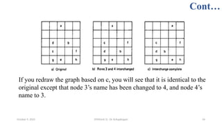
• Interchanging the names of nodes 3 and 4 in the graph of Figure results in the following:
54.
Cont…
October 9, 2025STM(Unit 5) : Dr. B.Rajalingam 54
If you redraw the graph based on c, you will see that it is identical to the
original except that node 3’s name has been changed to 4, and node 4’s
name to 3.
55.
6.3. The Algorithm
October9, 2025 STM(Unit 5) : Dr. B.Rajalingam 55
• The first step is the most complicated one:
• eliminating a node and replacing it with a set of equivalent links.
• Using the example of Figure, we must first remove the self-loop at node 5. This
produces the following matrix:
56.
Cont…
October 9, 2025STM(Unit 5) : Dr. B.Rajalingam 56
• The reduction is done one node at a time by combining the elements in the last column with the
elements in the last row and putting the result into the entry at the corresponding intersection.
• In the above case, the f in column 5 is first combined with h*g in column 2, and the result (fh*g)
is added to the c term just above it.
• Similarly, the f is combined with h*e in column 3 and put into the 4,3 entry just above it.
• The justification for this operation is that the column entry specifies the links entering the node,
whereas the row specifies the links leaving the node.
• Combining every column entry with the corresponding row entries for that node produces
exactly the same result as the node-elimination step in the graphical-reduction procedure.
• What we did was: a45
a52
= a42
or f × h*g = a52
, but because there was already a c term there, we
have effectively created a parallel link in the (5,2) position leading to the complete term of c +
fh*g.
• The matrix resulting from this step is
57.
Cont…
October 9, 2025STM(Unit 5) : Dr. B.Rajalingam 57
• If any loop terms had occurred at this point, they would have been
taken care of by eliminating the loop term and premultiplying every
term in that row by the loop term starred.
• There are no loop terms at this point.
• The next node to be removed is node 4.
• The b term in the (3,4) position will combine with the (4,2) and (4,3)
terms to yield a (3,2) and a (3,3) term, respectively.
• Carrying this out and discarding the unnecessary rows and columns
yields
58.
Cont…
October 9, 2025STM(Unit 5) : Dr. B.Rajalingam 58
Removing the loop term yields
There is only one node to remove now, node 3.
This will result in a term in the (1,2) entry whose value is
a(bfh*e)*(d + bc + bfh*g)
59.
Cont…
October 9, 2025STM(Unit 5) : Dr. B.Rajalingam 59
• This is the path expression from node 1 to
node 2.
• Stare at this one for awhile before you
object to the (bfh*e)* term that multiplies
the d; any fool can see the direct path via d
from node 1 to the exit, but you could miss
the fact that the routine could circulate
around nodes 3, 4, and 5 before it finally
took the d link to node 2.
60.
6.4. Applications
October 9,2025 STM(Unit 5) : Dr. B.Rajalingam 60
6.4.1. General
6.4.2. Maximum Number of Paths
6.4.3. The Probability of Getting There
6.4.4. Get/Return Problem
6.5. Some Hints
61.
6.4.1. General
October 9,2025 STM(Unit 5) : Dr. B.Rajalingam 61
• The path expression is usually the most difficult and complicated to get.
• The arithmetic rules for most applications are simpler.
• In this section we’ll redo applications from, using the appropriate arithmetic rules,
but this time using matrices rather than graphs.
62.
6.4.2. Maximum Numberof Paths
October 9, 2025 STM(Unit 5) : Dr. B.Rajalingam 62
• The matrix corresponding to the graph on page 261 is on the opposite page.
• The successive steps are shown.
• Recall that the inner loop about nodes 8 and 9 was to be taken from zero to three times, while
the outer loop about nodes 5 and 10 was to be taken exactly four times.
• This will affect the way the diagonal loop terms are handled.
63.
6.4.3. The Probabilityof Getting There
October 9, 2025 STM(Unit 5) : Dr. B.Rajalingam 63
• A matrix representation for the probability problem on page 268 is
64.
6.4.4. Get/Return Problem
•The GET/RETURN problem on page 276 has the following matrix reduction:
October 9, 2025 STM(Unit 5) : Dr. B.Rajalingam 64
65.
6.5. Some Hints
•Redrawing the matrix over and over again is as bad as redrawing the graph to which it
corresponds.
• You actually do the work in place.
• Things get more complicated, and expressions get bigger as you progress, so you make the low-
numbered boxes larger than the boxes corresponding to higher-numbered nodes, because those
are the ones that are going to be removed first.
• Mark the diagonal lightly so that you can easily see the loops.
• With these points in mind, the work sheet for the timing analysis graph on page 272 looks like
this:
October 9, 2025 STM(Unit 5) : Dr. B.Rajalingam 65
66.
7. BUILDING TOOLS
October9, 2025 STM(Unit 5) : Dr. B.Rajalingam 66
7.1. Matrix Representation Software
7.1.1. Overview
7.1.2. Node Degree and Graph Density
7.1.3. What’s Wrong with Arrays?
7.1.4. Linked-List Representation
7.2. Matrix Operations
7.2.1. Parallel Reduction
7.2.2. Loop Reduction
7.2.3. Cross-Term Reduction
7.2.4 Addition, Multiplication, and Other Operations
7.3. Node-Reduction Optimization
67.
7.1. Matrix RepresentationSoftware
October 9, 2025 STM(Unit 5) : Dr. B.Rajalingam 67
7.1.1. Overview
7.1.2. Node Degree and Graph Density
68.
7.1.1. Overview
October 9,2025 STM(Unit 5) : Dr. B.Rajalingam 68
• We draw graphs or display them on screens as visual objects;
• we prove theorems and develop graph algorithms by using matrices;
• and when we want to process graphs in a computer, because we’re building tools, we represent
them as linked lists.
• We use linked lists because graph matrices are usually very sparse; that is, the rows and
columns are mostly empty.
69.
7.1.2. Node Degreeand Graph Density
October 9, 2025 STM(Unit 5) : Dr. B.Rajalingam 69
• The out-degree of a node is the number of outlinks it has.
• The in-degree of a node is the number of inlinks it has.
• The degree of a node is the sum of the out-degree and in-degree.
• The average degree of a node (the mean over all nodes) for a typical graph defined over
software is between 3 and 4.
• The degree of a simple branch is 3, as is the degree of a simple junction.
• The degree of a loop, if wholly contained in one statement, is only 4.
• A mean node degree of 5 or 6 say, would be a very busy flowgraph indeed.
70.
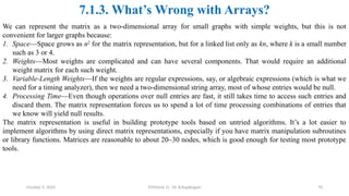
7.1.3. What’s Wrongwith Arrays?
October 9, 2025 STM(Unit 5) : Dr. B.Rajalingam 70
We can represent the matrix as a two-dimensional array for small graphs with simple weights, but this is not
convenient for larger graphs because:
1. Space—Space grows as n2
for the matrix representation, but for a linked list only as kn, where k is a small number
such as 3 or 4.
2. Weights—Most weights are complicated and can have several components. That would require an additional
weight matrix for each such weight.
3. Variable-Length Weights—If the weights are regular expressions, say, or algebraic expressions (which is what we
need for a timing analyzer), then we need a two-dimensional string array, most of whose entries would be null.
4. Processing Time—Even though operations over null entries are fast, it still takes time to access such entries and
discard them. The matrix representation forces us to spend a lot of time processing combinations of entries that
we know will yield null results.
The matrix representation is useful in building prototype tools based on untried algorithms. It’s a lot easier to
implement algorithms by using direct matrix representations, especially if you have matrix manipulation subroutines
or library functions. Matrices are reasonable to about 20–30 nodes, which is good enough for testing most prototype
tools.
71.
7.1.4. Linked-List Representation
October9, 2025 STM(Unit 5) : Dr. B.Rajalingam 71
• Give every node a unique name or number.
• A link is a pair of node names.
• Note that I’ve put the list entries in lexicographic order.
• The link names will usually be pointers to entries in a string array Where the actual link weight
expressions are stored.
• If the weights are fixed length then they can be associated directly with the links in a parallel, fixed
entry-length array.
• Let’s clarify the notation a bit by using node names and pointers.
72.
Cont…
October 9, 2025STM(Unit 5) : Dr. B.Rajalingam 72
• The node names appear only once, at the first link entry. Also, instead of naming the other end of the link, we have just the pointer to the list
position in which that node starts. Finally, it is also very useful to have back pointers for the in links. Doing this we get
• It’s important to keep the lists sorted in lexicographic ordering with the following priorities: node names or pointers, outlink names or pointers,
inlink names or pointers.
• Because the various operations will result in nearly sorted lists, a sort algorithm, such as string sort, that’s optimum for such lists is an essential
subroutine.
73.
7.2. Matrix Operations
October9, 2025 STM(Unit 5) : Dr. B.Rajalingam 73
7.2.1. Parallel Reduction
7.2.2. Loop Reduction
7.2.3. Cross-Term Reduction
7.2.4 Addition, Multiplication, and Other Operations
74.
7.2.1. Parallel Reduction
October9, 2025 STM(Unit 5) : Dr. B.Rajalingam 74
This is the easiest operation. Parallel links after sorting are adjacent entries with the same pair of
node names. For example:
We have three parallel links from node 17 to node 44.
We fetch the weight expressions using the y, z, and w pointers and we obtain a new link that is their sum:
75.
7.2.2. Loop Reduction
October9, 2025 STM(Unit 5) : Dr. B.Rajalingam 75
• Loop reduction is almost as easy.
• A loop term is spotted as a self-link.
• The effect of the loop must be applied to all the outlinks of the node.
• Scan the link list for the node to find the loop(s).
• Apply the loop calculation to every outlink, except another loop.
• Remove that loop. Repeat for all loops about that node. Repeat for all nodes.
For example removing node 5’s loop:
List Entry
76.
7.2.3. Cross-Term Reduction
October9, 2025 STM(Unit 5) : Dr. B.Rajalingam 76
• Select a node for reduction.
• The cross-term step requires that you combine every inlink to the node with every outlink from that node.
• The outlinks are associated with the node you’ve selected.
• The inlinks are obtained by using the back pointers.
• The new links created by removing the node will be associated with the nodes of the inlinks.
• Say that the node to be removed was node 4.
• As implemented, you can remove several nodes in one pass if you do careful bookkeeping and keep your pointers straight.
• The links created by node removal are stored in a separate list which is then sorted and thereafter merged into the master list.
77.
7.2.4 Addition, Multiplication,and Other Operations
October 9, 2025 STM(Unit 5) : Dr. B.Rajalingam 77
• Addition of two matrices is straightforward.
• If you keep the lists sorted, then simply merge the lists and combine parallel entries.
• Multiplication is more complicated but also straightforward.
• You have to beat the node’s outlinks against the list’s inlinks.
• It can be done in place, but it’s easier to create a new list.
• Again, the list will be in sorted order and you use parallel combination to do the addition and to
compact the list.
• Transposition is done by reversing the pointer directions, resulting in a list that is not correctly
sorted.
• Sorting that list provides the transpose.
• All other matrix operations can be easily implemented by sorting, merging, and combining
parallels.
78.
7.3. Node-Reduction Optimization
October9, 2025 STM(Unit 5) : Dr. B.Rajalingam 78
• The optimum order for node reduction is to do lowest-degree nodes first.
• The idea is to get the lists as short as possible as quickly as possible.
• Nodes of degree 3 (one in and two out or two in and one out) reduce the total link count by one link
when removed.
• A degree-4 node keeps the link count the same, and all higher-degree nodes increase the link count.
• Although this is not guaranteed, by picking the lowest-degree node available for reduction you can
almost prevent unlimited list growth.
• Because processing is dominated by list length rather than by the number of nodes on the list, this
strategy is effective.
• For large graphs with 500 or more nodes and an average degree of 6 or 7, the difference between not
optimizing the node-reduction order and optimizing it was about 50: 1 in processing time.
79.
8. Summary
October 9,2025 STM(Unit 5) : Dr. B.Rajalingam 79
1. Working with pictorial graphs is tedious and a waste of time. Graph matrices are used to organize the work.
2. The graph matrix is the tool of choice for proving things about graphs and for developing algorithms.
3. As implemented in tools, graph matrices are usually represented as linked lists.
4. Most testing problems can be recast into an equivalent problem about some graph whose links have one or more
weights and for which there is a problem—specific arithmetic over the link weights. The link-weighted graph is
represented by a relation matrix.
5. Relations as abstract operators are well understood and have interesting properties which can be exploited to
create efficient algorithms. Properties of interest include transitivity, reflexivity, symmetry, asymmetry, and
antisymmetry. These properties in various combinations define ordering, partial ordering, and equivalence
relations.
6. The powers of a relation matrix define relations spanning one, two, three, and up to the maximum number of links
that can be included in a path. The powers of the matrix are the primary tool for finding properties that relate any
node to any other node.
7. The transitive closure of the matrix is used to define equivalence classes and to convert an arbitrary graph into a
partly ordered graph.
8. The node reduction algorithm first presented in Chapter is redefined in terms of matrix operations.
9. There is an old and copious literature on graph matrices and associated algorithms. Serious tool builders should
learn that literature lest they waste time reinventing ancient algorithms or on marginally useful heuristics.


![5.2. Matrix Powers and Products
October 9, 2025 STM(Unit 5) : Dr. B.Rajalingam 38
• The indexes of the product [e.g., (3,2) in C32
] identify, respectively, the row of the first matrix
and the column of the second matrix that will be combined to yield the entry for that product in
the product matrix.
• The C32
entry is obtained by combining, element by element, the entries in the third row of the
A matrix with the corresponding elements in the second column of the B matrix.
• I use two hands.
• My left hand points and traces across the row while the right points down the column of B.
• It’s like patting your head with one hand and rubbing your stomach with the other at the same
time: it takes practice to get the hang of it.](https://image.slidesharecdn.com/stmunit5-251009233551-84d12575/85/Graph-Matrices-and-Application-node-reduction-algorith-38-320.jpg)


![Here’s an example, worked with an arbitrary graph:
October 9, 2025 STM(Unit 5) : Dr. B.Rajalingam 48
The relation matrix is The transitive closure matrix is Intersection with its
transpose yields
Arbitrary graph
• You can recognize equivalent nodes by simply picking a row (or column) and searching the matrix for identical
rows.
• Mark the nodes that match the pattern as you go and eliminate that row.
• Then start again from the top with another row and another pattern.
• Eventually, all rows have been grouped.
• The algorithm leads to the following equivalent node sets:
A = [1], B = [2,7] , C = [3,4,5], D = [6] , E = [8]
whose graph is](https://image.slidesharecdn.com/stmunit5-251009233551-84d12575/85/Graph-Matrices-and-Application-node-reduction-algorith-48-320.jpg)