lecture for description open channel flow as non uniform gradually varied flow in open channels

1. Gradually varied flow
Arturo S. Leon, PhD, PE, D.WRE

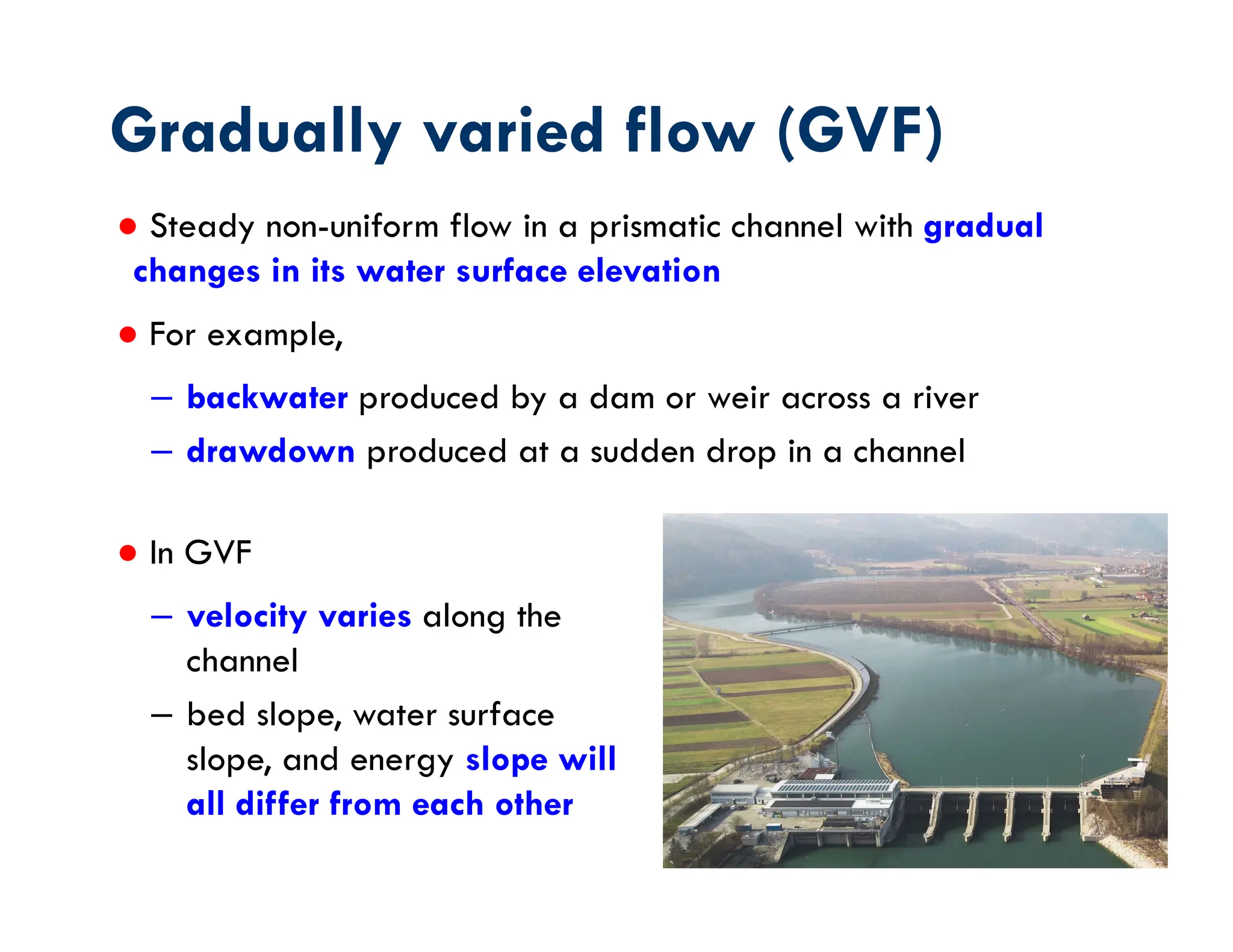
2. ● Steady non-uniform flow in a prismatic channel with gradual
changes in its water surface elevation
● For example,
– backwater produced by a dam or weir across a river
– drawdown produced at a sudden drop in a channel
Gradually varied flow (GVF)
● In GVF
– velocity varies along the
channel
– bed slope, water surface
slope, and energy slope will
all differ from each other

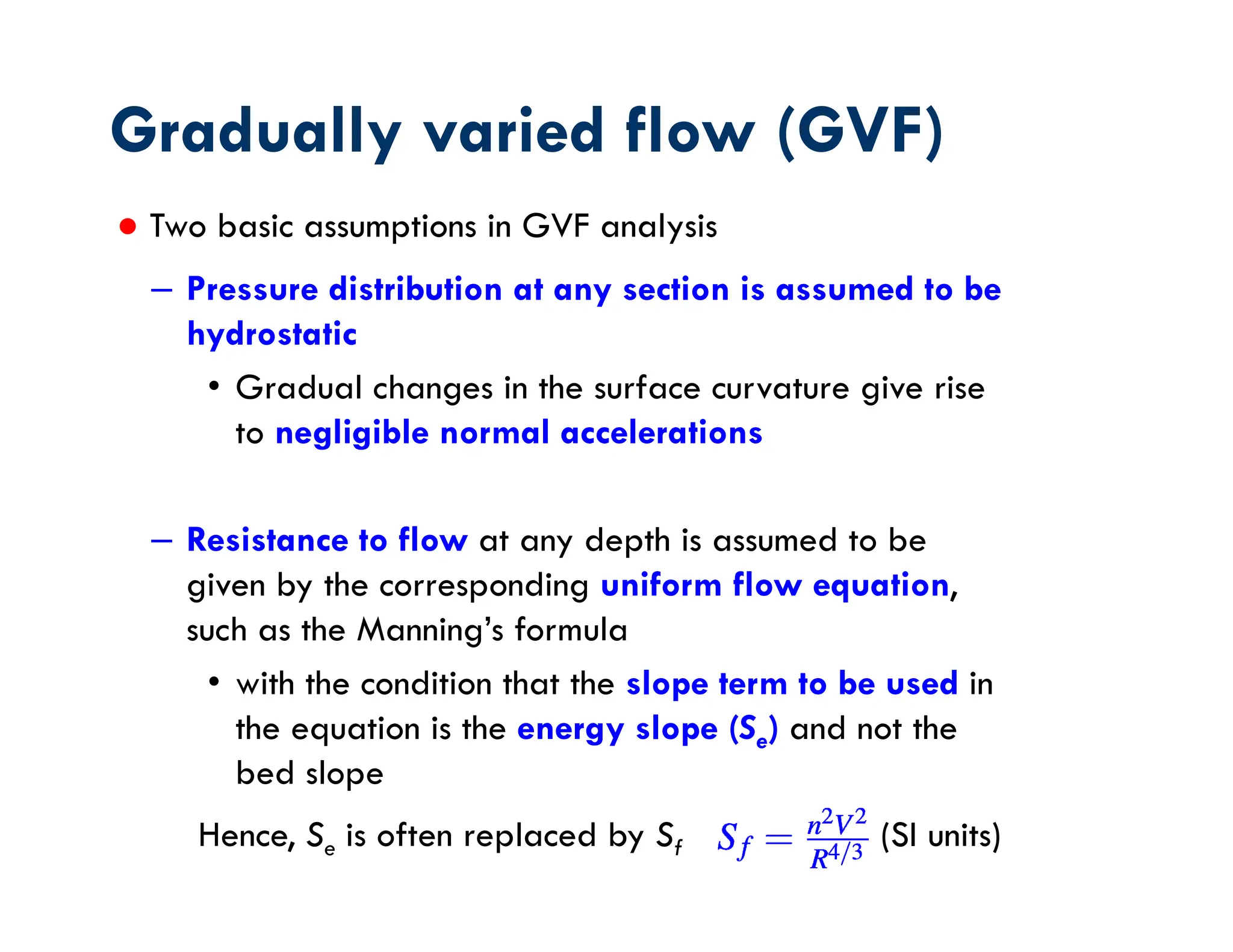
3. ● Two basic assumptions in GVF analysis
– Pressure distribution at any section is assumed to be
hydrostatic
• Gradual changes in the surface curvature give rise
to negligible normal accelerations
– Resistance to flow at any depth is assumed to be
given by the corresponding uniform flow equation,
such as the Manning’s formula
• with the condition that the slope term to be used in
the equation is the energy slope (Se) and not the
bed slope
Gradually varied flow (GVF)
Hence, Se is often replaced by Sf (SI units)

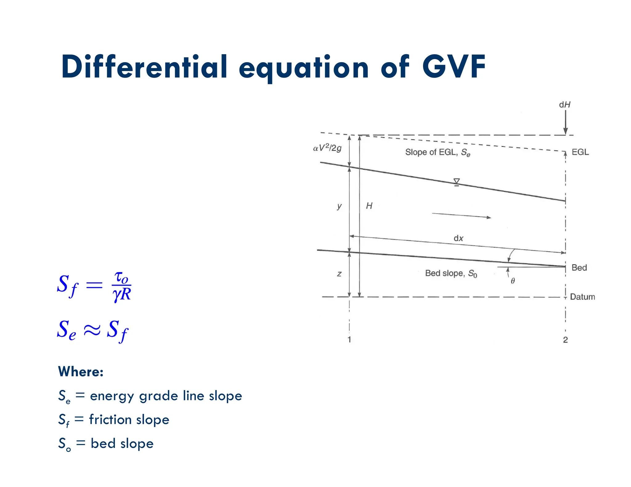
4. Where:
Se = energy grade line slope
Sf = friction slope
So = bed slope
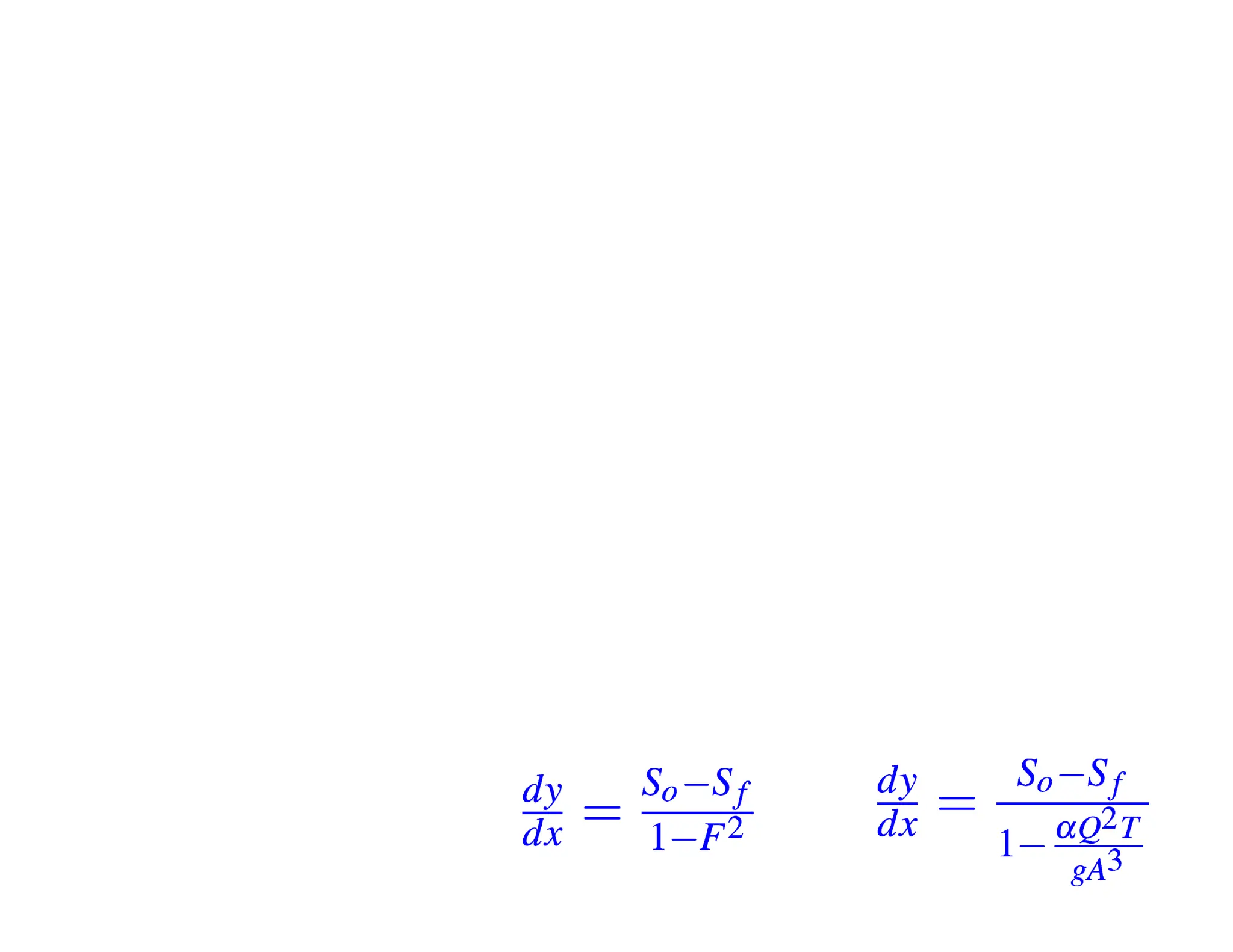
Differential equation of GVF

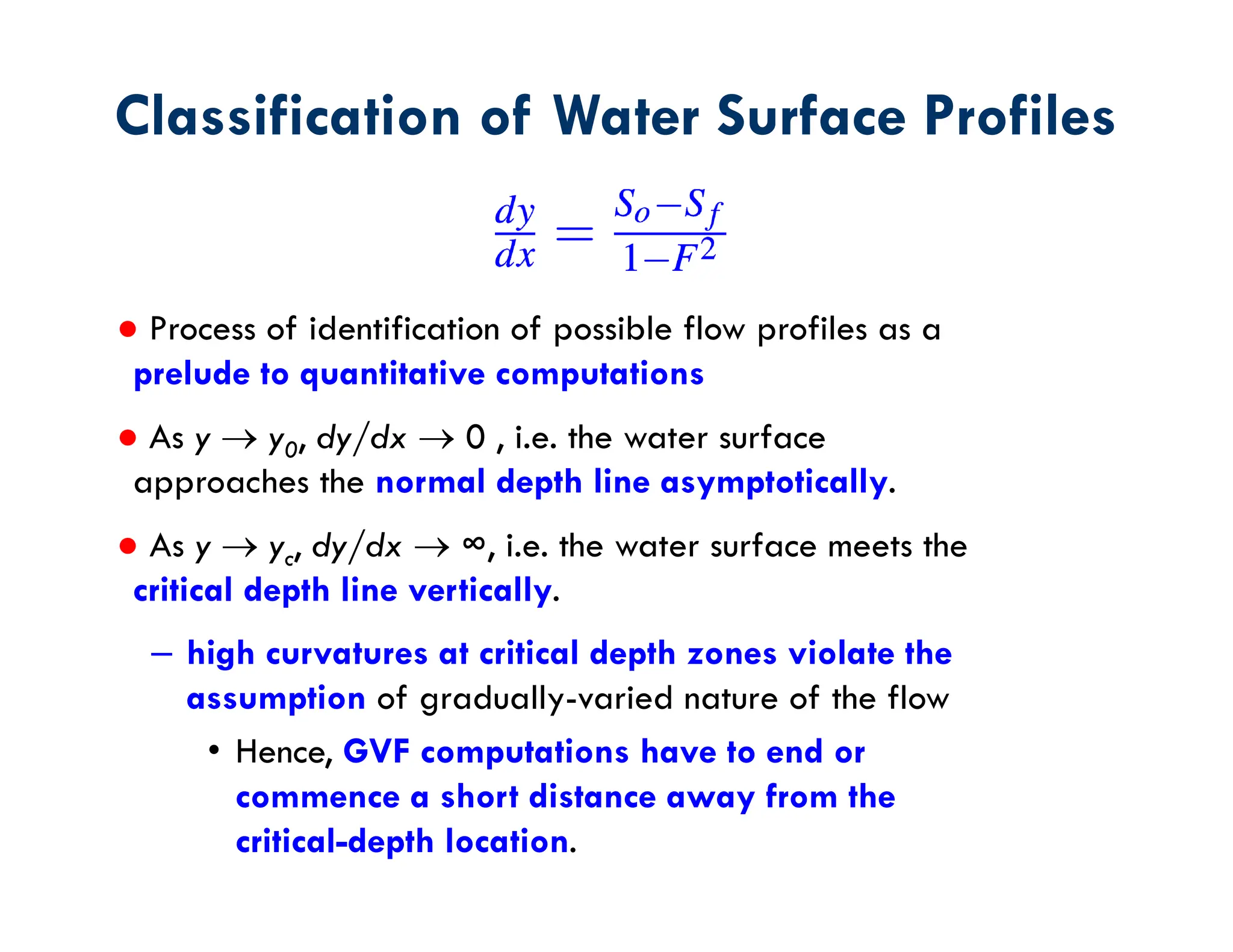
7. ● Process of identification of possible flow profiles as a
prelude to quantitative computations
● As y  y0, dy/dx  0 , i.e. the water surface
approaches the normal depth line asymptotically.
● As y  yc, dy/dx  ∞, i.e. the water surface meets the
critical depth line vertically.
– high curvatures at critical depth zones violate the
assumption of gradually-varied nature of the flow
• Hence, GVF computations have to end or
commence a short distance away from the
critical-depth location.
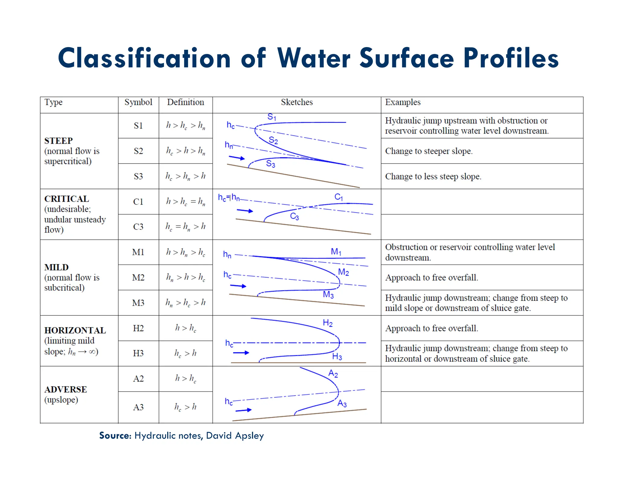
Classification of Water Surface Profiles

8. Source: Hydraulic notes, David Apsley
Classification of Water Surface Profiles

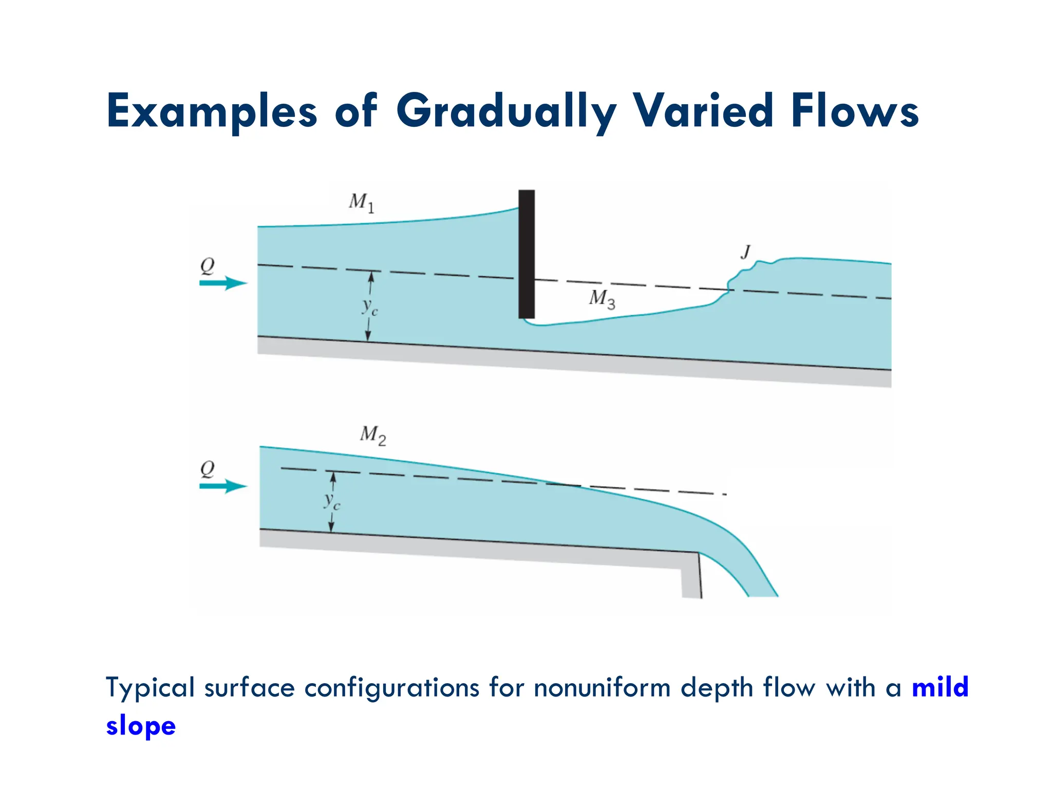
9. Examples of Gradually Varied Flows
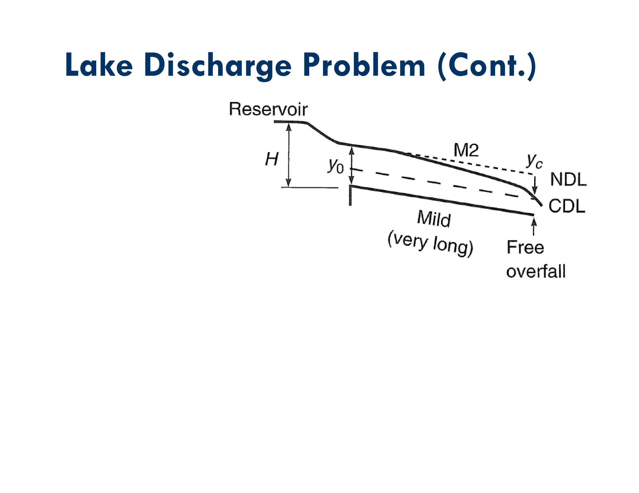
Typical surface configurations for nonuniform depth flow with a mild
slope

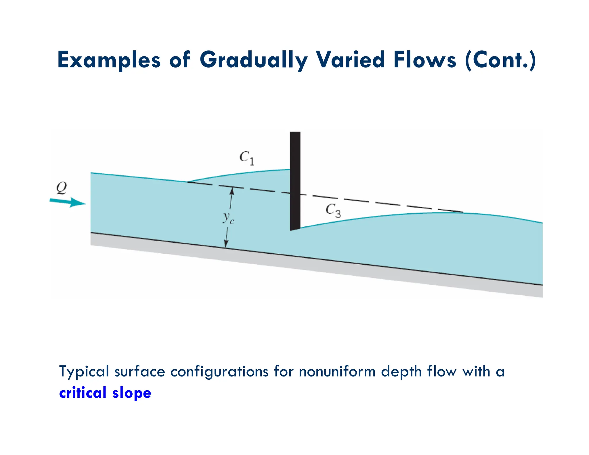
10. Examples of Gradually Varied Flows (Cont.)
Typical surface configurations for nonuniform depth flow with a
critical slope

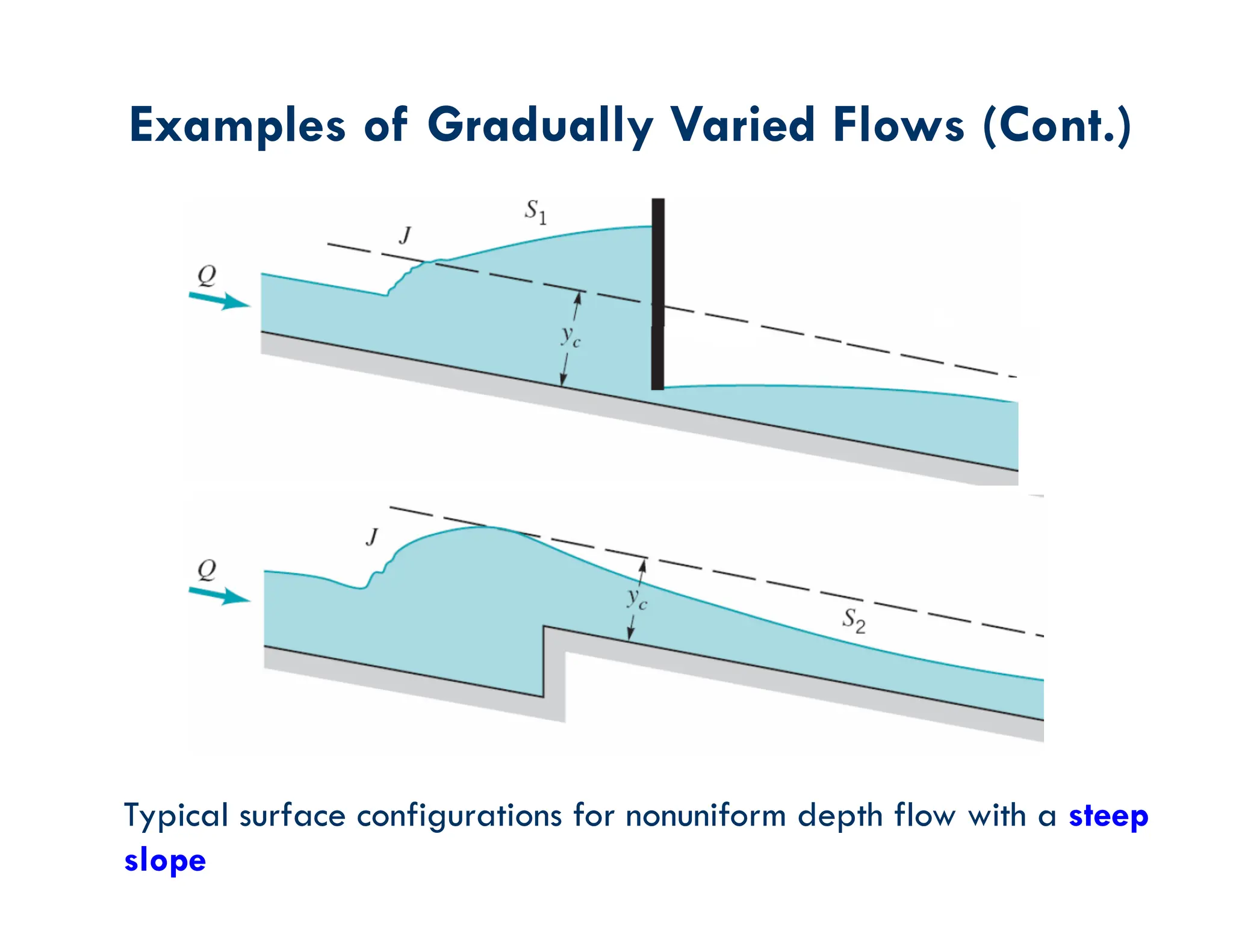
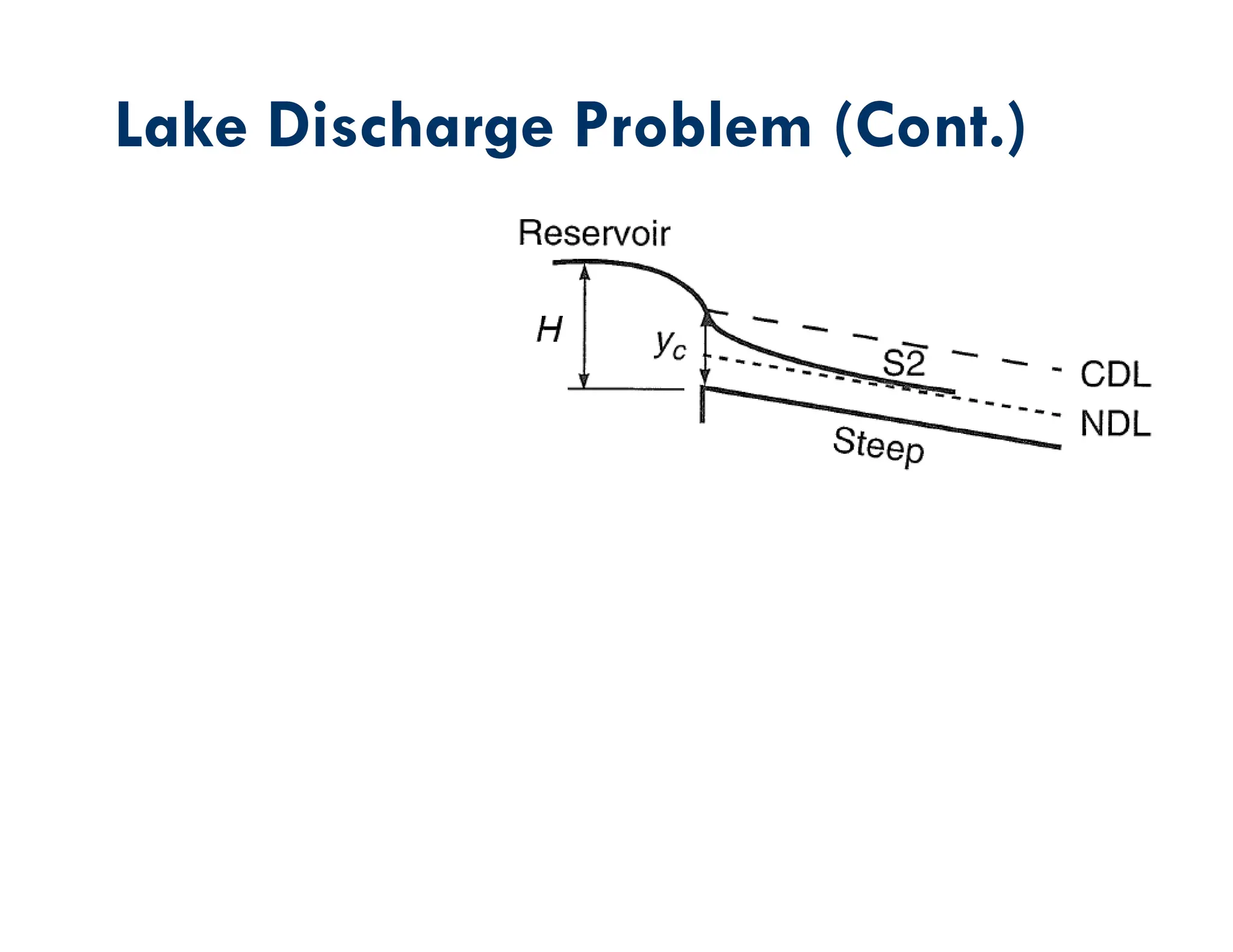
11. Examples of Gradually Varied Flows (Cont.)
Typical surface configurations for nonuniform depth flow with a steep
slope

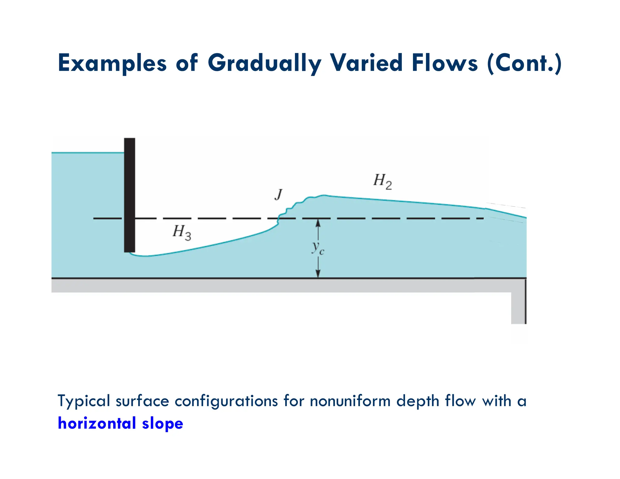
12. Examples of Gradually Varied Flows (Cont.)
Typical surface configurations for nonuniform depth flow with a
horizontal slope

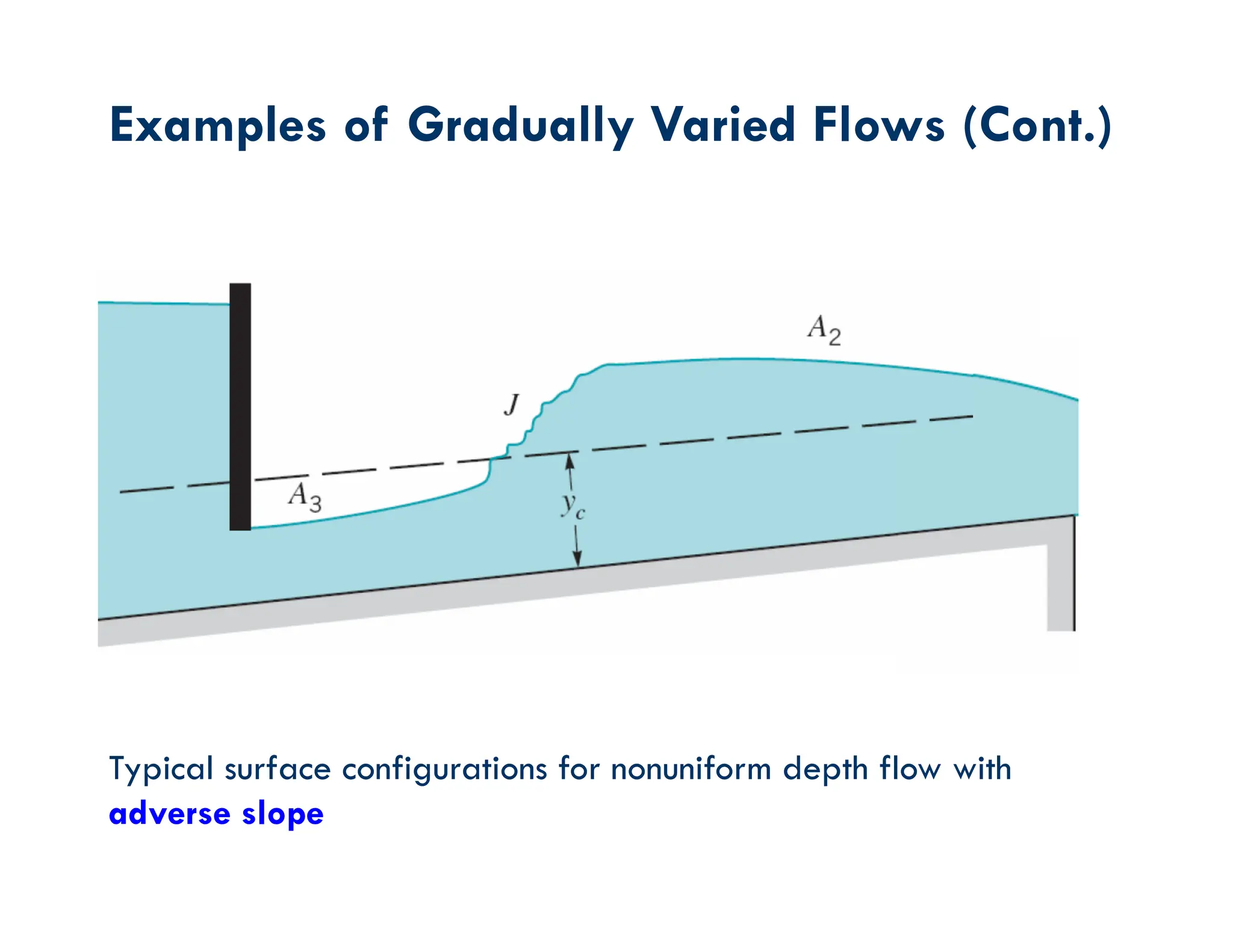
13. Examples of Gradually Varied Flows (Cont.)
Typical surface configurations for nonuniform depth flow with
adverse slope

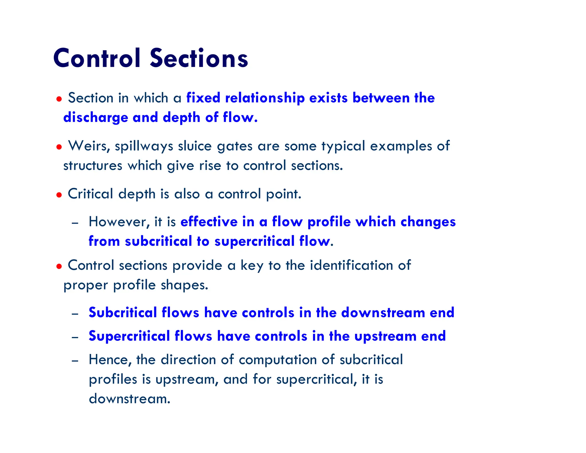
14. Control Sections
● Section in which a fixed relationship exists between the
discharge and depth of flow.
● Weirs, spillways sluice gates are some typical examples of
structures which give rise to control sections.
● Critical depth is also a control point.
– However, it is effective in a flow profile which changes
from subcritical to supercritical flow.
● Control sections provide a key to the identification of
proper profile shapes.
– Subcritical flows have controls in the downstream end
– Supercritical flows have controls in the upstream end
– Hence, the direction of computation of subcritical
profiles is upstream, and for supercritical, it is
downstream.

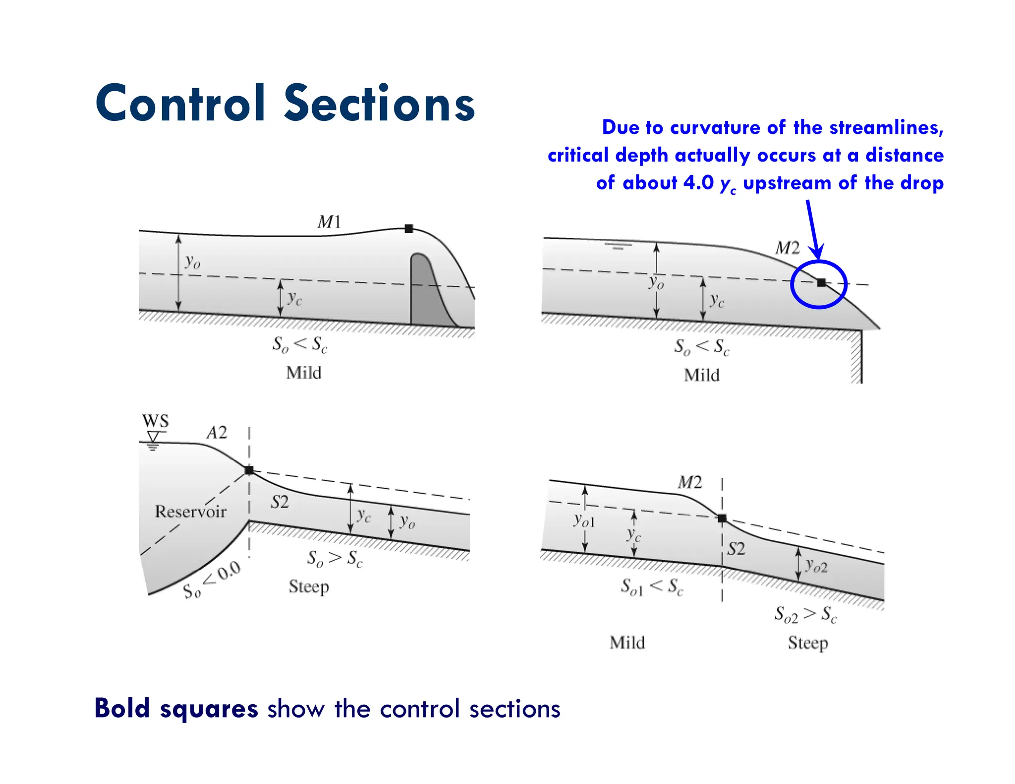
15. Control Sections
Bold squares show the control sections
Due to curvature of the streamlines,
critical depth actually occurs at a distance
of about 4.0 yc upstream of the drop

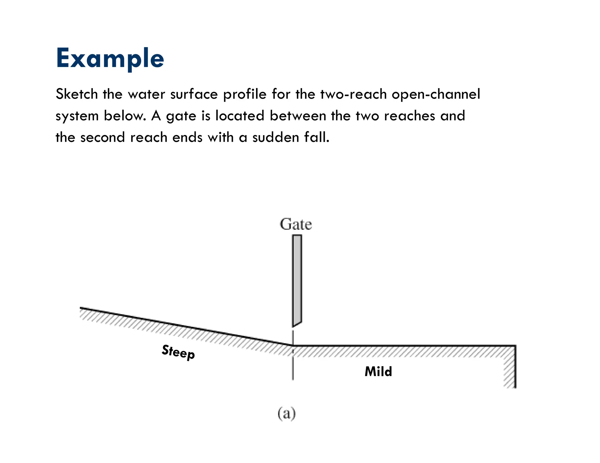
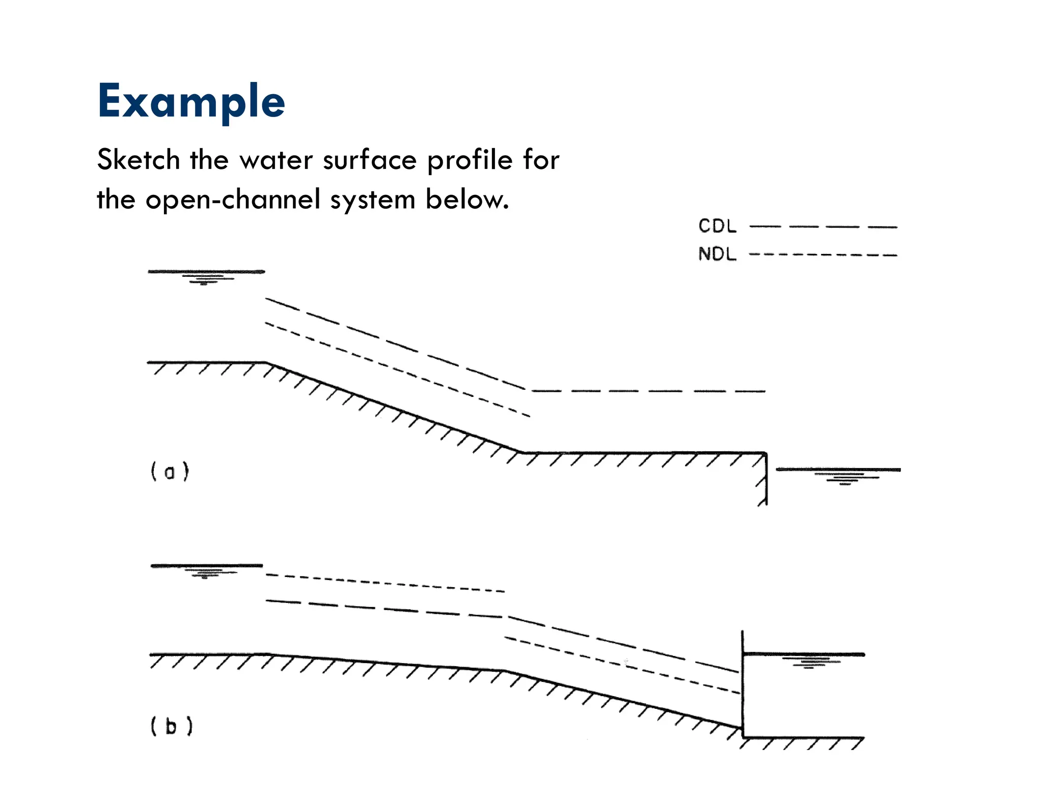
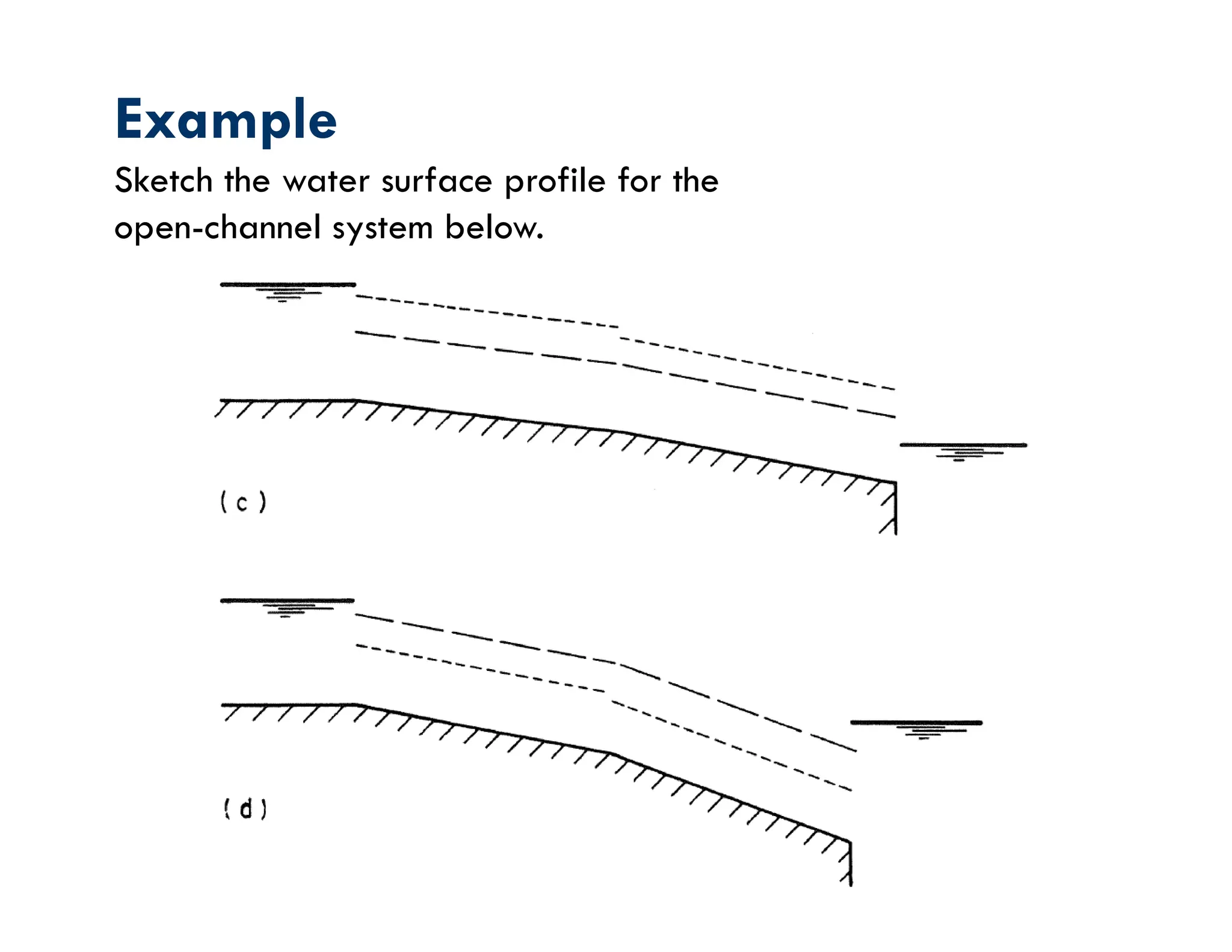
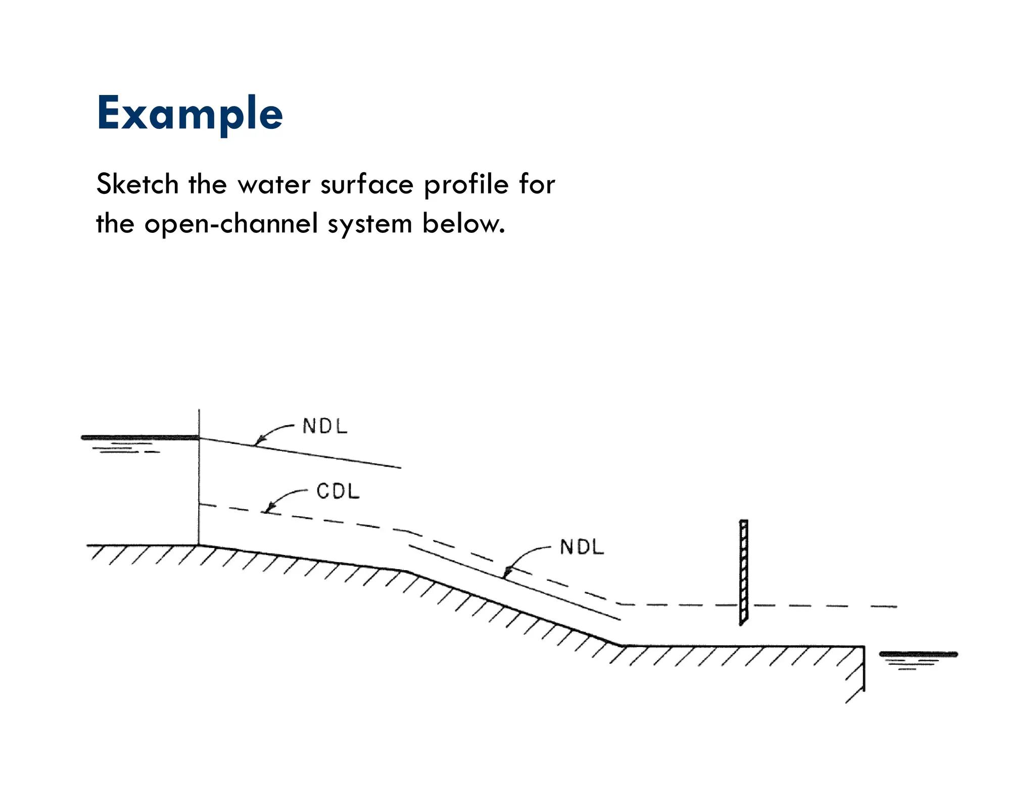
16. Example
Sketch the water surface profile for the two-reach open-channel
system below. A gate is located between the two reaches and
the second reach ends with a sudden fall.
Mild

17. Example
Sketch the water surface profile for the
open-channel system below.
Reservoir
Reservoir

18. Example
Sketch the water surface profile for
the open-channel system below.

19. Example
Sketch the water surface profile for the
open-channel system below.

20. Example
Sketch the water surface profile for
the open-channel system below.

21. Lake Discharge
Problem
Difficult to know discharge,
because it is unclear whether
slope is mild or steep

22. Lake Discharge Problem (Cont.)

23. Lake Discharge Problem (Cont.)

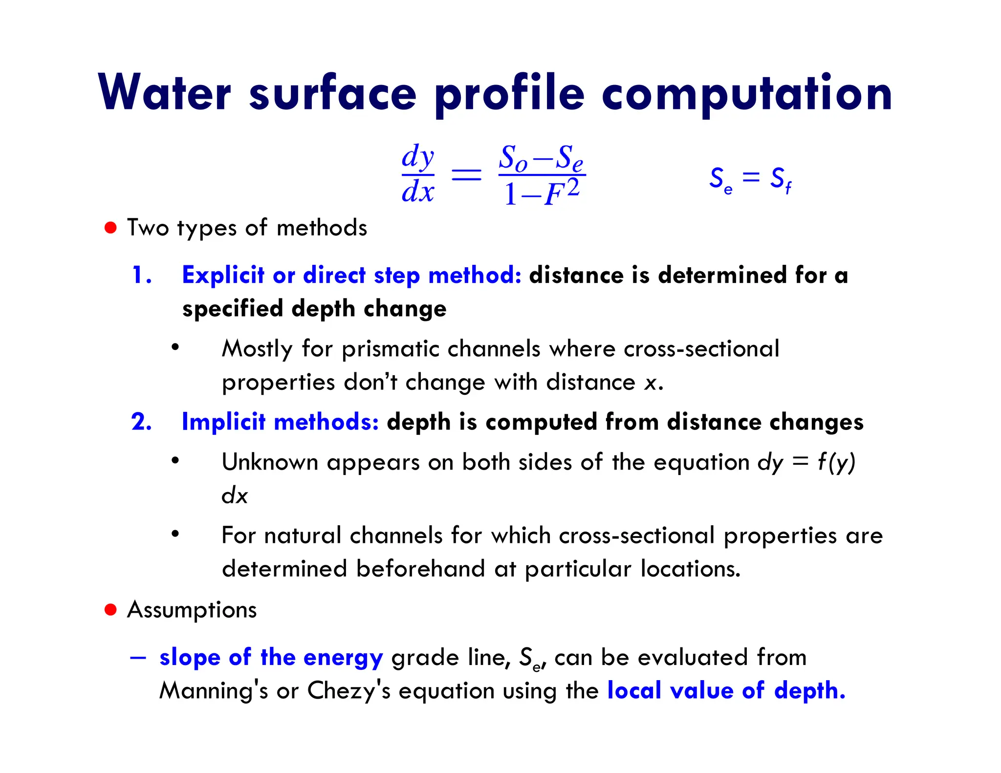
24. Water surface profile computation
● Two types of methods
1. Explicit or direct step method: distance is determined for a
specified depth change
• Mostly for prismatic channels where cross-sectional
properties don’t change with distance x.
2. Implicit methods: depth is computed from distance changes
• Unknown appears on both sides of the equation dy = f(y)
dx
• For natural channels for which cross-sectional properties are
determined beforehand at particular locations.
● Assumptions
– slope of the energy grade line, Se, can be evaluated from
Manning's or Chezy's equation using the local value of depth.
Se = Sf

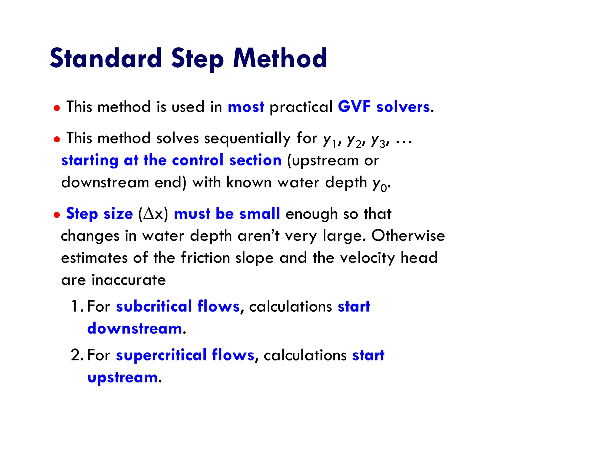
25. Standard Step Method
● This method is used in most practical GVF solvers.
● This method solves sequentially for y1, y2, y3, …
starting at the control section (upstream or
downstream end) with known water depth y0.
● Step size (x) must be small enough so that
changes in water depth aren’t very large. Otherwise
estimates of the friction slope and the velocity head
are inaccurate
1. For subcritical flows, calculations start
downstream.
2. For supercritical flows, calculations start
upstream.

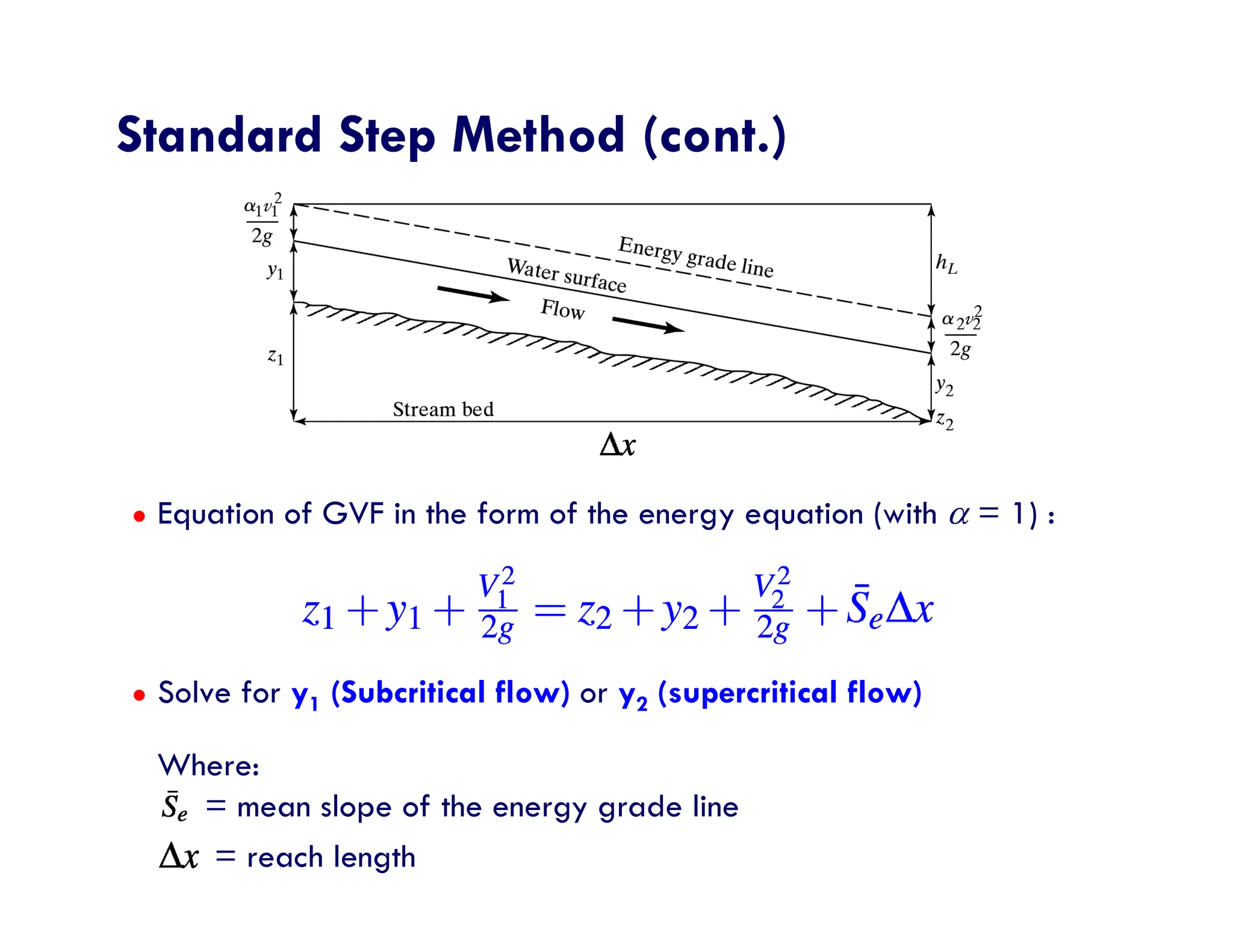
26. Standard Step Method (cont.)
● Equation of GVF in the form of the energy equation (with  = 1) :
● Solve for y1 (Subcritical flow) or y2 (supercritical flow)
Where:
= mean slope of the energy grade line
= reach length

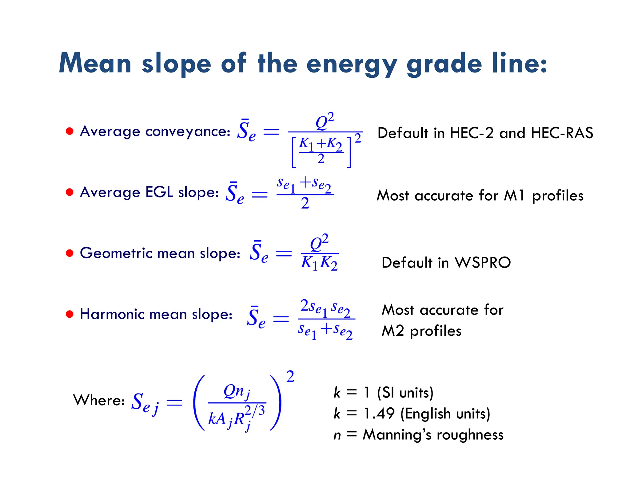
27. Mean slope of the energy grade line:
Default in HEC-2 and HEC-RAS
Default in WSPRO
Most accurate for M1 profiles
Most accurate for
M2 profiles
● Average conveyance:
● Average EGL slope:
● Geometric mean slope:
● Harmonic mean slope:
Where: k = 1 (SI units)
k = 1.49 (English units)
n = Manning’s roughness

28. Mixed-flow regime:
● When there is occurrence of both supercritical and
subcritical depths in a river reach
– For example, a hydraulic jump in a reach
● Intersection of the momentum function for upstream
supercritical and downstream subcritical profile determines
the location of hydraulic jump.
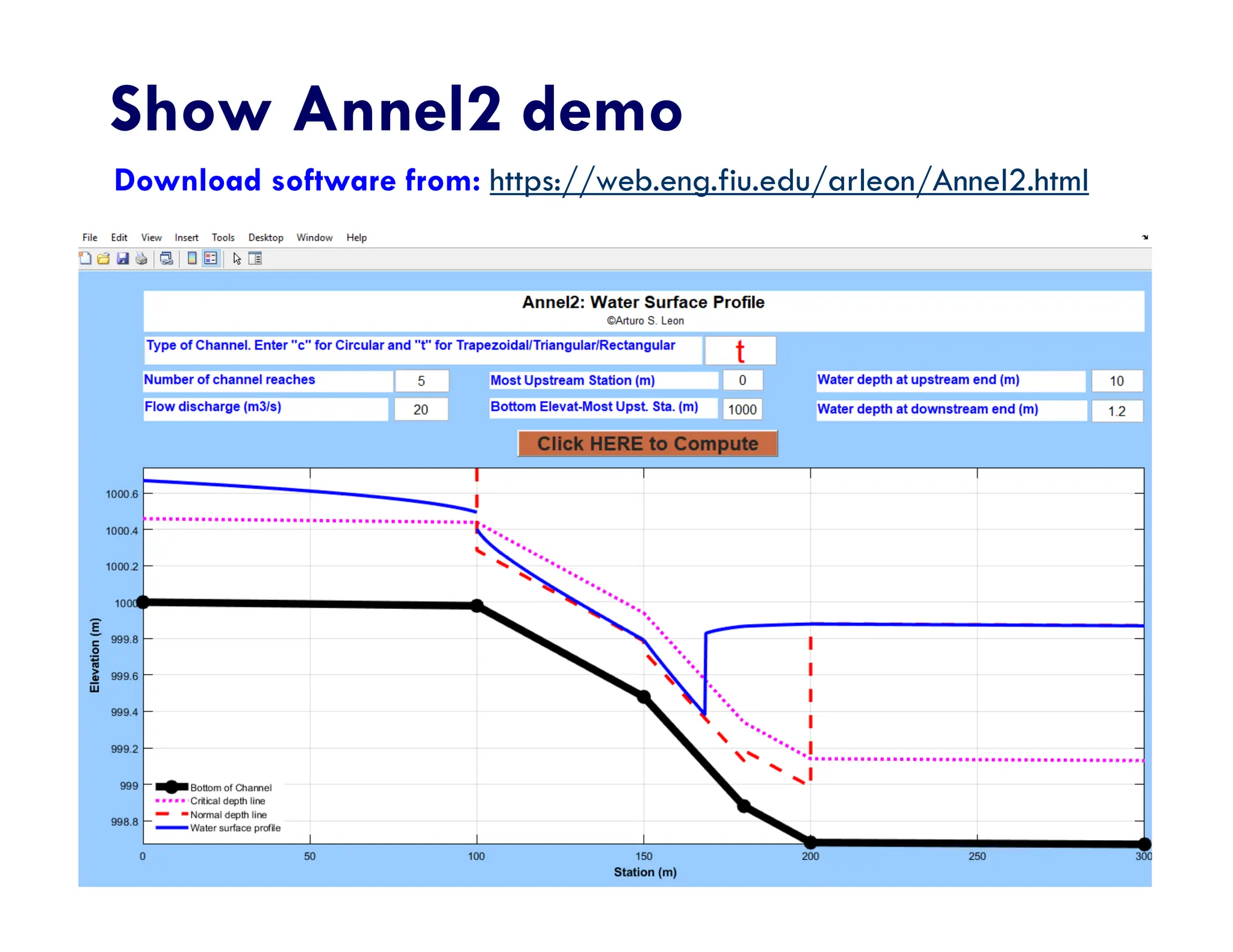
● Several programs are available for modeling mixed
flow regimes
– Annel2 (Arturo Leon)
– HEC-RAS (USACE)
– WSPRO (USGS)

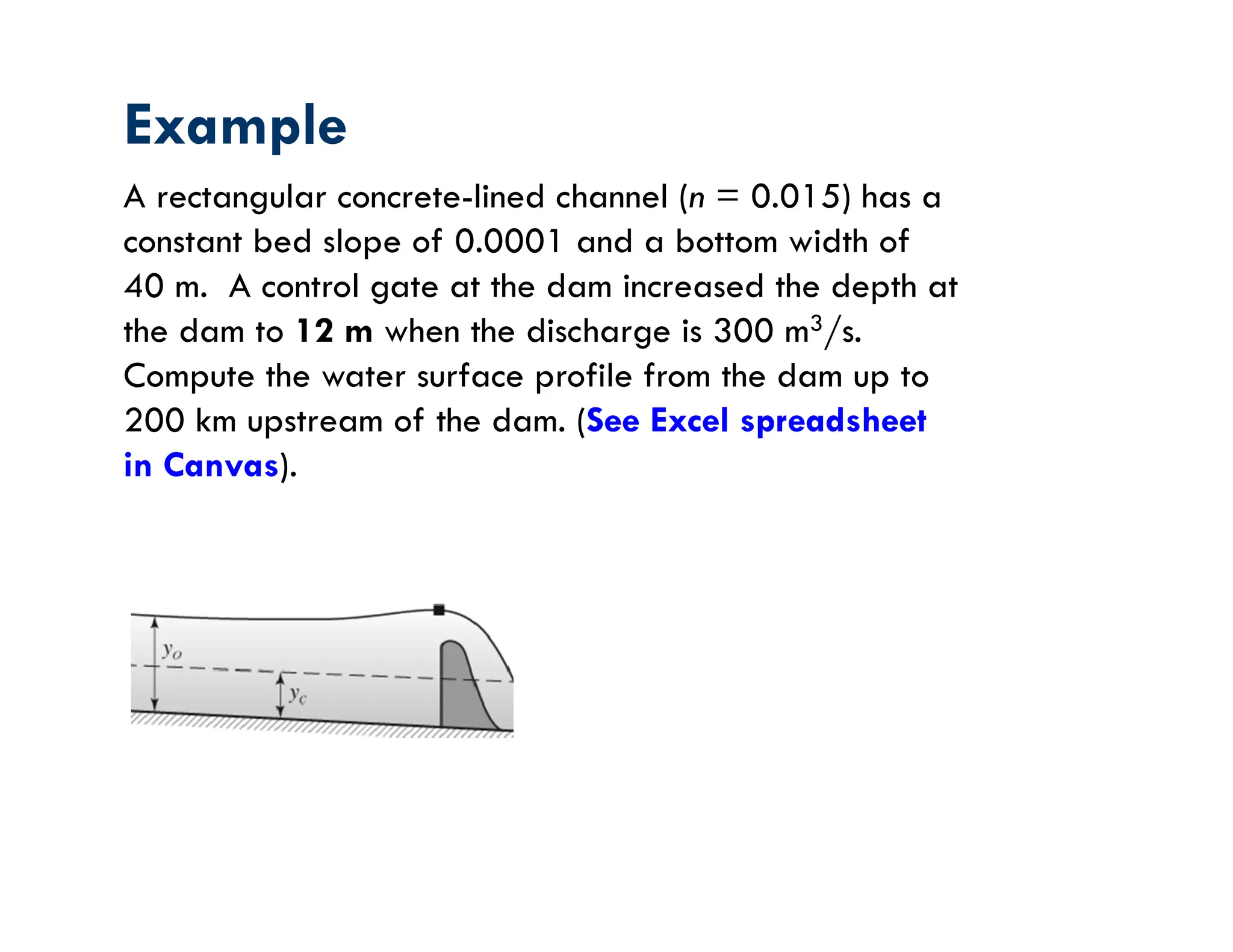
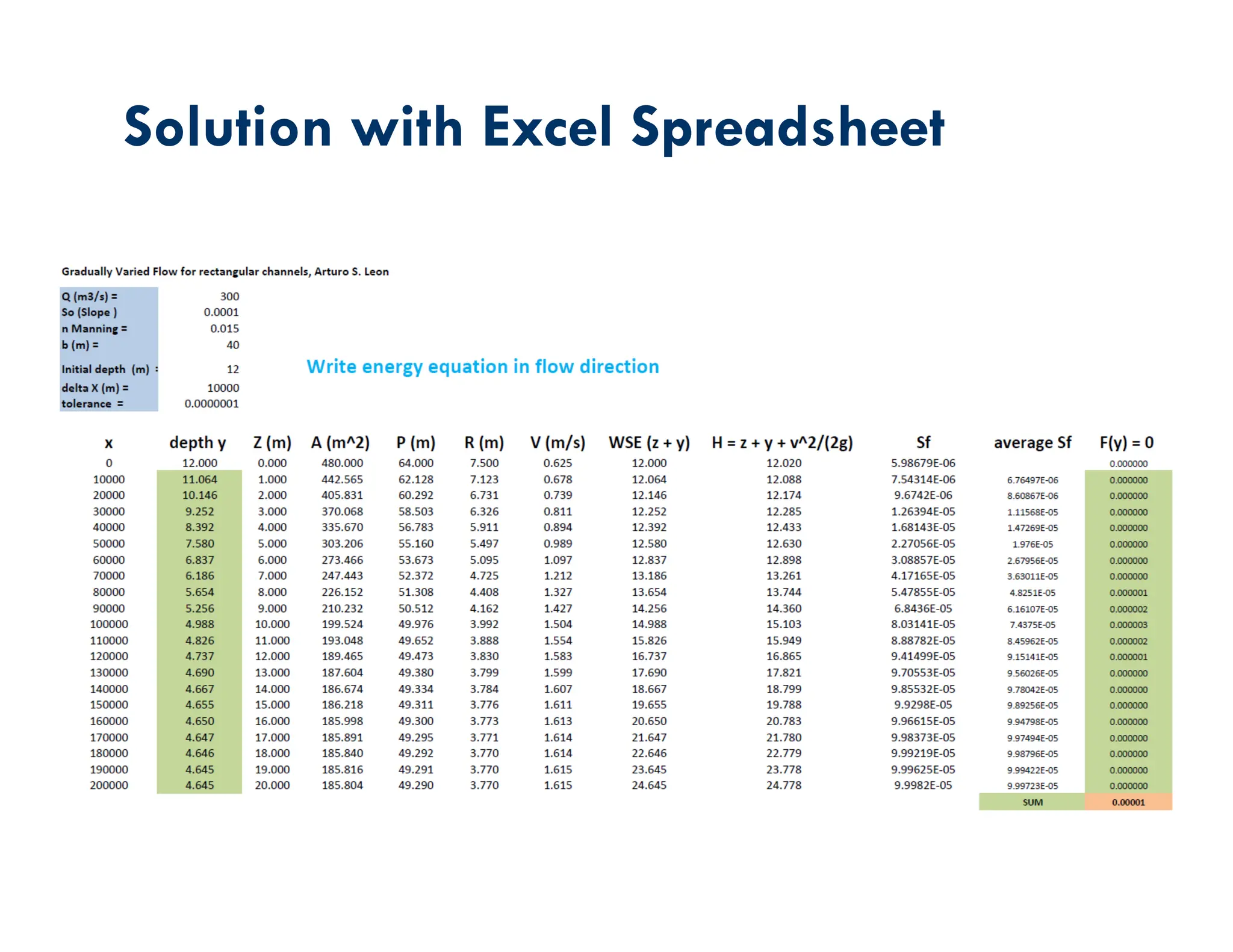
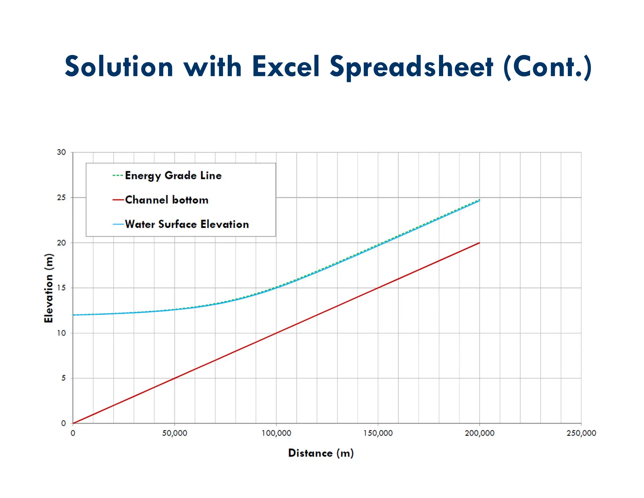
29. Example
A rectangular concrete-lined channel (n = 0.015) has a
constant bed slope of 0.0001 and a bottom width of
40 m. A control gate at the dam increased the depth at
the dam to 12 m when the discharge is 300 m3/s.
Compute the water surface profile from the dam up to
200 km upstream of the dam. (See Excel spreadsheet
in Canvas).

32. Solution with Excel Spreadsheet

33. Solution with Excel Spreadsheet (Cont.)

34. Show Annel2 demo
Download software from: https://web.eng.fiu.edu/arleon/Annel2.html

35. Spatially Varied Flow
(Lateral Weir)

36. Lateral weirs
Source: https://www.youtube.com/watch?v=WayG2RgOwT8
Velocity (m/s)

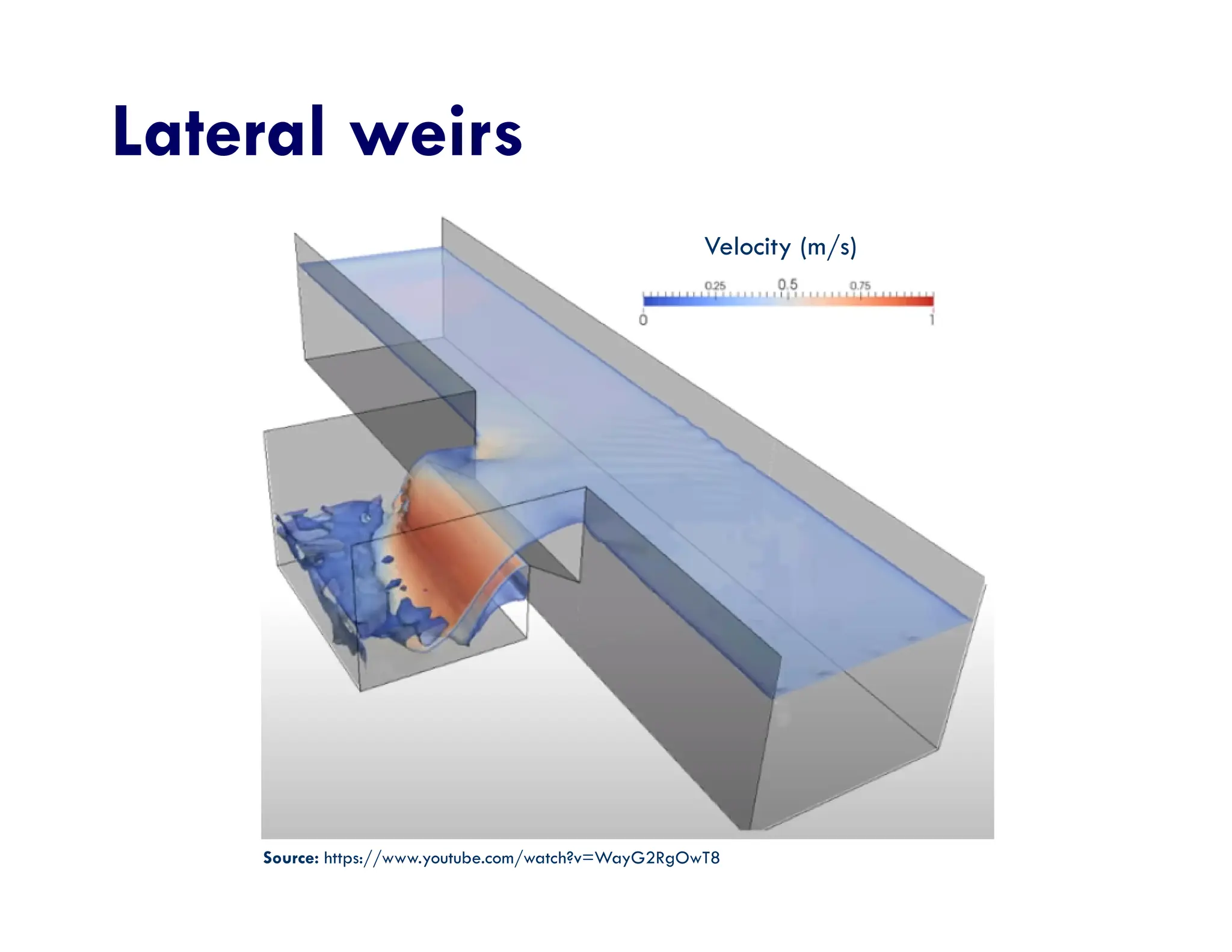
37. Lateral inflow
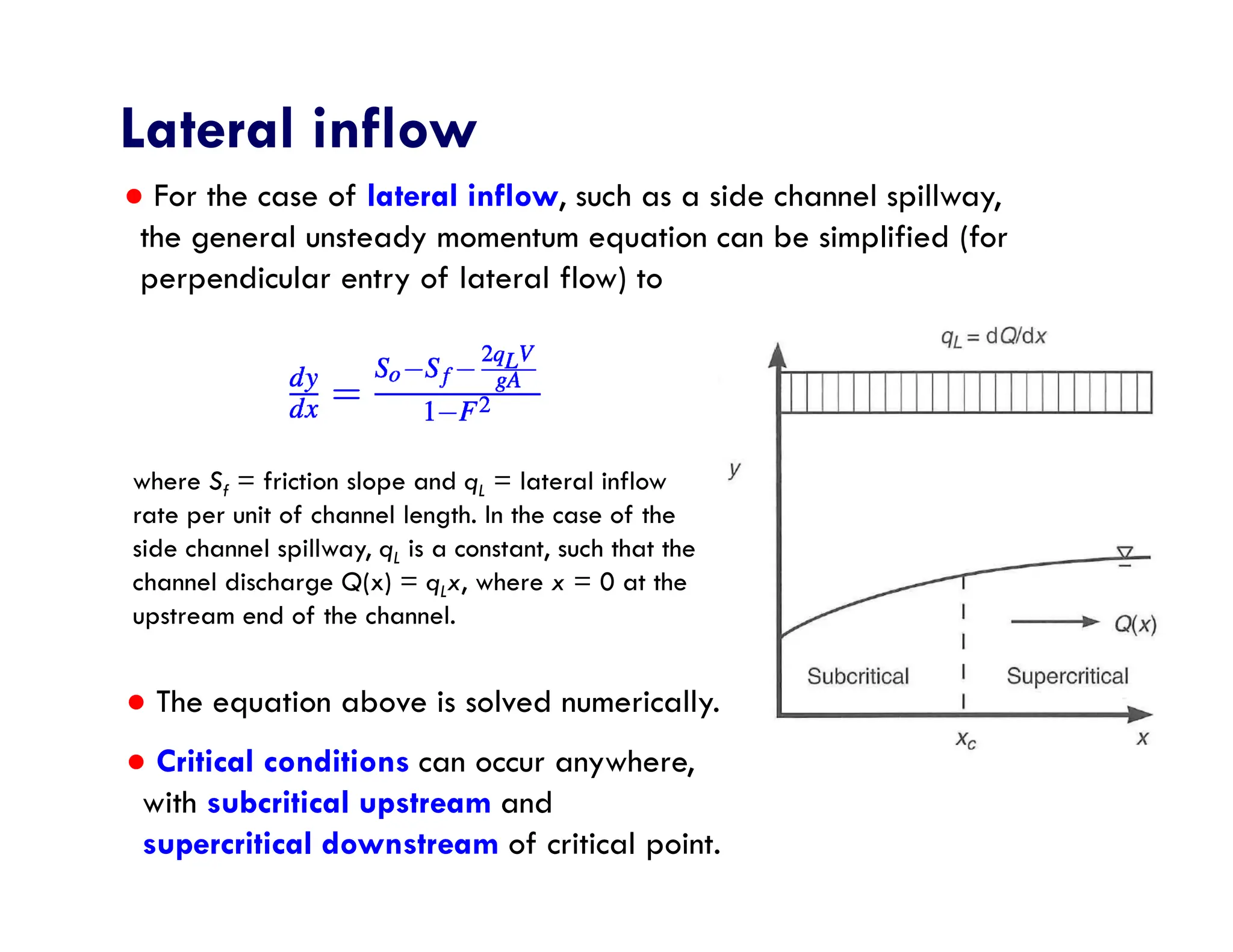
● The equation above is solved numerically.
● Critical conditions can occur anywhere,
with subcritical upstream and
supercritical downstream of critical point.
where Sf = friction slope and qL = lateral inflow
rate per unit of channel length. In the case of the
side channel spillway, qL is a constant, such that the
channel discharge Q(x) = qLx, where x = 0 at the
upstream end of the channel.
● For the case of lateral inflow, such as a side channel spillway,
the general unsteady momentum equation can be simplified (for
perpendicular entry of lateral flow) to

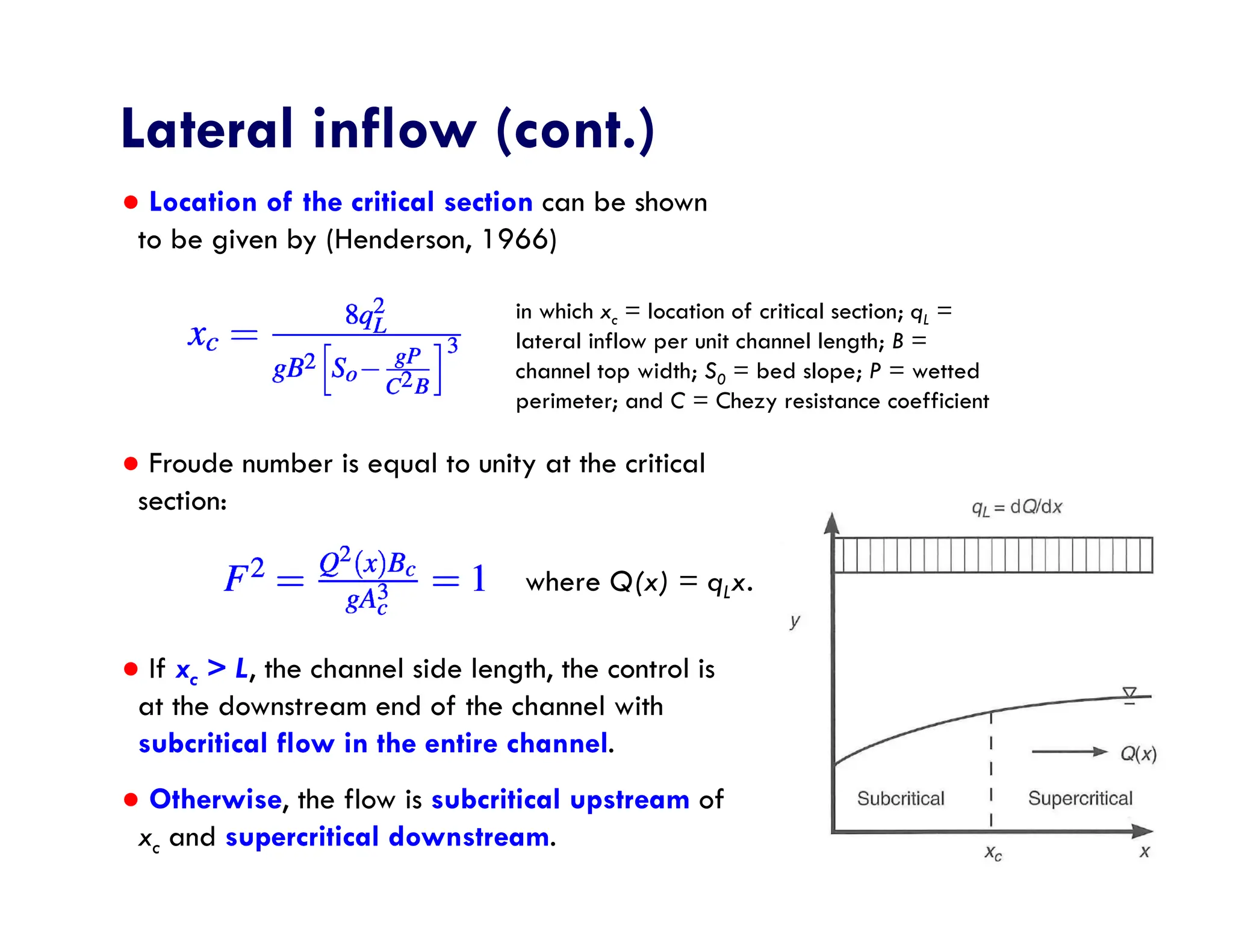
38. ● Location of the critical section can be shown
to be given by (Henderson, 1966)
● Froude number is equal to unity at the critical
section:
● If xc > L, the channel side length, the control is
at the downstream end of the channel with
subcritical flow in the entire channel.
● Otherwise, the flow is subcritical upstream of
xc and supercritical downstream.
Lateral inflow (cont.)
in which xc = location of critical section; qL =
lateral inflow per unit channel length; B =
channel top width; S0 = bed slope; P = wetted
perimeter; and C = Chezy resistance coefficient
where Q(x) = qLx.

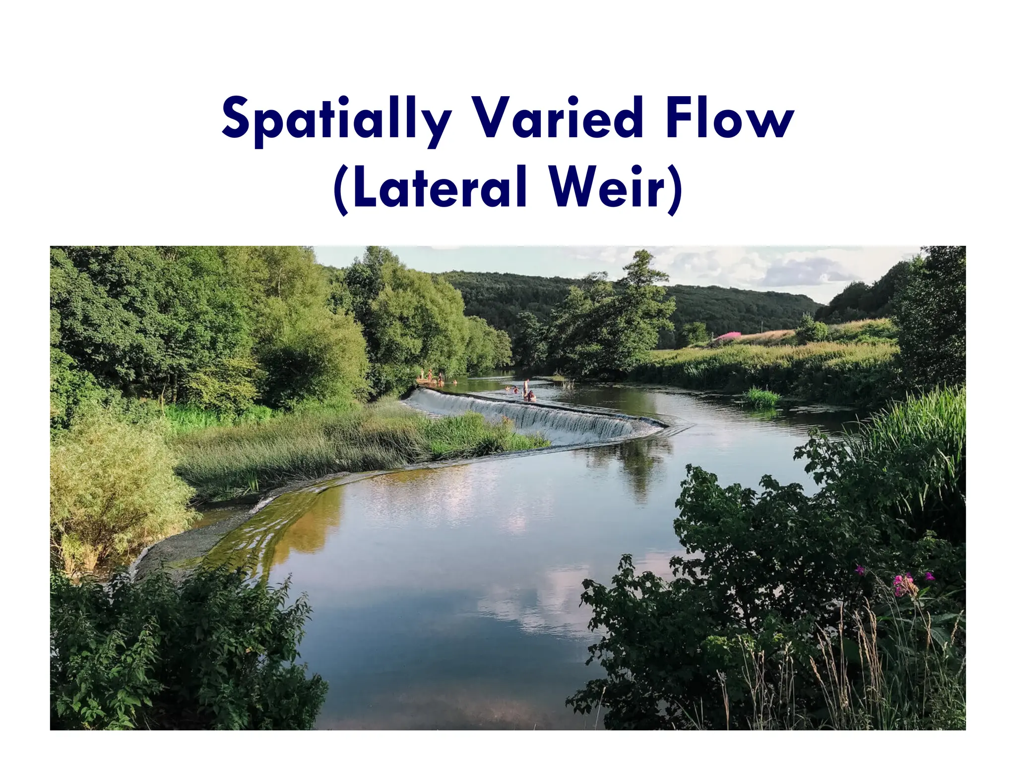
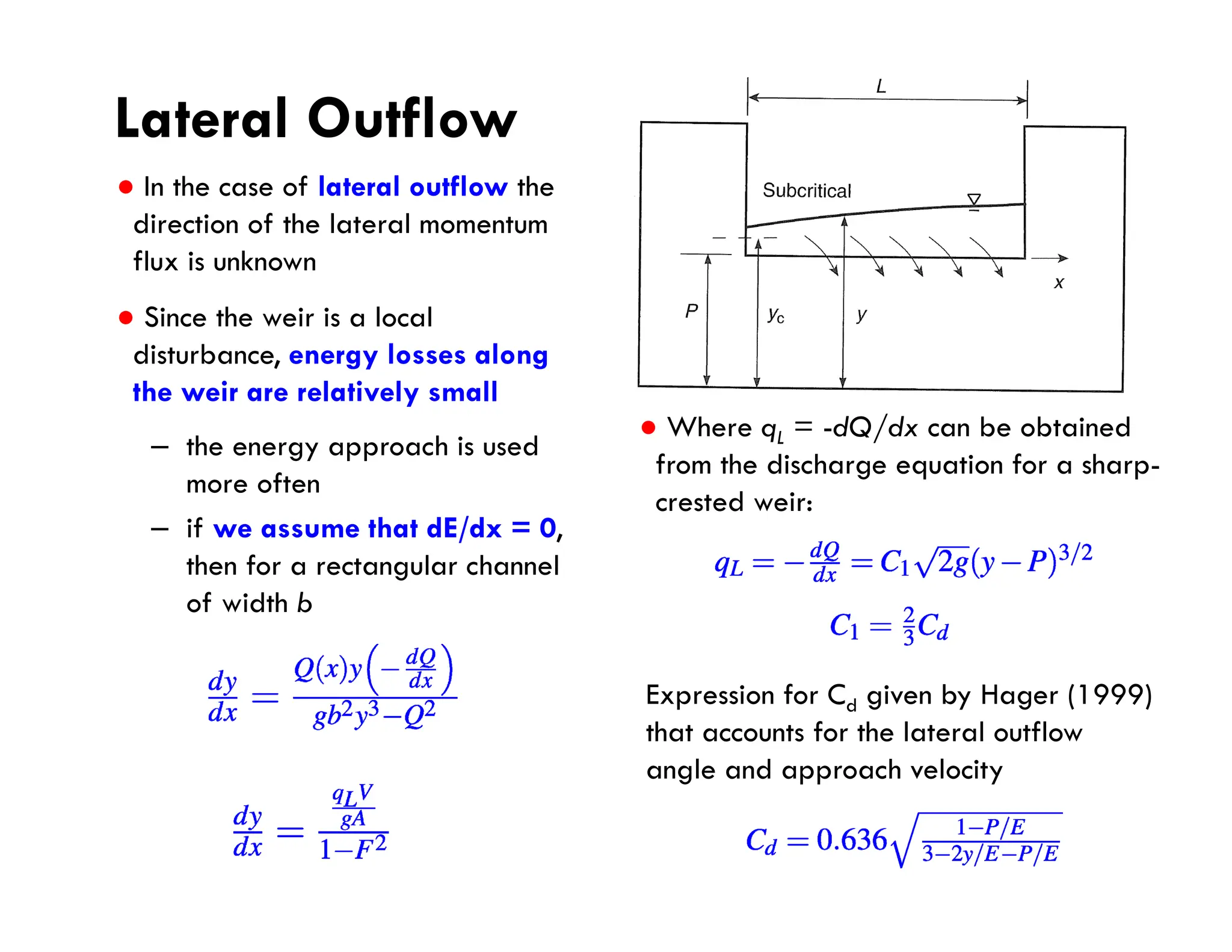
39. Lateral Outflow
● In the case of lateral outflow the
direction of the lateral momentum
flux is unknown
● Since the weir is a local
disturbance, energy losses along
the weir are relatively small
– the energy approach is used
more often
– if we assume that dE/dx = 0,
then for a rectangular channel
of width b
● Where qL = -dQ/dx can be obtained
from the discharge equation for a sharp-
crested weir:
Expression for Cd given by Hager (1999)
that accounts for the lateral outflow
angle and approach velocity

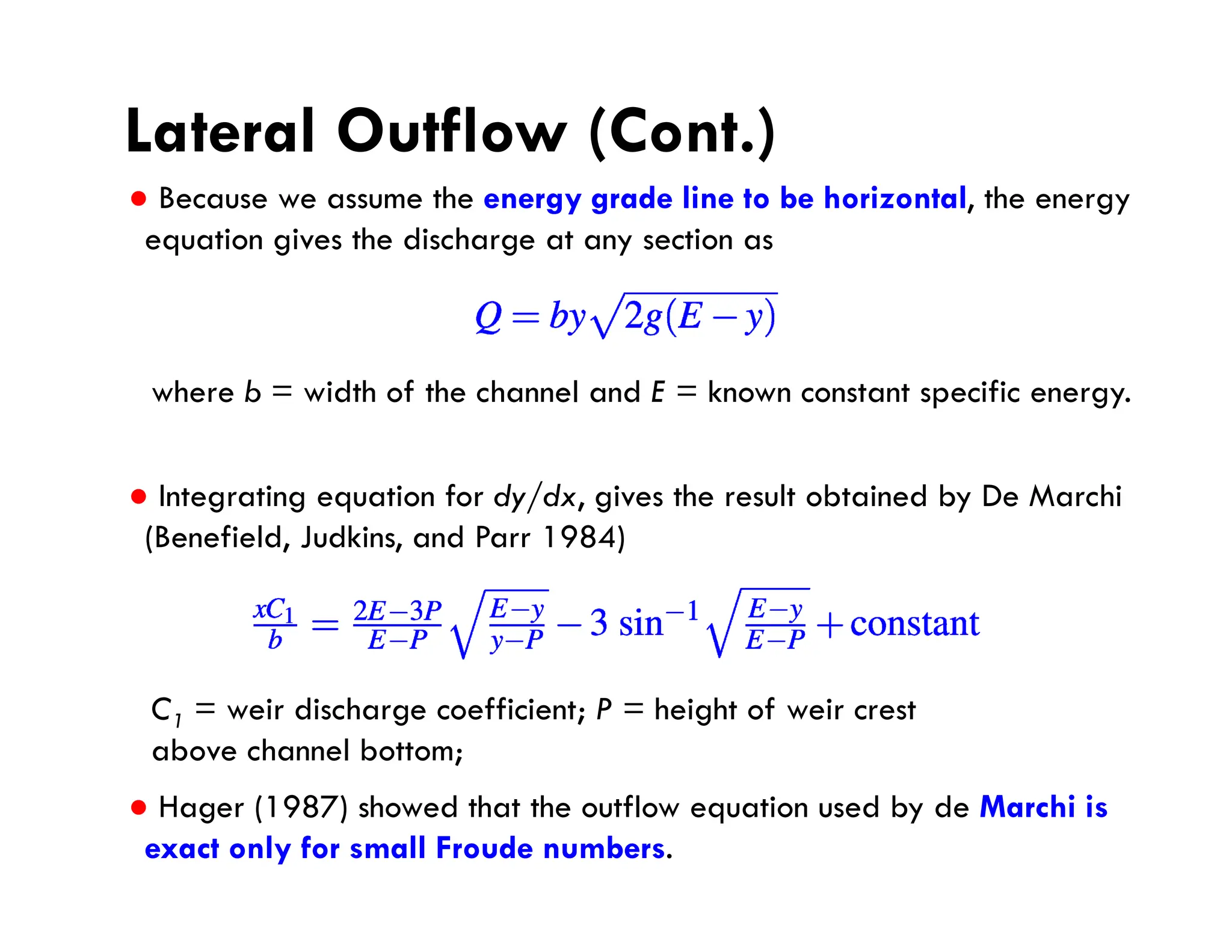
40. Lateral Outflow (Cont.)
● Because we assume the energy grade line to be horizontal, the energy
equation gives the discharge at any section as
● Integrating equation for dy/dx, gives the result obtained by De Marchi
(Benefield, Judkins, and Parr 1984)
● Hager (1987) showed that the outflow equation used by de Marchi is
exact only for small Froude numbers.
where b = width of the channel and E = known constant specific energy.
C1 = weir discharge coefficient; P = height of weir crest
above channel bottom;

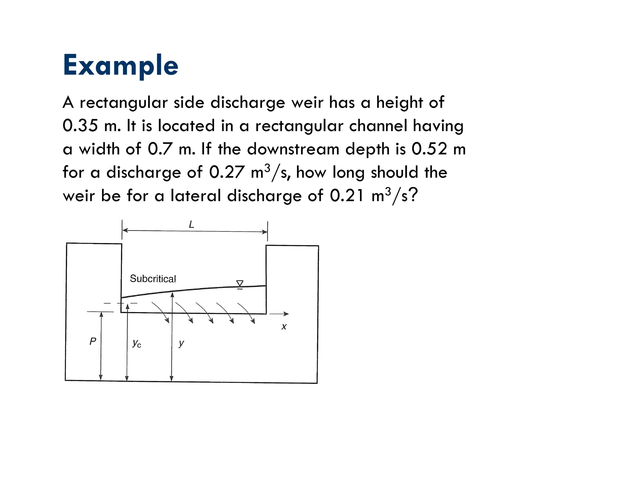
41. Example
A rectangular side discharge weir has a height of
0.35 m. It is located in a rectangular channel having
a width of 0.7 m. If the downstream depth is 0.52 m
for a discharge of 0.27 m3/s, how long should the
weir be for a lateral discharge of 0.21 m3/s?